Article

Predicting Discharge Coefficient of Triangular Side Orifice Using LSSVM Optimized by Gravity Search Algorithm

by
Payam Khosravinia
1,
Mohammad Reza Nikpour
2,*,
Ozgur Kisi
3,4 and
Rana Muhammad Adnan
5,*
1
Water Sciences and Engineering Department, Faculty of Agriculture, University of Kurdistan, Sanandaj 66177-15175, Iran
2
Water Engineering Department, Faculty of Agriculture and Natural Resources, University of Mohaghegh Ardabili, Ardabil 56199-11367, Iran
3
Department of Civil Engineering, Lübeck University of Applied Sciences, 23562 Lübeck, Germany
4
Civil Engineering Department, Ilia State University, 0162 Tbilisi, Georgia
5
School of Economics and Statistics, Guangzhou University, Guangzhou 510006, China
*
Authors to whom correspondence should be addressed.
Water 2023, 15(7), 1341; https://doi.org/10.3390/w15071341
Submission received: 6 March 2023 / Revised: 22 March 2023 / Accepted: 27 March 2023 / Published: 29 March 2023

Abstract

:
Side orifices are commonly installed in the side of a main channel to spill or divert some of the flow from the source channel to lateral channels. The aim of the present study is the accurate estimation of the discharge coefficient for flow through triangular (Δ-shaped) side orifices by applying three data-driven models including support vector machine (SVM), least squares support vector machine (LSSVM) and least squares support vector machine improved by gravity search algorithm (LSSVM-GSA). The discharge coefficient was estimated by utilizing five dimensionless variables resulted from experimental data (570 runs). Five different scenarios were applied based on the input variables. The models were evaluated through several statistical indices and graphical charts. The results showed that all of the models could successfully estimate the discharge coefficient of Δ-shaped side orifices with adequate accuracy. However, the LSSVM-GSA produced the best performance for the input combination of all variables with the highest coefficients of determination (R2) and Nash–Sutcliffe efficiency (NSE), equal to 0.965 and 0.993, and the least root mean square error (RMSE) and mean absolute error (MAE), equal to 0.0099 and 0.0077, respectively. The LSSVM-GSA improved the RMSE of the SVM and LSSVM by 26% and 20% in estimating the discharge coefficient. Furthermore, the ratio of orifice crest height to orifice height (W/H) was identified as having the highest influence on the discharge coefficient of triangular side orifices among the various input variables.

1. Introduction

Side orifices, sluice gates and side weirs are diverting structures in open channels and they are used for diverting some of the main channel flow to side channels and regulating the head of distributaries. In addition, they are commonly utilized in wastewater treatment systems, irrigation and drainage networks, sedimentation tanks and aeration basins [1,2]. Accurate estimation of the discharge coefficient is necessary to know the volume of water passing through the diversion structures. To date, many experiment-based and analytical studies have been done to estimate the discharge coefficient in flow diversion structures.
Ramamurthy et al. [3,4] were the first researchers who experimentally studied the hydraulic properties of rectangular side orifices. They provided equations for computing the orifice discharge coefficient based on the parameters of orifice length, main channel width and ratio of the main channel velocity to the orifice jet velocity. Gill [5] proposed equations for predicting the discharge of circular and rectangular side orifices in the closed conduit flow (in both gravity and pressurized flows) by analytically solving the steady varied flow. Hussain et al. [1] performed experiments under free-flow conditions to provide regression equations for computing the discharge coefficient of rectangular side orifices in small and large sizes, based on the Froude number and the ratio of orifice width to channel width. Hussain et al. [6] obtained an equation to calculate the discharge through rectangular side orifices using analytical relationships with ±5% accuracy. Hussain et al. [7,8] performed experimental and analytical studies to examine the hydraulic properties of flow in sharp-crested circular side orifices and presented equations to compute the discharge coefficient of circular side orifices based on the ratio of the orifice diameter to the main channel width and flow Froude number, under free- and submerged-flow conditions. Bryant et al. [9] and Guo and Stitt [10] investigated the flow of circular orifices for different hydraulic conditions by applying physical and analytical models and derived analytical relationships for the discharge calculation. Vatankhah and Mirnia [
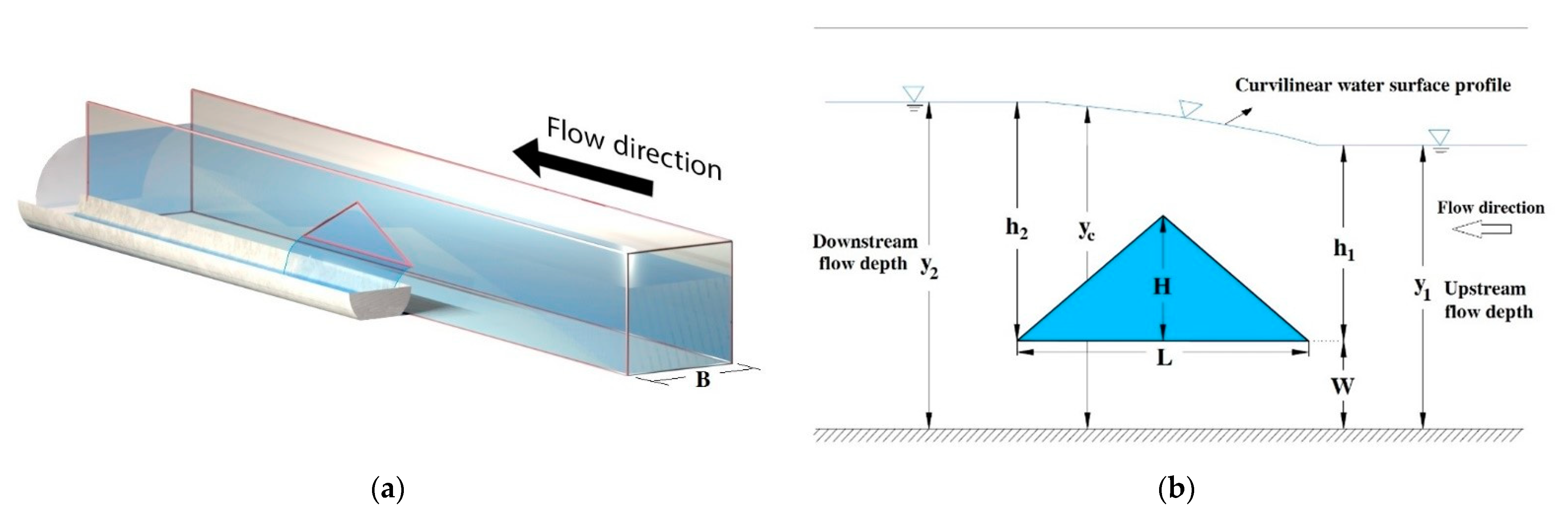
2], for the first time, experimentally and analytically investigated the flow through a sharp-crested side triangular orifice (Δ-shaped orifice) located in a rectangular channel and presented equations for computing the discharge coefficient.
In order to estimate the discharge coefficient of side weirs, another diversion structure in open channels, experimental studies have been performed for rectangular [11,12,13,14] and triangular sections [15,16,17] in subcritical conditions.
Currently, applying soft computing has been accepted as an efficient tool for mapping the complex and nonlinear systems and has been commonly utilized in the water sciences to predict various hydraulic and hydrological parameters. Various data-intelligent techniques including neuro-fuzzy (ANFIS), gene expression programming (GEP), multi-layer perceptron (MLP), extreme learning machine (ELM), group method data handling (GMDH) and support vector machine (SVM) have been utilized for predicting the discharge coefficient of rectangular side weirs [18,19,20,21,22,23,24,25,26,27]. Granata et al. [28] developed two lazy machine learning algorithms, k-Nearest Neighbor and K-Star, for predicting the Cd of a side weir in a circular channel under a supercritical flow regime. Both of the algorithms outperformed the empirical equations of Biggiero et al. and Hager. Li et al. [29] provided the machine learning models ANN, SVM and extreme learning machine (ELM) for the prediction of the discharges of rectangular sharp-crested weirs. They found that all three models were capable of predicting the Cd with high accuracy, but the SVM exhibited somewhat better performance.
The discharge coefficient of triangular labyrinth side weirs has also been successfully predicted using intelligent models [30,31,32,33,34,35,36,37]. Dutta et al. [38] carried out experiments in a rectangular flume under free-flow to investigate the discharge capacity of a multi-cycle W-form labyrinth weir and a sharp-crested circular arc weir. They utilized the experimental data for building predictive models using multiple linear regression (MLR), SVM and ANN. They observed that the SVM model performed better than the rest of the models in predicting the discharge.
A few studies have been conducted to predict the discharge coefficient of circular and rectangular side orifices using data-driven techniques [39,40,41]. Roushangar et al. [42] evaluated the potential of two different machine learning methods, namely support vector machines combined with genetic algorithm (SVM–GA) and GEP, for predicting the Cd of trapezoidal and rectangular sharp-crested side weirs. The results showed that the SVM–GA model gave more accurate outputs than the GEP.
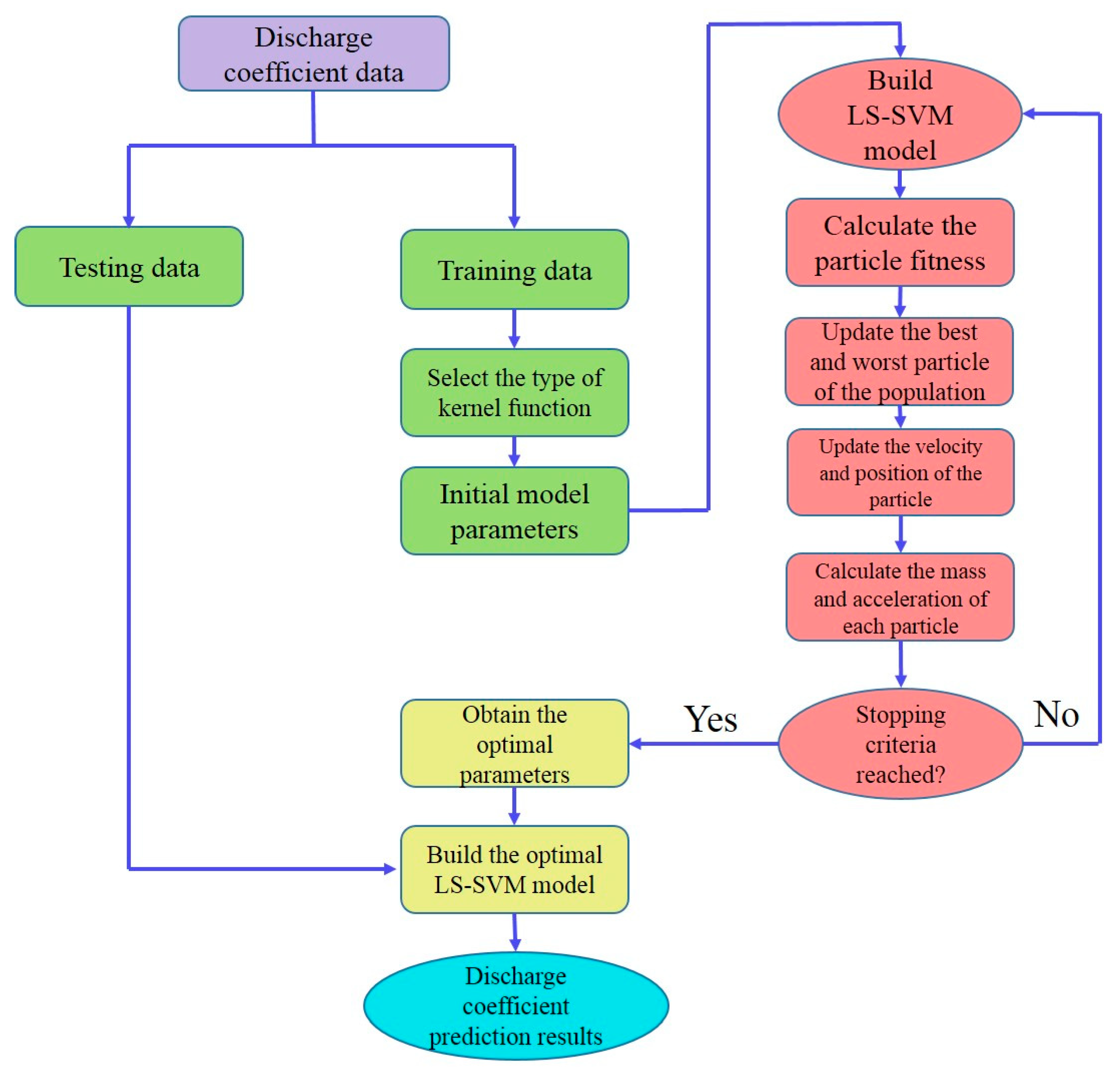
Due to the importance of accurately determining the discharge of side orifices in open channels, in the presented work, for the first time, new and efficient data-driven models including SVM, least squares support vector machine (LSSVM) and LSSVM with gravity search algorithm (LSSVM-GSA) were applied for modeling the discharge coefficient of triangular (Δ-shaped) side orifices. For this purpose, laboratory data of Vatankhah and Mirnia [2] were used. It should be noted that there are a few studies on the application of GSA in the water resources field such as a hybrid model of an artificial neural network with GSA (ANN–GSA) in rainfall-runoff modeling [43], an LSSVM-GSA hybrid model in the prediction of wind power [44,45], an MLP-GSA hybrid model in the prediction of lake water surface [46], a GSA in water tank optimization [47] and an LSSVM–GSA in river flow forecasting [48].

2. Materials and Methods

2.1. Discharge Equation of Triangular Side Orifice

Figure 1 demonstrates water surface profile in an equilateral Δ–shaped side orifice with the height of H and length of L, located in a horizontal rectangular channel under subcritical regime. In this Figure, h1 and h2 represent elevation of water from the free surface to the orifice crest at the upstream and downstream ends of the orifice. In addition, the flow depths at upstream and downstream ends of the orifice are shown by y1 and y2 [2].
As can be observed, curvilinear water surface profile increases from upstream to downstream along the side orifice. Based on the analytical consideration, the below equation is used for obtaining the discharge through a triangular side orifice [2]:
Q = C d L H 2 2 g h c
where hc is the flow height above the centroid of orifice section that is calculated from:
h c = y c W H / 3
where yc denotes flow depth from the surface of the water to the bed channel at above side orifice (see Figure 1).

2.2. Analyzing Discharge Coefficient of a Triangular Side Orifice

There are different hydraulic and geometric parameters that affect the discharge coefficient of Δ-shaped side orifices (Cd). These parameters include height (H) and length (L) of the orifice, crest height of the orifice (W), upstream flow depth in the main channel (y1), upstream velocity in the main channel (V1), width of the main channel (B), water density (ρ), water viscosity (μ), acceleration due to gravity (g) and water surface tension (σ). Hence, the following function can be used for expressing the discharge coefficient of triangular side orifices:
C d = F 1 ( L , H , W , B , y 1 , V 1 , g , σ , μ , ρ )
The respective functional relationship can be expressed as follows using Buckingham’s theory, where the dimensionless parameters with non-significant effects have been neglected:
C d = F 2 ( W H , B L , B H ,   y 1 H , F r 1 = V 1 g y 1 )
where Fr1 represents the Froude number.
In the current research, we investigate the impact of dimensionless parameters of Equation (4) on the discharge coefficient of the triangular side orifice using data-driven models.

2.3. Experimental Data

In the present work, the experimental data of triangular side orifices provided by Vatankhah and Mirnia [2] were utilized for developing the models in the training and validation stages. A set of 570 laboratory data is utilized in this work, consisting of 12 geometric configurations (i.e., two different lengths of orifice (L), three different heights of orifice (H) and two different crest heights (W)). For the application of data-driven models, the available laboratory data set is divided into training and testing parts. A set of 400 data points out of 570 is used as training dataset (70%), whereas remaining 170 data points are used as testing dataset (30%). The measured data range used in the present study have been given in Table 1.
According to this table, discharge values of the main channel (Qu) and side orifice (Qs) are in the range of 13.33–34.64 (L/s) and 1.7–17.6 (L/s), respectively. Moreover, the changes of the Froude number imply that all the experiments have been performed under free-flow conditions.

2.4. Support Vector Machine (SVM)

SVM is a regression and classification approach derived from statistical learning theory [49]. The SVM classification technique is one of the basic approaches used in machine learning and based on structural risk minimization.
This learning system is utilized to cluster and measure the data-fitting function. Estimation of the relationship of the dependent variable (y) on a set of independent variables (x) is required for the SVM regression model. Moreover, similar to other regression problems, it is presumed that the relationship between independent and dependent variables is given by the function f(x) with some noise [49]:
y = f ( x ) + n o i s e = [ w . ( x ) + b ] + c
where w represents vector of coefficients, ϕ(x) is the kernel function and ε and b represent bias term and the regression equation error. Thus, the ultimate goal is finding an appropriate form of the function f(x) that can present the proper training of the SVM model by the use of the training data aimed at minimization of the error function. The following optimization problem is presented [50]:
min   1 2 | | w | | 2 + C c i = 1 n ( ξ i + ξ i )
y i b [ w . ϕ ( X i ) ] ε + ξ i
Subject   to   [ w . ϕ ( X i ) ] + b y i ε + ξ i ξ i . ξ i
where yi represents the measured value by the model, Cc denotes the capacity parameter and ξ i and ξ i represent the Slack variables. The kernel functions are used in SVM model for solving nonlinear problems. There are different kernel functions in SVM model, including sigmoid kernel, Gaussian radial base kernel function (RBF) and polynomial kernel [44]. The equations of common kernel functions [51] have been given in Table 2. In the present research, among various kernel functions, the radial basis function (RBF) was utilized to model the Cd of Δ-shaped side orifices, because the superiority of this kernel over the other two alternatives is proved by the existing literature.

2.5. Least Squares Support Vector Machines (LSSVM)

Dual programming is utilized in SVM model for solving the equations. Hence, there is a large computational cost to solve large-scale problems using this model. Suykens and Vandewalle [52] solved this problem and presented the least squares of support vector machine (LSSVM) approach. Simple linear equations are used in this model for solving the problems, which decreases the algorithm complexity [53]. LSSVM algorithm process has been shown in Figure 2.
The following nonlinear regression function is employed in this model for estimating the problems [54]:
y ( x ) = w T ϕ ( x ) + b
The regular function should be minimized in order to estimate function in LSSVM approach, which is formulated as follows [54]:
m i n R ( w , e ) = 1 2 W T w + γ 2 i = 1 n e i 2
It is subjected to the following constraints:
y ( x ) = w T ϕ ( x i ) + b + e i i = 1 , 2 , , n
where γ and ei refer to the regularization parameter and error in the training phase. For solving this optimization problem, the Lagrange function is employed for finding the w and e solutions. The Lagrange function is presented below:
L ( w , b , e , α ) = 1 2 W T w + γ 2 i = 1 n e i 2 i = 1 n α i { W T ϕ ( x i ) + b + e i y i }
where ai denotes a Lagrange multiplier. Equation (8) can be solved through calculation of the partial differential of the Lagrange function and application of the kernel function (KF) for satisfying the Mercer’s condition. Equation (11) is solved by partial differential with regard to b, w, ei and ai:
L b = 0 w = i = 1 n α i = 0
L w = 0 w = i = 1 n α i ϕ ( x i )
L e i = 0 α i = γ e i
L α i = 0 w T ϕ   ( x i ) + b + e i y i = 0
After removal of ei and w, it is possible to write the following set of linear equations as below [55]:
[ 0 1 T 1 ϕ ( X i ) T ϕ ( X j ) + γ 1 I ] [ b α ] = [ 0 y ]
where α = [α1, …, αn] and y = [y1, …, yn]. Hence, LSSVM model for estimation of function is given as follows:
y ( x ) = i = 1 n α i K ( x i , x ) + b
where α i and b represent answers for Equation (9). The LSSVM has hyper-parameters combination (γ,σ), where regularization factor γ is controlling the exchange between the model smoothness and accuracy, and the kernel parameter σ is controlling the distance among the training points and the model interpolation smoothness. No specific way is available for calculating the optimal values of the hyper-parameters. Therefore, we adopted GSA in the present research for obtaining the appropriate values of the hyper-parameters.

2.6. The Gravitational Search Algorithm (GSA)

GSA was developed by Rashedi et al. [56] as a heuristic stochastic search method. In the mentioned algorithm, the characteristics of each mass (inertial mass, position, velocity and gravitational mass) are important for finding the solution. The mass position is the solution for the gravitational problem, and inertia masses lead the algorithm to the optimal solution or the best mass position. The masses attract each other and the lighter mass is pulled by the heavier one depending on the Newtonian laws concerning motion and gravity (Figure 3).
Assume a system with n masses and the ith mass position given as [57]:
X i = ( x i 1 , , x i d , x i s ) ,   i = 1 , 2 , , n
where x i d indicates the ith mass position in the dth dimension and s represents the dimension of search space. Each agent’s mass is computed based on its fitness value, as follows:
{ m i ( t ) = f i t i ( t ) w o r s t ( t ) b e s t ( t ) w o r s t ( t ) ,       i = 1 , 2 , , n M i ( t ) = m i ( t ) j = 1 N m j ( t ) ,       0 M i ( t ) < 1
where t denotes time and Mi(t) and fiti(t) are the mass and the fitness value of the ith agent at time t. The best(t) and worst(t) in a minimization problem are expressed as below:
w o r s t ( t ) = m a x j { 1 , n } { f i t j ( t ) } ,   b e s t ( t ) = m i n j { 1 , n } f i t j ( t )
We calculate the total force from a set of heavier masses acting on the mass i in the dimension d at the time t as [57]:
F i d ( t ) = j = 1 ,   j i n r a n d i G ( t ) M j ( t ) × M i ( t ) R i j ( t ) + ε ( x j d ( t ) x i d ( t ) )
where Rij(t) represents the Euclidian distance between the two agents i and j, G(t) denotes the gravitational constant at the time t, ε indicates a small constant and randj denotes a random number between [0, 1].
We used the second Newtonian law of motion for calculating the total gravitational acceleration of ith agent:
a i d ( t ) = F i d ( t ) M i ( t ) = F i d ( t ) = G ( t ) j = 1 ,   j i n r a n d j M j ( t ) R i j ( t ) + ε ( x j d ( t ) x i d ( t ) )
Velocity and position can be updated as:
v i d ( t + 1 ) = r a n d i × v i d ( t ) + a i d
w o r s t ( t ) = m a x j { 1 , n } { f i t j ( t ) } ,   b e s t ( t ) = m i n j { 1 , n } f i t j ( t )
where xi(t + 1) and vi(t + 1) denote the next position and next velocity of the agent and randi represents a uniform random variable in the [0, 1] interval.

2.7. Least Squares Support Vector Machine-Gravitational Search Algorithm (LSSVM–GSA)

We used a combination of GSA and LSSVM approaches for minimizing model error and optimizing the hyper-parameters (γ,σ). This section describes the process of constructing the Cd prediction model using the combination of GSA and LSSVM approaches (LSSVM–GSA), which is also observed in Figure 4.
This process is described below:
(i)
First, all discharge coefficient data sets are divided into parts of training and testing.
(ii)
Then, the proper kernel function and primary parameters for LSSVM–GSA model are selected for making the initial LSSVM model.
(iii)
The particle fitness value is calculated for each agent. In the present work, we selected RMSE as the fitness function.
(iv)
The best-fitted parameter combinations are selected via GSA for obtaining the optimum values for LSSVM parameters.
(v)
In the case that the stopping criterion is not met, the new hybrid of parameters is used for reconstructing the LSSVM. The fitness is computed as long as it fits the stopping criterion.
(vi)
The values of ideal parameters are obtained for building the optimum LSSVM model to forecast discharge coefficient. The testing values are now utilized for the optimum LSSVM for achievement of Cd prediction results.

3. Performance Evaluation Indicators

In this research, root mean square error (RMSE), coefficient of determination (R2), Nash–Sutcliffe efficiency (NSE) and mean absolute error (MAE) were utilized as assessment criteria. The computational relations and the range of these performance metrics have been presented as follows [58]:
R M S E = i = 1 N ( P i O i ) 2 N       [ 0 ,   1 ]
R 2 = ( i = 1 N ( O i O i ¯ ) ( P i P i ¯ ) i = 1 N ( U i U i ¯ ) 2 i = 1 N ( P i P i ¯ ) 2 ) 2       [ 0 , + )
N S E = 1 i = 1 N ( P i O i ) 2 i = 1 N ( O i O i ¯ ) 2       ( , 1 ]
M A E = 1 N I = 1 N | P i O i |       [ 0 , + )
where Pi and Oi are the predicted and observed ith value, respectively. In addition, P i ¯ and O i ¯ are the average of predicted and observed values, respectively.

4. Application of the Models

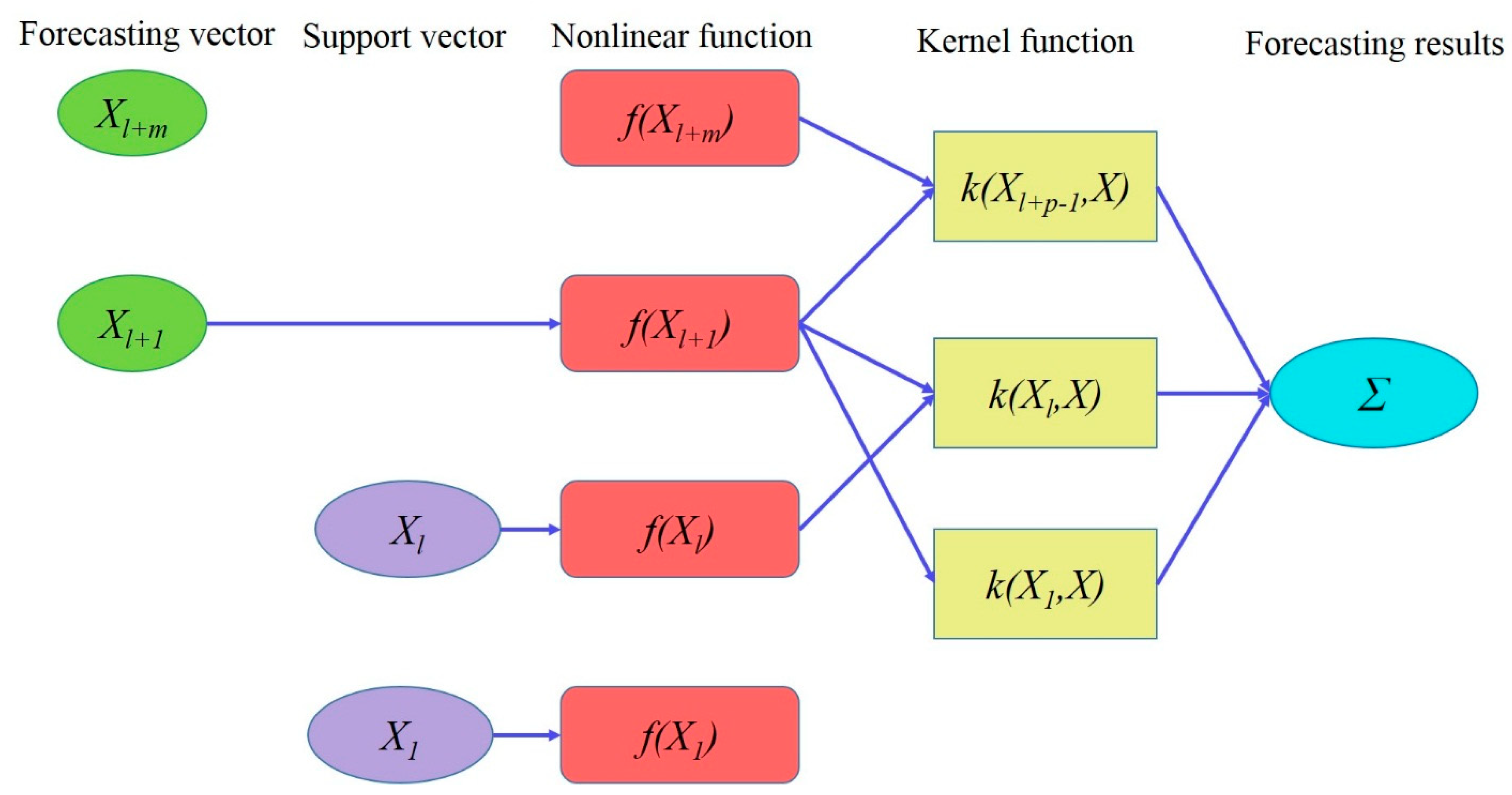
Three data-driven methods, SVM, LSSVM and LSSVM–GSA, were employed for predicting the discharge coefficient of a Δ-shaped side orifice with different hydraulic and geometric conditions.
Table 3 sums up the five different input scenarios considered to predict the discharge coefficient of Δ-shaped side orifices (Cd). Considering the highest correlation (−0.770) between B/H and Cd, this parameter was selected as the first input combination. To compose the other combinations, other parameters were involved in the combination one by one at each step. The fifth combination includes all input parameters.
The analysis results showed that the geometrical parameters of Δ-shaped side orifices including height (H) and length (L) had the highest correlation with Cd; therefore, they were used as input variables in the first and second scenarios. The remaining variables were also ranked based on the correlation coefficients and were applied in the subsequent input scenarios.
In order to calibrate the models, firstly, various kernel functions were utilized to develop the SVM model. Radial basis function (RBF) was found as the optimal kernel function due to its better prediction accuracy. The parameter combinations of SVM (C,γ) and (γ,σ) of LSSVM were obtained via trial and error. For each parameter (regularization factor γ and kernel parameter σ), different numbers from 10−5–105, 10−2–102 and 10−3–103, 10−5–105 were applied following previous literature [59,60,
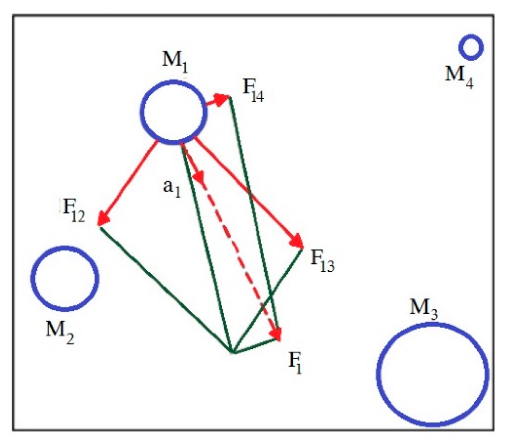
61]. In addition, GSA was employed to get optimized hyper-parameters for the LSSVM. To optimize LSSVM hyper-parameters, control parameter values of the GSA algorithm have a key role, i.e., gravitational constant (G0) and constant alpha (α). Therefore, parameters of LSSVM are found optimal with the G0 parameter in range of 108–114 and α parameter in range of 18–20.
Root mean square error (RMSE) was utilized as the fitness function in the presented work. The optimal hyper-parameters of the LSSVM model obtained by GSA for each input scenario are given in Table 4.

5. Results and Discussion

Table 5 provides the performance metrics of the models used in the current study for the five scenarios defined in Table 3. As can be seen, the performance of the models is similar by considering the applied scenarios. In addition, the models’ error decreased from M1 to M5 by adding the effective variables. Moreover, it is found that by the addition of the W/H variable to the input combination (M4), the accuracy of the models’ results is significantly improved; RMSE decreases from 0.0272 to 0.0156 for SVM, from 0.0227 to 0.0129 for LSSVM and from 0.0217 to 0.0108 for LSSVM-GSA. Additionally, all three methods had the best performance for the M5 input scenario including all five variables (B/H, B/L, Fr1, W/H, H/y1).
The R2, RMSE, MAE and NSE values for the optimal pattern (M5) were obtained as 0.938, 0.0134, 0.0101 and 0.9849 for the SVM model, 0.958, 0.0125, 0.0099 and 0.9895 for the LSSVM model, and 0.965, 0.0099, 0.0077 and 0.9934 for the LSSVM-GSA model, respectively.
It is worth noting that the NSE values of the models utilized in this research were greater than 0.8 for all the models, indicating acceptable accuracy [62,63].
The outcomes reveal that the LSSVM–GSA has superior performance in comparison with other methods for all of the scenarios. In addition, it is clear that the aforementioned model for the M5 pattern with the highest R2 and NSE values and the lowest values of error has the highest power of predicting the Cd of Δ-shaped side orifices. After that, the SVM and LSSVM models rank second and third, respectively. The superiority of the LSSVM–GSA over the SVM and LSSVM has also been seen in the research performed by Yuan et al. [44] and Lu et al. [45].
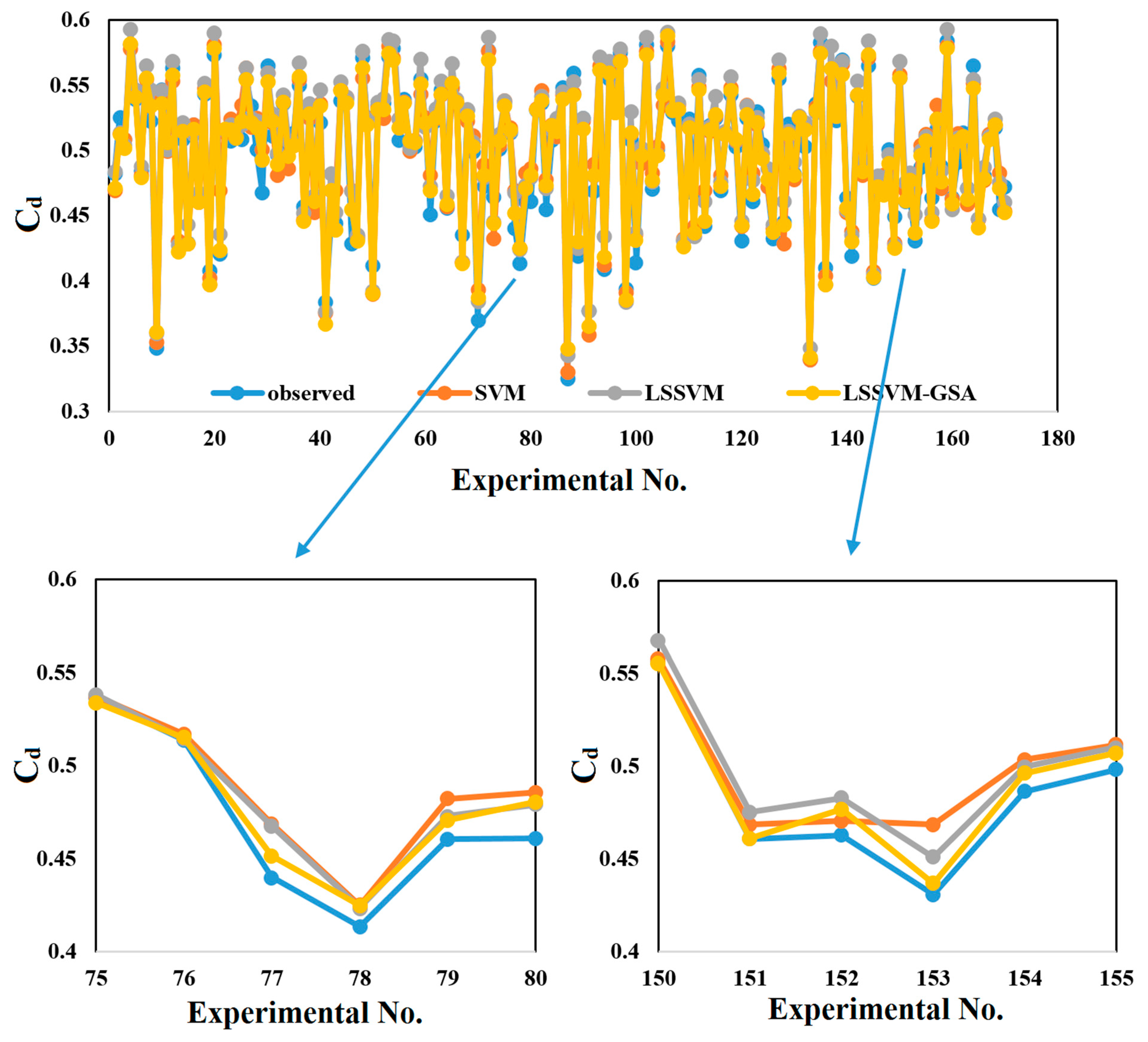
It should be noted that the observed Cd values were in the range of 0.3246–0.5843, while the estimated Cd range for the best responses was 0.3412–0.5872 for the superior model (i.e., LSSVM–GSA).
Figure 5 illustrates the variation graph of observed and predicted Cd values versus experimental No. It is apparent from the detailed parts of the figure (see the two detailed graphs in the lower part of the figure) that the LSSVM–GSA is more successful in catching Cd of Δ-shaped side orifices than the SVM and LSSVM models.
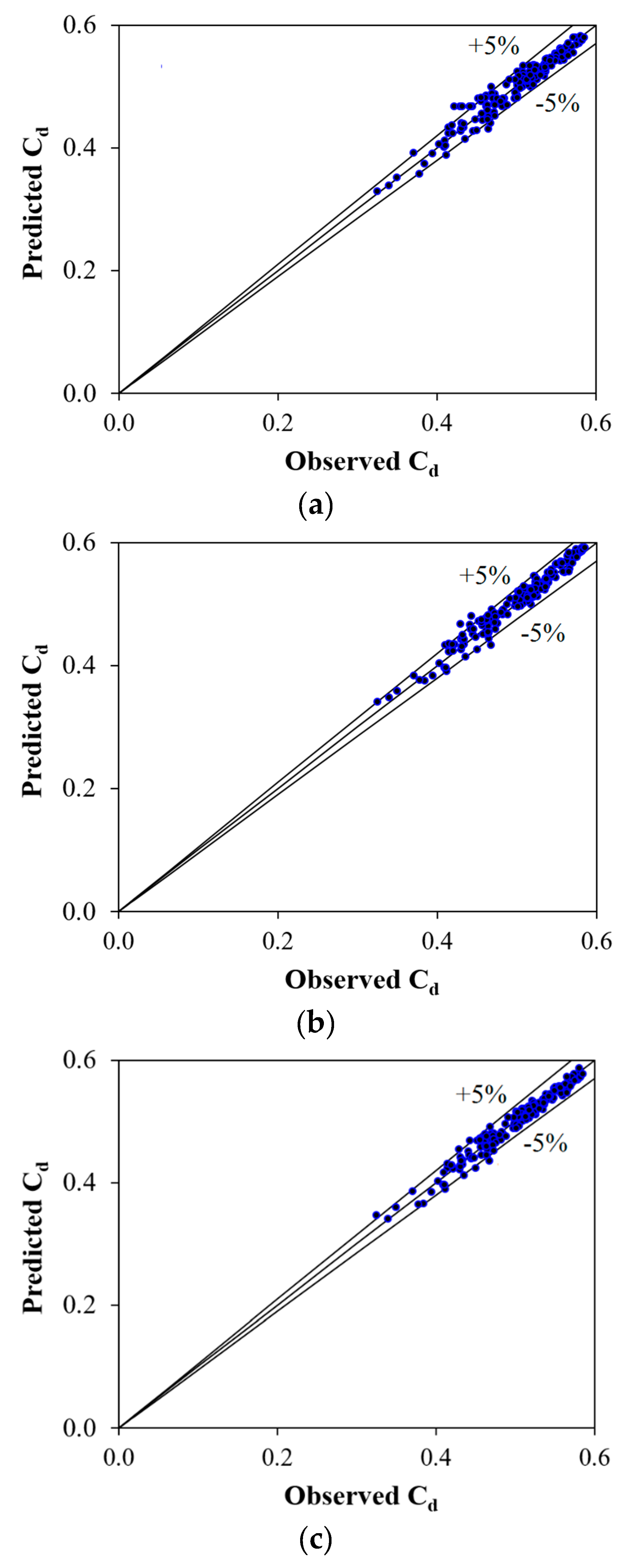
Comparison between the measured and predicted Cd values over the test period for the best input combination (M5) has been depicted in Figure 6. For all the models, very good dispersion is seen around the 45° axis, indicating high capability of the models used in the current work. For 170 discharge data during the test stage for SVM, LSSVM and LSSVM–GSA, 95%, 96% and 97% of the points were situated within the 5% confidence band.
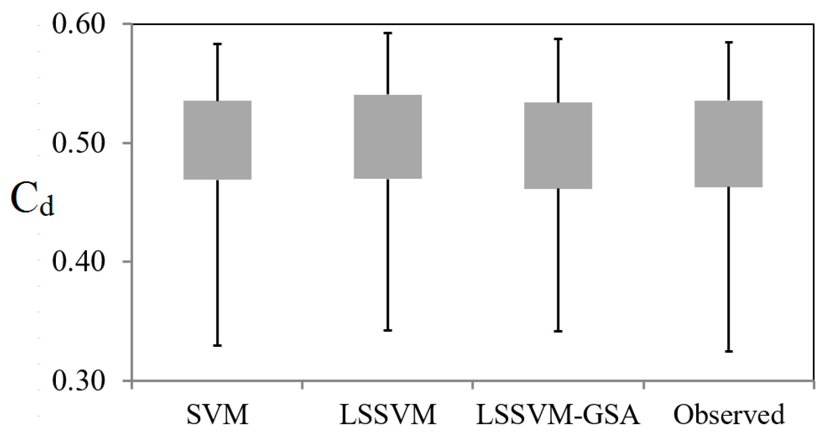
Figure 7 demonstrates a boxplot showing the statistical distribution of the measured and predicted discharge coefficients for the testing period, including the lower quartile, upper quartile and median for the optimal SVM, LSSVM and LSSVM−GSA models. As shown in this plot, for the lower quartile, the SVM model has better yield than the other two approaches. Meanwhile, this range shows the over-prediction of the models. For the median, the LSSVM−GSA model shows complete accordance with the observed values and it is evident that the spread of this model closely resembles the observed Cd values. In addition, the SVM and LSSVM models have some fluctuations in estimating the observed values in the mentioned range. For the upper quartile, the SVM and LSSVM−GSA models have similar accuracy in terms of statistical distribution and matching with the observed values. Additionally, the LSSVM model is found to overestimate the higher Cd values.
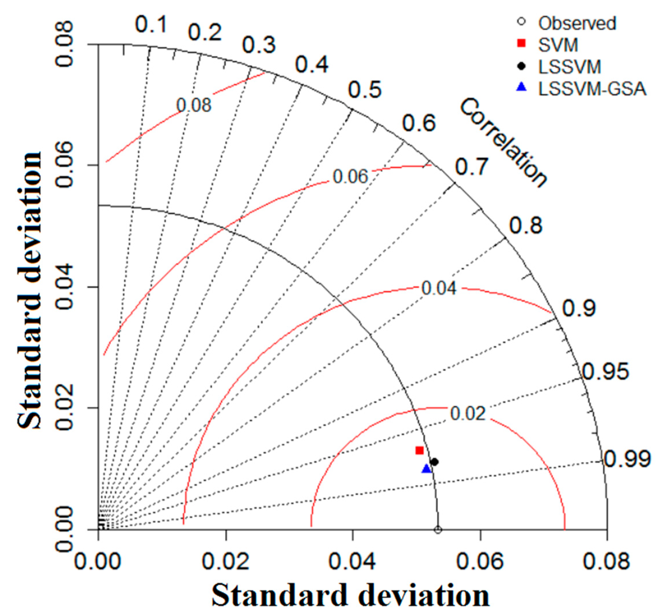
The agreement between the data-intelligent methods and observation values was also checked using another visualization presentation (i.e., Taylor diagram). This graph provides three important statistical indices including centered RMSE, correlation coefficient and standard deviation [64]. Figure 8 displays the Taylor diagram of the predicted and observed values of Cd for the test period and best input combination. As observed in Figure 8, the representative markers of LSSVM and LSSVM−GSA have similar positions; however, the LSSVM−GSA model shows better accuracy than the two other models in terms of RMSE, r and SD indices.
Moreover, run times of the applied models were evaluated. The simulations were done in the MATLAB environment (MATLAB R2017b) using a computer with an operating system of Windows 10 (64 bit) with an Intel(R) Core(TM) i5-10500 CPU @ 3.10 GHz processor with 16 GB RAM. In MATLAB R2017b, LS−SVM lab and Libsvm toolkit were utilized to develop the SVM and LSSVM models, respectively. 
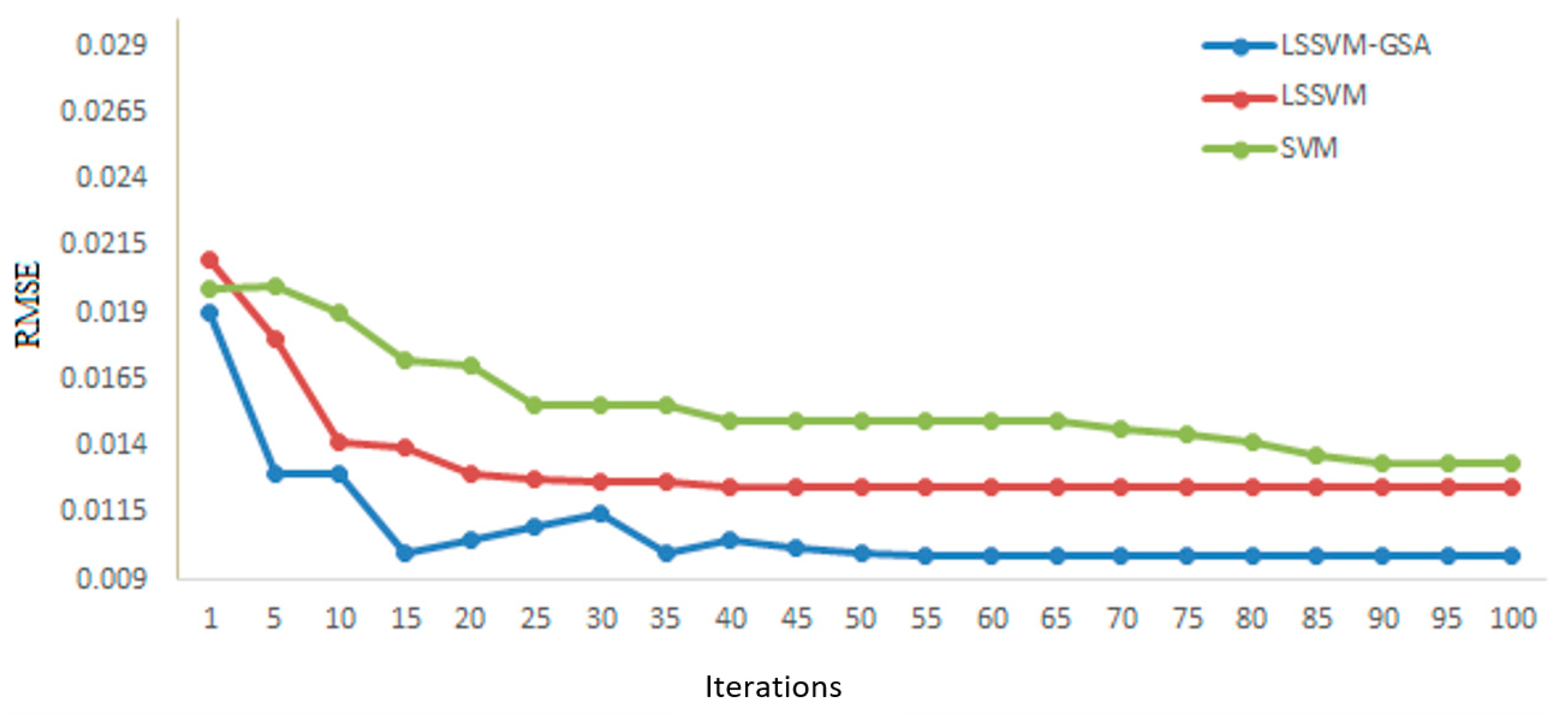
Figure 9 provides the convergence graphs of the implemented models for the best input combination (M5). For the best input scenario, the run times of the SVM, LSSVM and LSSVM−GSA models were 1.534 s, 0.027 s and 26.2 s, respectively. Although the computational cost of the LSSVM-GSA model was higher than the other two models, the aforementioned model had the best prediction accuracy, and moreover, the time required to implement the model is acceptable from an engineering point of view. Similarly, in the research performed by Lu et al. [45], the LSSVM−GSA model was selected as the superior model, with the highest performance and computational time among the implemented models.
The outcomes of the methods were also assessed by one-way analysis of variance (ANOVA) to see the robustness (the possible significant differences between the observations and model predictions) of the methods. The test was set at a significance level of 95%. Table 6 sums up the test results. As observed from the table, the LSSVM−GSA yielded a smaller testing value (0.00004) with a higher significance level (0.995) compared to LSSVM and SVM, and this indicates that the LSSVM−GSA is more robust in predicting the discharge coefficient of triangular side orifices than the other models.

6. Conclusions

Given the importance and wide application of orifices in irrigation and drainage networks, urban water and sewage treatment plants and hydroelectric power facilities, this study was performed to estimate the discharge coefficient of Δ-shaped side orifices. To this end, data-intelligent models including SVM, LSSVM and LSSVM−GSA were applied. Geometric and hydraulic variables were considered as inputs to the models in a set of 570 experimental data. After performing sensitivity analysis, five different input combinations were identified considering the influence of input variables on the output (Cd). According to the statistical indices, the models generally provided satisfactory performance in estimating Cd for all input combinations, and the models had similar sensitivity to the scenario changes and addition of the hydraulic and geometric variables to the input combinations. However, in all of the models, adding the ratio of orifice crest height to orifice height (W/H) into the model input (M4) produced the best accuracy and improvement in RMSE by 42.6%, 43.2% and 50.2% for the SVM, LSSVM and LSSVM−GSA models, respectively. The outcomes also indicated that the LSSVM−GSA improved prediction accuracy over SVM and LSSVM. It was found that optimization of the LSSVM model using the gravity search algorithm (GSA) improved the RMSE by 26% and 20%, respectively, for the best input combination (M5) compared to the SVM and LSSVM models. In addition, based on the visualization inspection (i.e., scatter plots, boxplots and Taylor diagram), the highest correlation and the best statistical distribution of model values belonged to the LSSVM−GSA, although the low discharge coefficients tended to be slightly overestimated when compared to the respective measured values. The overall results of the present study propose the LSSVM optimized with GSA model as a new and efficient model to estimate the discharge coefficient and other hydraulic parameters in open channels.
The present study used a set of 570 experimental data having 12 geometric configurations, and outcomes indicated that the models cannot well catch the low discharge coefficients and this implies that more data is needed to be able to better calibrate the implemented models and obtain better estimation accuracy. The main reason for overestimation of the low values can be related to the convergence criterion (root mean square error (RMSE)). The models focus on catching high values with this criterion. Another criterion (mean absolute error (MAE)) can be tried in future studies to provide a balance in the model estimation accuracy in catching the high and low values. The recommended model (LSSVM−GSA) can also be compared with other improved LSSVM and SVM models with new metaheuristic algorithms and deep learning methods.

Author Contributions

P.K.: Conceptualization, Methodology; M.R.N.: Writing the paper, Original draft preparation; O.K.: Reviewing and editing; R.M.A.: Modeling. All authors have read and agreed to the published version of the manuscript.

Funding

The authors did not receive support from any organization for the submitted work.

Data Availability Statement

Not applicable.

Conflicts of Interest

The authors declare that they have no known competing financial interests or personal relationships that could have appeared to influence the work reported in this paper.

List of Symbols

BThe main channel width (cm)
LLength of the orifice
CdDischarge coefficient
Fr1Upstream Froude number
gGravitational acceleration
HHeight of the triangular side orifice
QsDischarge through the orifice
QuDischarge through the main channel
V1Upstream velocity
WOrifice crest height
y1Upstream flow depth
µWater viscosity
ρThe water density
σwater surface tension
hcflow height above centroid of orifice section
ycflow depth from the surface of the water to the bed channel at above side orifice
yimeasured value by the model
Cccapacity parameter
ξ i , ξ i Slack variables
γregularization parameter
eierror in the train phase
Mi(t)mass value of the ith agent
fiti(t)fitness value of the ith agent
Rij(t)Euclidian distance between the two agents i and j
G(t)gravitational constant
εsmall constant

References

  1. Hussain, A.; Ahmad, Z.; Asawa, G. Flow through sharp-crested rectangular side orifices under free flow condition in open channels. Agric. Water Manag. 2011, 98, 1536–1544. [Google Scholar] [CrossRef]
  2. Vatankhah, A.R.; Mirnia, S.H. Predicting Discharge Coefficient of Triangular Side Orifice under Free Flow Conditions. J. Irrig. Drain. Eng. 2018, 144, 04018030. [Google Scholar] [CrossRef]
  3. Ramamurthy, A.S.; Tim, U.S.; Rao, M.V.J. Weir-Orifice Units for Uniform Flow Distribution. J. Environ. Eng. 1987, 113, 155–166. [Google Scholar] [CrossRef]
  4. Ramamurthy, A.S.; Tim, U.S.; Sarraf, S. Rectangular Lateral Orifices in Open Channels. J. Environ. Eng. 1986, 112, 292–300. [Google Scholar] [CrossRef]
  5. Gill, M.A. Flow through Side Slots. J. Environ. Eng. 1987, 113, 1047–1057. [Google Scholar] [CrossRef]
  6. Hussain, A.; Ahmad, Z.; Ojha, C. Analysis of flow through lateral rectangular orifices in open channels. Flow Meas. Instrum. 2014, 36, 32–35. [Google Scholar] [CrossRef]
  7. Hussain, A.; Ahmad, Z.; Asawa, G. Discharge characteristics of sharp-crested circular side orifices in open channels. Flow Meas. Instrum. 2010, 21, 418–424. [Google Scholar] [CrossRef]
  8. Hussain, A.; Ahmad, Z.; Ojha, C. Flow through lateral circular orifice under free and submerged flow conditions. Flow Meas. Instrum. 2016, 52, 57–66. [Google Scholar] [CrossRef]
  9. Bryant, D.B.; Khan, A.A.; Aziz, N.M. Investigation of Flow Upstream of Orifices. J. Hydraul. Eng. 2008, 134, 98–104. [Google Scholar] [CrossRef]
  10. Guo, J.C.Y.; Stitt, R.P. Flow through Partially Submerged Orifice. J. Irrig. Drain. Eng. 2017, 143, 06017006. [Google Scholar] [CrossRef]
  11. Cheong, H. Discharge Coefficient of Lateral Diversion from Trapezoidal Channel. J. Irrig. Drain. Eng. 1991, 117, 461–475. [Google Scholar] [CrossRef]
  12. Singh, R.; Manivannan, D.; Satyanarayana, T. Discharge coefficient of rectangular side weirs. J. Irrig. Drain. Eng. 1994, 120, 814–819. [Google Scholar] [CrossRef]
  13. Swamee, P.K.; Pathak, S.K.; Ali, M.S. Side-Weir Analysis Using Elementary Discharge Coefficient. J. Irrig. Drain. Eng. 1994, 120, 742–755. [Google Scholar] [CrossRef]
  14. Borghei, S.M.; Jalili, M.R.; Ghodsian, M. Discharge Coefficient for Sharp-Crested Side Weir in Subcritical Flow. J. Hydraul. Eng. 1999, 125, 1051–1056. [Google Scholar] [CrossRef]
  15. Emiroglu, M.E.; Kaya, N.; Agaccioglu, H. Discharge Capacity of Labyrinth Side Weir Located on a Straight Channel. J. Irrig. Drain. Eng. 2010, 136, 37–46. [Google Scholar] [CrossRef]
  16. Borghei, S.M.; Parvaneh, A. Discharge characteristics of a modified oblique side weir in subcritical flow. Flow Meas. Instrum. 2011, 22, 370–376. [Google Scholar] [CrossRef]
  17. Borghei, S.M.; Nekooie, M.A.; Sadeghian, H.; Ghazizadeh, M.R.J. Triangular labyrinth side weirs with one and two cycles. Water Manag. 2013, 166, 27–42. [Google Scholar] [CrossRef]
  18. Bilhan, O.; Emiroglu, M.E.; Kisi, O. Application of two different neural network techniques to lateral outflow over rectangular side weirs located on a straight channel. Adv. Eng. Softw. 2010, 41, 831–837. [Google Scholar] [CrossRef]
  19. Emiroglu, M.E.; Kisi, O. Prediction of discharge coefficient for trapezoidal laby-rinth side weir using a neuro-fuzzy approach. Water Resour. Manag. 2013, 27, 1473–1488. [Google Scholar] [CrossRef]
  20. Khoshbin, F.; Bonakdari, H.; Talesh, S.H.A.; Ebtehaj, I.; Zaji, A.H.; Azimi, H. Adaptive neuro-fuzzy inference system multi-objective optimization using the genetic algorithm/singular value decomposition method for modelling the discharge coefficient in rectangular sharp-crested side weirs. Eng. Optim. 2015, 48, 933–948. [Google Scholar] [CrossRef]
  21. Ebtehaj, I.; Bonakdari, H.; Zaji, A.H.; Azimi, H.; Khoshbin, F. GMDH-type neural network approach for modeling the discharge coefficient of rectangular sharp-crested side weirs. Eng. Sci. Technol. Int. J. 2015, 18, 746–757. [Google Scholar] [CrossRef] [Green Version]
  22. Ebtehaj, I.; Bonakdari, H.; Zaji, A.H.; Azimi, H.; Sharifi, A. Gene expression programming to predict the discharge coefficient in rectangular side weirs. Appl. Soft Comput. 2015, 35, 618–628. [Google Scholar] [CrossRef]
  23. Parsaie, A. Predictive modeling the side weir discharge coefficient using neural network. Model. Earth Syst. Environ. 2016, 2, 1–11. [Google Scholar] [CrossRef] [Green Version]
  24. Azamathulla, H.M.; Haghiabi, A.H.; Parsaie, A. Prediction of side weir discharge coefficient by support vector machine technique. Water Supply 2016, 16, 1002–1016. [Google Scholar] [CrossRef] [Green Version]
  25. Azimi, H.; Bonakdari, H.; Ebtehaj, I. A Highly Efficient Gene Expression Programming Model for Predicting the Discharge Coefficient in a Side Weir along a Trapezoidal Canal. Irrig. Drain. 2017, 66, 655–666. [Google Scholar] [CrossRef]
  26. Azimi, H.; Bonakdari, H.; Ebtehaj, I. Sensitivity analysis of the factors affecting the discharge capacity of side weirs in trapezoidal channels using extreme learning machines. Flow Meas. Instrum. 2017, 54, 216–223. [Google Scholar] [CrossRef]
  27. Azimi, H.; Bonakdari, H.; Ebtehaj, I. Design of radial basis function-based support vector regression in predicting the discharge coefficient of a side weir in a trapezoidal channel. Appl. Water Sci. 2019, 9, 78. [Google Scholar] [CrossRef] [Green Version]
  28. Granata, F.; Di Nunno, F.; Gargano, R.; de Marinis, G. Equivalent Discharge Coefficient of Side Weirs in Circular Channel—A Lazy Machine Learning Approach. Water 2019, 11, 2406. [Google Scholar] [CrossRef] [Green Version]
  29. Li, S.; Yang, J.; Ansell, A. Discharge prediction for rectangular sharp-crested weirs by machine learning techniques. Flow Meas. Instrum. 2021, 79, 101931. [Google Scholar] [CrossRef]
  30. Emiroglu, M.E.; Kisi, O.; Bilhan, O. Predicting discharge capacity of triangular labyrinth side weir located on a straight channel by using an adaptive neuro-fuzzy technique. Adv. Eng. Softw. 2010, 41, 154–160. [Google Scholar] [CrossRef]
  31. Emiroglu, M.E.; Bilhan, O.; Kisi, O. Neural networks for estimation for dis-charge capacity of triangular labyrinth side-weir located on a straight channel. Expert Syst. Appl. 2011, 38, 867–874. [Google Scholar] [CrossRef]
  32. Bilhan, O.; Emiroglu, M.E.; Kisi, O. Use of artificial neural networks for prediction of discharge coefficient of triangular labyrinth side weir in curved channels. Adv. Eng. Softw. 2011, 42, 208–214. [Google Scholar] [CrossRef]
  33. Kisi, O.; Emiroglu, M.E.; Bilhan, O.; Guven, A. Prediction of lateral outflow over triangular labyrinth side weirs under subcritical conditions using soft computing approaches. Expert Syst. Appl. 2012, 39, 3454–3460. [Google Scholar] [CrossRef]
  34. Zaji, A.H.; Bonakdari, H. Performance evaluation of two different neural network and particle swarm optimization methods for prediction of discharge capacity of modified triangular side weirs. Flow Meas. Instrum. 2014, 40, 149–156. [Google Scholar] [CrossRef]
  35. Bonakdari, H.; Zaji, A.H.; Shamshirband, S.; Hashim, R.; Petkovic, D. Sensitivity analysis of the discharge coefficient of a modified triangular side weir by adaptive neuro-fuzzy methodology. Measurement 2015, 73, 74–81. [Google Scholar] [CrossRef]
  36. Parvaneh, A.; Kabiri-Samani, A.; Nekooie, M.A. Discharge Coefficient of Triangular and Asymmetric Labyrinth Side Weirs Using the Nonlinear PLS Method. J. Irrig. Drain. Eng. 2016, 142, 06016010. [Google Scholar] [CrossRef]
  37. Parsaie, A.; Haghiabi, A.H. Improving Modelling of Discharge Coefficient of Triangular Labyrinth Lateral Weirs Using SVM, GMDH and MARS Techniques. Irrig. Drain. 2017, 58, 246–654. [Google Scholar] [CrossRef]
  38. Dutta, D.; Mandal, A.; Afzal, M.S. Discharge performance of plan view of multi-cycle W-form and circular arc labyrinth weir using machine learning. Flow Meas. Instrum. 2020, 73, 101740. [Google Scholar] [CrossRef]
  39. Eghbalzadeh, A.; Javan, M.; Hayati, M.; Amini, A. Discharge prediction of circular and rectangular side orifices using artificial neural networks. KSCE J. Civ. Eng. 2015, 20, 990–996. [Google Scholar] [CrossRef]
  40. Ebtehaj, I.; Bonakdari, H.; Khoshbin, F.; Azimi, H. Pareto genetic design of group method of data handling type neural network for prediction discharge coeffi-cient in rectangular side orifices. Flow Meas. Instrum. 2015, 41, 67–74. [Google Scholar] [CrossRef]
  41. Azimi, H.; Shabanlou, S.; Ebtehaj, I.; Bonakdari, H.; Kardar, S. Combination of Computational Fluid Dynamics, Adaptive Neuro-Fuzzy Inference System, and Genetic Algorithm for Predicting Discharge Coefficient of Rectangular Side Orifices. J. Irrig. Drain. Eng. 2017, 143, 04017015. [Google Scholar] [CrossRef]
  42. Roushangar, K.; Khoshkanar, R.; Shiri, J. Predicting trapezoidal and rectangular side weirs discharge coefficient using machine learning methods. ISH J. Hydraul. Eng. 2016, 22, 254–261. [Google Scholar] [CrossRef]
  43. Ojugo, A.A.; Emudianughe, J.; Yoro, R.E.; Okonta, E.O.; Eboka, A.O. A hybrid artificial neural network gravitational search algorithm for rainfall runoffs modeling and simulation in hydrology. Prog. Intell. Comput. Appl. 2013, 2, 22–33. [Google Scholar]
  44. Yuan, X.; Chen, C.; Yuan, Y.; Huang, Y.; Tan, Q. Short-term wind power prediction based on LSSVM–GSA model. Energy Convers. Manag. 2015, 101, 393–401. [Google Scholar] [CrossRef]
  45. Lu, P.; Ye, L.; Sun, B.; Zhang, C.; Zhao, Y.; Teng, J. A New Hybrid Prediction Method of Ultra-Short-Term Wind Power Forecasting Based on EEMD-PE and LSSVM Optimized by the GSA. Energies 2018, 11, 697. [Google Scholar] [CrossRef] [Green Version]
  46. Ghorbani, M.A.; Deo, R.S.; Karimi, V.; Kashani, M.H.; Ghorbani, S. Design and implementation of a hybrid MLP-GSA model with multilayer percep-tron-gravitational search algorithm for monthly lake water level forecasting. Stochas-tic Environmental Res. Risk Assess. 2018, 33, 125–147. [Google Scholar] [CrossRef]
  47. Ahmad, A.; Razali, S.F.M.; Mohamed, Z.S.; El-Shafie, A. The Application of Artificial Bee Colony and Gravitational Search Algorithm in Reservoir Optimization. Water Resour. Manag. 2016, 30, 2497–2516. [Google Scholar] [CrossRef]
  48. Adnan, R.M.; Yuan, X.; Kisi, O.; Anam, R. Imprborghoving Accuracy of River Flow Forecasting Using LSSVR with Gravitational Search Algorithm. Adv. Meteorol. 2017, 2017, 1–23. [Google Scholar] [CrossRef] [Green Version]
  49. Vapnik, V.N. The Nature of Statistical Learning Theory; Springer: Berlin/Heidelberg, Germany; New York, NY, USA, 1995. [Google Scholar]
  50. Mehdizadeh, S.; Behmanesh, J.; Khalili, K. Using MARS, SVM, GEP and empir-ical equations for estimation of monthly mean reference evapotranspiration. Comput. Electron. Agric. 2017, 139, 103–114. [Google Scholar] [CrossRef]
  51. Cao, S.G.; Liu, Y.B.; Wang, Y.P. A forecasting and forewarning model for me-thane hazard in working face of coal mine based on LS-SVM. J. China Univ. Min. Technol. 2008, 18, 172–176. [Google Scholar] [CrossRef]
  52. Suykens, J.; Vandewalle, J. Training multilayer perceptron classifiers based on a modified support vector method. IEEE Trans. Neural Networks 1999, 10, 907–911. [Google Scholar] [CrossRef]
  53. Guo, X.; Ma, X. Mine water discharge prediction based on least squares support vector machines. Min. Sci. Technol. 2010, 20, 738–742. [Google Scholar] [CrossRef]
  54. Suykens, J.; De Brabanter, J.; Lukas, L.; Vandewalle, J. Weighted least squares support vector machines: Robustness and sparse approximation. Neurocomputing 2002, 48, 85–105. [Google Scholar] [CrossRef]
  55. Shabri, A. Suhartono Streamflow forecasting using least-squares support vector machines. Hydrol. Sci. J. 2012, 57, 1275–1293. [Google Scholar] [CrossRef] [Green Version]
  56. Rashedi, E.; Nezamabadi-Pour, H.; Saryazdi, S. GSA: A Gravitational Search Algorithm. Inf. Sci. 2009, 179, 2232–2248. [Google Scholar] [CrossRef]
  57. Liu, C.; Niu, P.; Li, G.; You, X.; Ma, Y.; Zhang, W. A Hybrid Heat Rate Forecasting Model Using Optimized LSSVM Based on Improved GSA. Neural Process. Lett. 2016, 45, 299–318. [Google Scholar] [CrossRef]
  58. Khosravinia, P.; Nikpour, M.R.; Kisi, O.; Yaseen, Z.M. Application of novel data mining algorithms in prediction of discharge and end depth in trapezoidal sections. Comput. Electron. Agric. 2020, 170, 105283. [Google Scholar] [CrossRef]
  59. Kisi, O.; Parmar, K.S. Application of least square support vector machine and multivariate adaptive regression spline models in long term prediction of river water pollution. J. Hydrol. 2016, 534, 104–112. [Google Scholar] [CrossRef]
  60. Kisi, O.; Parmar, K.S.; Soni, K.; Demir, V. Modeling of air pollutants using least square support vector regression, multivariate adaptive regression spline, and M5 model tree models. Air Qual. Atmos. Health 2017, 10, 873–883. [Google Scholar] [CrossRef]
  61. Adnan, R.M.; Yuan, X.; Kisi, O.; Adnan, M.; Mehmood, A. Stream Flow Forecasting of Poorly Gauged Mountainous Watershed by Least Square Support Vector Machine, Fuzzy Genetic Algorithm and M5 Model Tree Using Climatic Data from Nearby Station. Water Resour. Manag. 2018, 32, 4469–4486. [Google Scholar] [CrossRef]
  62. He, Z.; Wen, X.; Liu, H.; Du, J. A comparative study of artificial neural network, adaptive neuro fuzzy inference system and support vector machine for forecasting river flow in the semiarid mountain region. J. Hydrol. 2014, 509, 379–386. [Google Scholar] [CrossRef]
  63. Shu, C.; Ouarda, T. Regional flood frequency analysis at ungauged sites using the adaptive neuro-fuzzy inference system. J. Hydrol. 2008, 349, 31–43. [Google Scholar] [CrossRef]
  64. Taylor, K.E. Summarizing multiple aspects of model performance in a single diagram. J. Geophys. Res. Atmos. 2001, 106, 7183–7192. [Google Scholar] [CrossRef]
Figure 1. Water surface profile in an equilateral Δ-shaped side orifice located in a horizontal rectangular channel under subcritical regime. (a) 3D view (b) profile view.
Water 15 01341 g001
Figure 2. LSSVM structure for modeling the Cd of triangular side orifice.
Water 15 01341 g002
Figure 3. Gravitational search algorithm (Rashedi et al., 2009).
Water 15 01341 g003
Figure 4. Diagram of LSSVM–GSA model for estimating the discharge coefficient.
Water 15 01341 g004
Figure 5. Observed and predicted Cd of the implemented models for the best input combination in the test period.
Water 15 01341 g005
Figure 6. Observed and predicted Cd for all models for the best input combination in the test period (a): SVM (b): LSSVM (c): LSSVM−GSA.
Water 15 01341 g006
Figure 7. Boxplots of observed Cd compared with predicted Cd from SVM, LSSVM and LSSVM−GSA models.
Water 15 01341 g007
Figure 8. Taylor diagram of the observed and predicted Cd by different models.
Water 15 01341 g008
Figure 9. Convergence graphs of the implemented models for the last input combination.
Water 15 01341 g009
Table 1. Range of experimental data used in this research [2].
B (cm)H (cm)L (cm)W (cm)Qu (L/s)Qs (L/s)y1 (m)yc (m)y2 (m)
254, 7, 1030, 405, 1013.33–34.641.7–17.60.0941–0.28570.1048–0.28860.1082–0.2880
Table 2. Common kernel functions [51].
Kernel FunctionFunction
K ( x , x i ) = [ ( x , x i ) + 1 ] q ,   q = 1 ,   2 ,   .   Polynomial
K ( x , x i ) = t a n h   [ ψ   ( x . x i ) + c ] Sigmoid
K ( x , x i ) = e x p ( | | x x i | | 2 / 2 σ 2 ) Radial basis function (RBF)
In this table, σ is the noise level.
Table 3. Input combinations for estimating Cd.
M1 B H
M2 B H ,   B L
M3 B H ,   B L ,   F r 1
M4 B H ,   B L ,   F r 1 ,   W H
M5 B H ,   B L ,   F r 1 ,   W H ,   H y 1
Table 4. Hyper-parameters (γ,ϭ) of LSSVM for each input combination.
Input CombinationLSSVMLSSVM–GSA
M1(15, 10)(147.339958, 6.200715)
M2(100, 7)(1.136399, 0.001058)
M3(14, 1)(703.531949, 9.883098)
M4(100, 30)(275.137096, 0.001489)
M5(100, 3)(0.419690, 0.001203)
Table 5. Performance metrics for estimating Cd using different input combinations (Table 3) for the testing period.
MethodInput CombinationR2RMSEMAENSE
SVMM10.6020.03520.02600.9214
M20.7020.02970.02330.9189
M30.7570.02720.01940.9492
M40.9150.01560.01100.9651
M50.9380.01340.01010.9849
LSSVMM10.6130.03330.02580.9216
M20.7320.02780.02150. 9497
M30.8290.02270.01790.9671
M40.9540.01290.01000.9885
M50.9580.01250.00990.9895
LSSVM-GSAM10.6130.03320.02580.9219
M20.7320.02780.02150.9500
M30.8370.02170.01620.9721
M40.9600.01080.00850.9915
M50.9650.00990.00770.9934
Table 6. Analysis of variance for estimating Cd in the testing period.
MethodANOVA
F-StatisticResultant Significance Level
SVM0.1380.711
LSSVM0.9930.320
LSSVM−GSA0.000040.995
Disclaimer/Publisher’s Note: The statements, opinions and data contained in all publications are solely those of the individual author(s) and contributor(s) and not of MDPI and/or the editor(s). MDPI and/or the editor(s) disclaim responsibility for any injury to people or property resulting from any ideas, methods, instructions or products referred to in the content.

