Integrating Remote Sensing, Proximal Sensing, and Probabilistic Modeling to Support Agricultural Project Planning and Decision-Making for Waterlogged Fields

Abstract

Waterlogging in agriculture poses severe threats to soil properties, crop yields, and farm profitability. Remote sensing data coupled with drainage systems offer solutions to monitor and manage waterlogging in agricultural systems. However, implementing agricultural projects such as drainage is associated with high uncertainty and risk, with substantial negative impacts on farm profitability if not well planned. Cost–benefit analyses can help allocate resources more effectively; however, data scarcity, high uncertainty, and risks in the agricultural sector make it difficult to use traditional approaches. Here, we combined a wide range of field and remote sensing data, unsupervised machine learning, and Bayesian probabilistic models to: (1) identify potential sites susceptible to waterlogging at the farm scale, and (2) test whether the installation of drainage systems would yield a positive benefit for the farmer. Using the K-means clustering algorithm on water and vegetation indices derived from Sentinel-2 multispectral imagery, we were able to detect potential waterlogging sites in the investigated field (elbow point = 2, silhouette coefficient = 0.46). Using a combination of the Bayesian statistical model and the A/B test, we show that the installation of a drainage system can increase farm profitability by 1.7 times per year compared to the existing farm management. The posterior effect size associated with yield, cropping area, and time (year) was 0.5, 1.5, and 1.9, respectively. Altogether, our results emphasize the importance of data-driven decision-making for agriculture project planning and resource management in the wake of smart agriculture for food security and adaptation to climate change.

1. Introduction

Waterlogged and poorly drained soils in agricultural fields threaten crop yields, soil health, and farmers’ profitability [1,2]. The situation is often aggravated during high precipitation events when rainfall is higher than the potential soil infiltration rate [3]. While in high-altitude countries and well-drained soils, water infiltration processes can naturally and quickly occur after a rainfall event, in poorly drained Vertisols of the Carpathian basin, this process is much slower due to the nature and physical characteristics of soils in that region [4]. A large area of the Carpathian region is dominated by Vertisols with low saturated hydraulic conductivity and infiltration rates which diminish rainfall flow in open soil cracks [3]. Hungary is one of the affected countries in the Carpathian basin with a significant proportion of poorly-drained and often waterlogged soils [4]. The consequences of waterlogging can be as destructive as those related to drought events [5]. Despite large areas of good quality and fertile soils such as Chernozems [6], the low permeability of Vertisols in the lowlands of Hungary can result in the development of waterlogging unless proper and well-planned artificial drainage is applied [1,2,7]. As such, agricultural fields are prone to poor quality, degraded soils, and sometimes abandonment, with unknown consequences on farm productivity and profitability.

1.1. Remote Sensing of Waterlogging in Agroecosystems

Remote sensing technologies offer tools to monitor waterlogging across large, diverse landscapes. However, remote sensing of waterlogging remains the least studied subject in the remote sensing and water science community [5], despite the negative impacts of waterlogging on crop yield and farm productivity [8]. Information scarcity on waterlogging is even severe for upland agriculture, where proximal soil sensing and satellite remote sensing could otherwise be combined to monitor waterlogging and support decision-making at the farm level. The existing literature shows that waterlogging in agricultural fields can be monitored using a combination of vegetation health, water, and topographic indices derived from multispectral remote sensing imagery and digital terrain models. Consequently, multiple indices have been proposed and used to monitor waterlogging [5,9,10]. For example, vegetation indices such as the normalized difference vegetation index (NDVI) and the enhanced vegetation index (EVI) are widely used to link vegetation health to waterlogging. Water indices such as the normalized difference wetness index (NDWI) [11], the modified normalized difference water index (MNDWI) [12], and the automated water extraction index (AWEI) [13] are also used for visual image interpretation and/or to delineate waterlogged areas. The land surface temperature (LST) derived from the Moderate Resolution Imaging Spectroradiometer (MODIS) mission has been proposed to identify waterlogging in croplands [14]. However, these indices suffer from one major issue when used individually to monitor and manage waterlogging in agricultural fields. First, the medium resolution of LST data derived from MODIS is not suitable for water monitoring for small-scale farms and often requires downscaling algorithms even at the regional scale [5,15]. Second, vegetation, topographic, or water indices solely do not provide information on how waterlogging relates to physico–chemical soil properties across the farm. Therefore, without proper information on soil properties, selecting suitable practices for water management can be challenging for farmers. Recent advances in soil proximal sensing technologies such as the Veris Mobile Sensor Platform (Veris U3000; Veris Technologies, Salina, KS, USA) can generate continuous high-precision data of apparent electrical conductivity (ECa) of soil and topographical gradients that can be linked to soil plasticity, pH, and soil water content, and ultimately help to improve water management and decision-making at the farm level [16,17,18].

1.2. Decision-Making and Management of Waterlogged Agricultural Fields

Studies have shown that drainage is one of the dominant agricultural water management practices that can boost and enhance crop yield in soils with shallow water tables or poor drainage [19]. However, implementing such projects requires proper planning and taking into account different sources of uncertainties and risks. Studies have shown that investments in agricultural projects are less successful, mainly due to the high risks and uncertainty involved in implementation [20]. Financing a drainage project is a one-time investment that yields long-term benefits. However, when investment benefits are lower compared to the project costs—often financed on borrowed bank loans—agriculture productivity and farm profitability can substantially decline. A variety of climate, environmental, and financial factors can significantly affect the return on investment, and these factors are often highly uncertain and interrelated [21,22]. For example, between 1981–2010, Hungarian agriculture experienced a high record of climate variability, accounting for a 33–67% decrease in crop yields due to drought [4]. Furthermore, unpredicted socio–economic factors, such as inflation rates and production costs that change with time, can substantially affect agricultural project outcomes [23]. Recent research on data-driven decision-making in the field of agriculture and environmental sciences shows that data required to predict financial outcomes of a project are scarce. Consequently, this limits the use of data-driven evaluation approaches in the agricultural sector [20,24]. Bayesian statistics [25,26,27] show promising results in other sectors, especially in risk assessment and decision-making [28,29]. In the agricultural sector, where environmental, social, and economic factors coupled with data scarcity are likely to occur, Bayesian statistics can serve as a tool to support decision-making and project implementation [30,31]. Bayesian statistics models enable experts to model causal relations through prior and posterior estimates [32,33]. This is specifically important in agricultural systems where researchers and decision-makers often have insufficient data for computing the prior and conditional probabilities required for decision-making [34].

This study was centered on the question of whether we can combine remote sensing data, proximal soil sensing data, and probabilistic models to support decision-making for agricultural projects. The main goals were to: (1) combine field and remotely sensed data to identify field physical–chemical features related to waterlogging, (2) select suitable water and vegetation indices to monitor and map areas susceptible to waterlogging in agricultural fields, and (3) to combine financial data, field data, and statistical learning tools to test whether the implementation of a drainage system project in water-affected agricultural fields would yield positive farm profitability. We hypothesized that: (1) expansion of the cropping area through the installation of drainage systems would increase crop yield, farm production, and profitability, and (2) long-term socio–economic factors that change with time can have a negative effect on farm profitability; however, the overall effect over a wide range of time is positive.

2. Materials and Methods

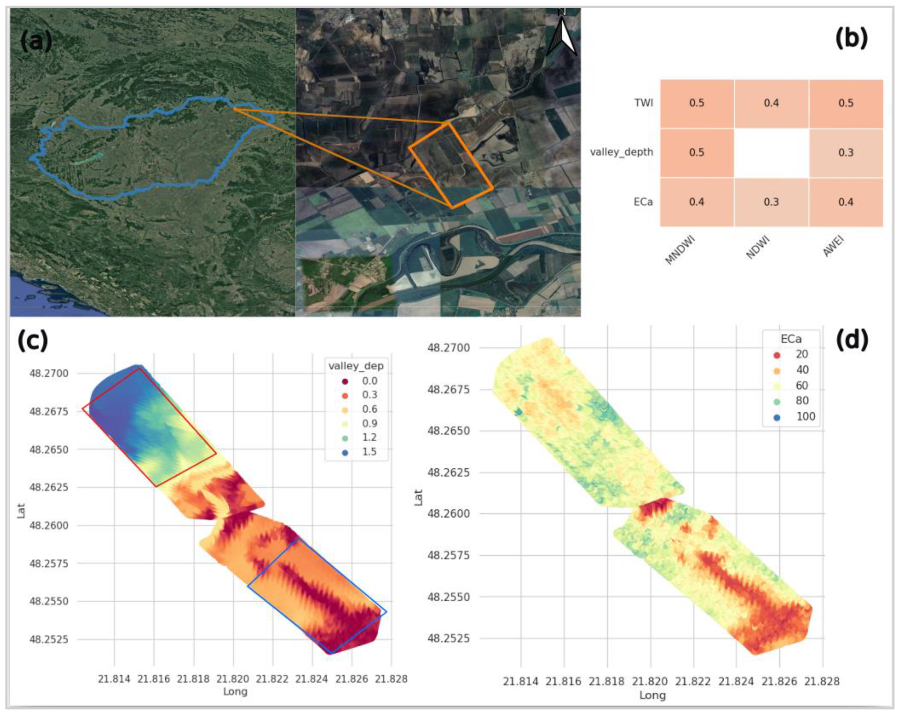
2.1. Study Area

The study site is a 66 ha agriculture field located in the northeast of Hungary, close to the border between Hungary and Slovakia (Figure 1a,b). The land use type is a rotation of sunflower and corn throughout the year. The climate in the region is classified as a moderately continental climate with cold summers. Data from nearby meteorological stations show the mean values for annual temperature (MAT) is (11.7 ± 1.8 °C) and the mean annual precipitation (MAP) is (554 ± 99.5 mm·year⁻¹) (Figure A1). According to the standardized field guide for soil description and classification, the dominant soil type is classified as Vertisol and is characterized by high activity clay content with low infiltration rates, hydraulic conductivity, and alternating swelling and shrinking processes [35,36]. Furthermore, the field is surrounded by streams, especially the northern part of the field. The field location within the landscape combined with poor physical soil properties has led to frequent water ponding (Figure A1), with only 75% of the total area of the field remaining for agricultural practices.

2.2. Data Collection and Processing

To understand the hydrogeomorphic characteristics of the field and how they are related to waterlogging in our case study, we collected high resolution topographic and multispectral imagery data for the investigated field. To achieve this, we flew over the entire field with a drone (DJI Phantom 4 RTK, DJI, Shenzhen, China) equipped with a DJI camera (DJI FC6310R, DJI, Shenzhen, China) to collect RGB images for visual field assessment (Figure A1). We then scanned the entire field and collected point clouds of elevation data and apparent electrical conductivity (ECa) (Figure A5) using a Veris U3000 (Veris Technologies, Salina, KS, USA), equipped with a John Deere Starfire 6000 Antenna. The Veris U3000 and the antenna were both attached to a John Deere Gator. Using point clouds of elevation data, we developed a digital elevation model (DEM) of the investigated field using the inverse weighted distance interpolation method (IWD) [37]. To understand the biophysical characteristics of the landscape, we extracted essential topographic indices from the DEM including field relative slope, valley depth, and topographic wetness index. We derived additional wetness indices from Sentinel-2 multispectral imagery. To do this, we downloaded analysis-ready Sentinel-2 data for February 2021 from the Google Earth Engine (GEE) platform using the JavaScript API available in GEE [38]. We then calculated a series of vegetation and water indices suitable for waterlogging detection for the investigated field, including the NDWI [11], MNDWI [12], AWEI [13], NDVI [39], and EVI [40] as described in the equations presented below. Geospatial data was processed using QGIS v3.22.

$$\mathrm{NDWI}=\frac{\mathrm{Band} 3- \mathrm{Band} 8}{\mathrm{Band} 3+ \mathrm{Band} 8}$$

$$\mathrm{MNDWI}=\frac{\mathrm{Band} 3- \mathrm{Band} 11}{\mathrm{Band} 3+ \mathrm{Band} 11}$$

$$\mathrm{AWEI}=\mathrm{Band} 8+ \mathrm{Band} 2\ast 0.25-1.5 \ast \left(\mathrm{Band} 8+ \mathrm{Band} 11\right)-0.25 \ast \mathrm{Band} 12$$

$$\mathrm{EVI}=\frac{2.5 \ast \left(\mathrm{Band} 8- \mathrm{Band} 4\right)}{\left(\mathrm{Band} 8+6.0 \ast \mathrm{Band} 4-7.5 \ast \mathrm{Band} 2\right)+1.0}$$

$$\mathrm{NDVI}=\frac{\mathrm{Band} 8- \mathrm{Band} 4}{\mathrm{Band} 8+ \mathrm{Band} 4}$$

Agricultural Production and Financial Data

In 2020, we collected data from the investigated farm including the cultivated area, actual and expected yield (i.e., in ideal conditions), and production/technology costs for corn and sunflower, the two dominant crops in the area. For our analysis, we divided the data into two management scenarios. The first scenario is referred to as “current farm management”, in which farm production and profitability is reduced with only part of the farm under operation (~75% of the total area). This is also when yield and farm activities are impaired by waterlogging. The second scenario is referred to as “application of drainage”. In this scenario, farm production and profitability benefit from the total area of the farm being under operation. This is also a scenario when soil conditions are favorable for crop production for the entire area (100%) of the farm. In this study, we assumed that this is the ideal scenario representing a well-drained field. To calculate the annual farm revenue for each crop, we used data published by the Hungarian Central Statistical Office. We calculated the farm revenue per crop per year as a product of yield (tonnes/ha) and the national average price EUR per ton per crop in the same year. We then calculated the farm profitability (benefit) as the difference between total annual income and production cost per crop per year. The available data at the farm level starts from 2018 to 2022. Therefore, to match market-published data and farm data in our analysis, we focused on 2018–2022. To account for the cost of drainage we used a reasonable value reported for EU countries (approximately 140 EUR/ha). As the technology cost and farm revenue depend on the inflation rate of the country, we collected the country’s annual inflation rates from 2018 to 2022 (published by the Hungarian Central Statistical Office and the World Bank Group data portal).

2.3. Statistical Analysis

We conducted the statistical analyses in four steps: K-means clustering for mapping waterlogging, an A/B test, a correlation analysis between the independent variables, and Bayesian modeling for decision-making. In the first step, to identify potential sites for waterlogging in the investigated field, we used an unsupervised learning technique, the K-means clustering algorithm [41,42]. K-means clustering is the partitioning algorithm that assigns each data point in the dataset to only one of the adjacent clusters using a measure of distance or similarity. K-means clustering has been identified as a simple, intuitive, and elegant approach for partitioning a dataset into K-distinct, nonoverlapping clusters. To perform K-means clustering, the user first specifies the desired number of K clusters, then the K-means algorithm assigns each observation to exactly one of the K clusters [43]. To simplify the learning and computation time in this study, we set the desired number of clusters to 2, because in our case study scenario, we expected each part of the field to fall into one of the following categories: (1) potential waterlogged sites or (2) well-drained sites. There are many unsupervised learning algorithms in the recent literature. However, we chose the K-means clustering for the following reasons: first, we chose the K-means clustering because we were interested in minimizing the within-cluster variance. Second, before conducting the analysis, our environmental covariates (i.e., predictors) were normalized, making the K-means algorithm suitable for this type of data. Finally, as we had predefined the number of clusters suitable for our problem, the K-means clustering algorithm was an ideal choice.

To evaluate the model and select the number of optimal clusters that fit our data points, we used the silhouette and elbow methods [42,44,45]. For each technique, we ran 11 iterations, with each iteration representing the number of clusters. For the first evaluation method, an average silhouette coefficient based on 11 iterations was calculated to identify the optimal number of clusters representing our data points. The entire clustering was then displayed by combining the silhouettes into a single plot, allowing an assessment of the relative quality of the clusters and an overview of the data configuration. There are many evaluation techniques for validating clustering algorithms. Since both K-means and silhouette analyses are based on Euclidian distance metrics, we decided to use the silhouette coefficient for our model evaluation to simplify and harmonize the entire analysis. In the second phase, the elbow method was used. The elbow method consists of plotting the explained variation as a function of the number of clusters and picking the elbow of the curve as the number of clusters to use. We chose the elbow method because it is widely used in other unsupervised analyses such as principal component analysis. The results of the two techniques (Figure A2) provide a robust approach for evaluating the output of our cluster analysis.

In the second step, we conducted a hypothesis analysis to test whether there is a difference between the average farm profitability before and after the implementation of the drainage system. That is, whether there is a difference in profit between the current farm management and the one after the installation of the drainage system, and whether the farmer should adopt drainage practices. To do this, we conducted an A/B test [46] followed by a bootstrap resampling technique with replacement [47]. We then ran 10,000 iterations and calculated the mean difference between farm profitability (benefit) before and after the installation of the drainage system for each iteration. We then calculated the average, median, and 95% confidence interval, and plotted them against the histogram of 10,000 simulated values. This approach provides a robust way of hypothesis-testing compared to a parametric statistical test such as analysis of variance (ANOVA), and is widely used in the business and healthcare sectors for decision-making [46,48,49].

In the third step of the analysis, we conducted a correlation analysis between the independent (explanatory) variables and the dependent (response) variables to assess whether there was a positive or negative association between the explanatory variables, representing financial and biophysical characteristics of the farm, and the response variable (profitability). As multicollinearity between independent variables was expected at this stage, we selected important variables that should be used in the final analysis (modeling). To do this, we performed a cluster of the Spearman rank-order correlations, plotted a heatmap of the correlated features, picked a threshold (in this case r ≥ 0.75) [50], and kept a single feature from each cluster. This approach served as a feature selection method to avoid the use of many variables that are collinear and meaningless for the model.

In the final stage of the analysis, we used the selected variables in a Bayesian model [51]. A final Bayesian model was then constructed to identify the relationship between explanatory variables and their overall effects (posterior effect size) on the estimated benefit (farm profitability). For model setup and assessment, we used Markov chain Monte Carlo (MCMC) algorithms set up for a total of 3000 draw iterations, using 20 separate chains with 1000 tunes, and plotted the distribution of the results together with the five variables of a boxplot. We then summarized the model results based on Bayes’s theorem as posterior distribution of the marginal effect size of explanatory variables on the response variable (benefit/profitability). These methods thus directly address the question of how new evidence should change what we believe [48,52]. All analyses were conducted using Python v3.9. The A/B and correlation tests were conducted using the basic functions available for Python. The Bayesian modeling was implemented using the PyMC [53] framework available for Python. Visualization of the model output and results were implemented using Seaborn statistical data visualization [54] and matplotlib [55] libraries for Python.

3. Results and Discussion

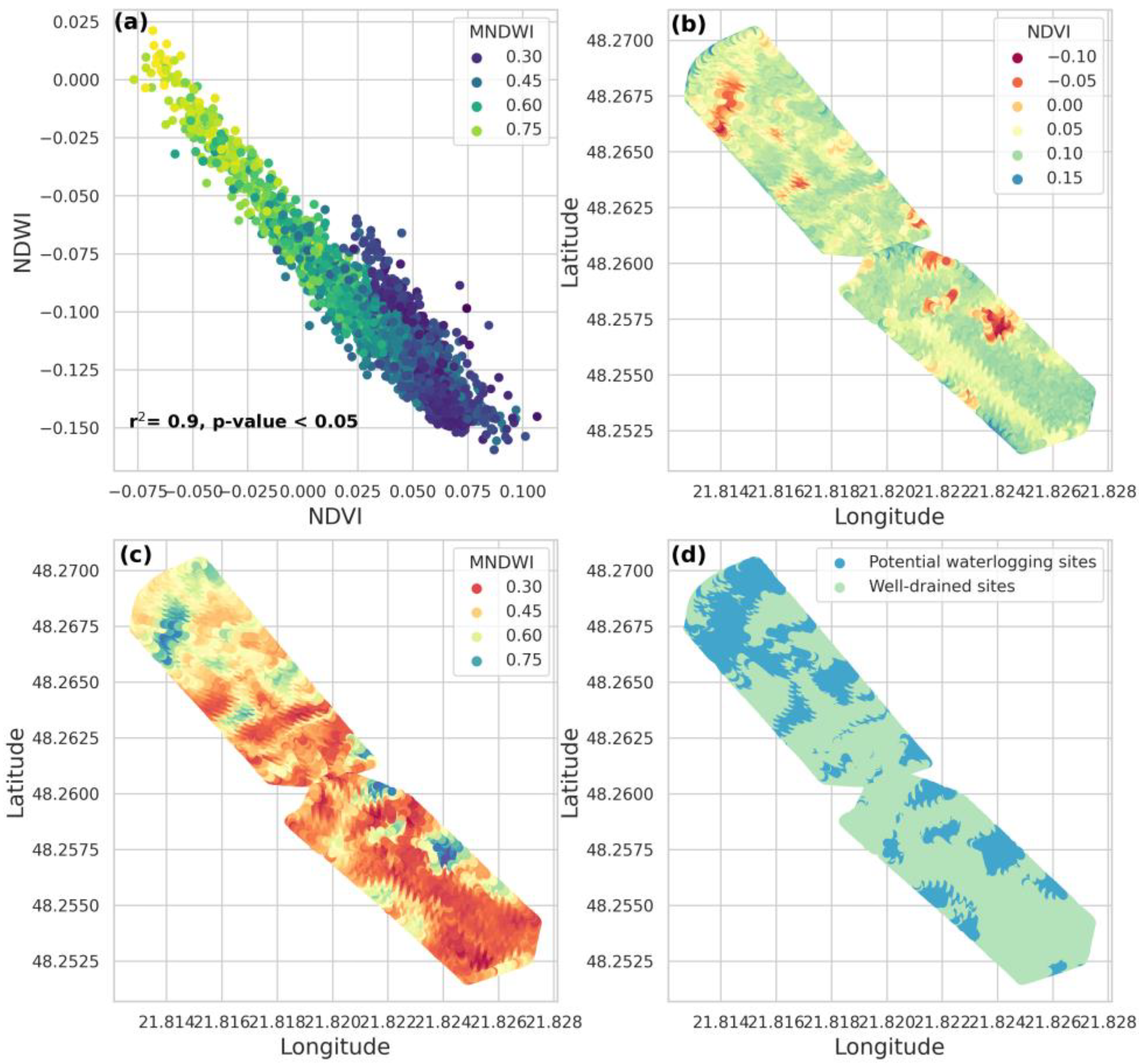
3.1. Field Hydrogeomorphic Features and Waterlogging in Agriculture

Using high-resolution remotely sensed hydrogeomorphic data, our results show that the investigated field is indeed affected by waterlogging (Figure 2a–d and Figure A1). When comparing wetness and vegetation indices, we found a strong negative correlation between the NDWI and NDVI (Figure 2a), suggesting that waterlogging has strongly impaired the yield in those spots of the farm. We also observed a significant (p-value < 0.05) positive correlation between water indices and topographic indices, especially the MNDWI (derived from Sentinel-2 imagery) and valley depth (derived from the DEM) (Figure 1b). Furthermore, our results show a significant positive correlation between the soil ECa and water indices (Figure 1b). Soil ECa is widely used to understand physico–chemical soil properties such as soil moisture conditions, soil texture, and soil pH, among others [17]. A high ECa indicates high clay content, high soil moisture, and low pH. Soil profile description data (not shown here) collected during the field campaign revealed that the waterlogged sites were indeed characterized by high clay content and low soil pH. Altogether, these results suggest that changes in soil geochemical properties driving soil water content, specifically clay content, is likely the main driver of waterlogging observed in our study field. Consequently, an increase in soil moisture created reduced conditions which further decreased soil pH. This statement is based on the fact that the observed field’s soil plasticity (estimated from soil coarseness) was higher (63–67%) in the northern part (Figure 1, red box) of the field compared to the southern part (Figure 1, blue box) of the field (32–47%). In contrast, soil pH was lower (3.5–3.6) in the northern part compared to the southern part of the field (4.5–5.2). These results have two implications for the way we plan and implement soil and water management practices. First, management practices have to be field-specific across the landscape, as well as location-based within a field, due to the high spatial variation of soil properties within fields that can influence waterlogging. Second, the implementation of soil and water management practices has to be guided by precision-farming techniques and technologies. For the latter, freely available remote sensing data combined with proximal sensing technologies and open-source algorithms can support the application of precision farming. Using a combination of three water indices (the NDWI, MNDWI, and AWEI) and two vegetation indices (the NDVI and EVI), we were able to detect and map potential sites susceptible to waterlogging (Figure 2d). The potential of these indices to detect surface water has been reported in other water-related studies [56,57,58]. For example, refs. [59,60] reported an improvement in model performance when combining the NDWI, MNDWI, AWEI, and NDVI to detect surface water. We acknowledge that the K-means methods used to detect and map waterlogging may yield some errors in the map produced due to the lack of suitable validation data. However, a study conducted in the same region as investigated here reported similarly good performance of the K-means algorithm when compared to other methods [61]. Furthermore, our analysis of model performance (the silhouette coefficient and SSE) through many iterations (Figure A2) provides a clear indication that the error associated with the generated map is likely very small. In addition, the selected vegetation (NDVI and EVI), water (NDWI, MNDWI, AWEI), and topographic indices (TWI and valley depth) together with ECa data provided further information for visual validation of the map produced (Figure 1b–d). ECa is often used to assess physical and chemical soil properties in agricultural fields and has been recently used to assess farm productivity [16,18]. However, its use for waterlogging management has not been fully explored. In summary, our results revealed the potential of vegetation and water indices to detect waterlogging even in a small-scale field. Beyond that, we show that these indices can be combined with topographic data and soil properties, such as ECa generated using proximal soil sensing technologies, to understand the drivers of waterlogging and where water management practices should precisely focus in the wave of climate change scenarios.

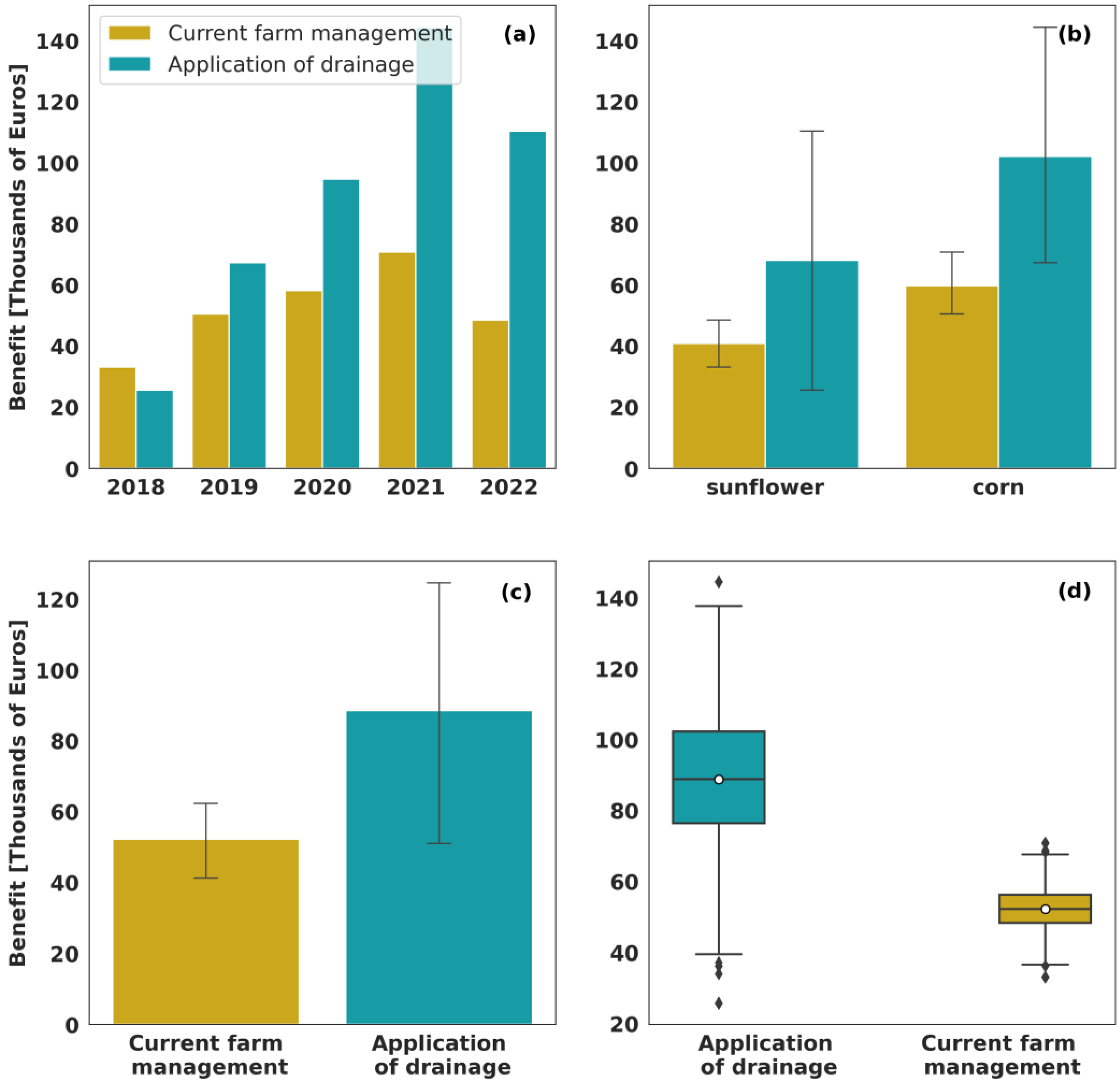
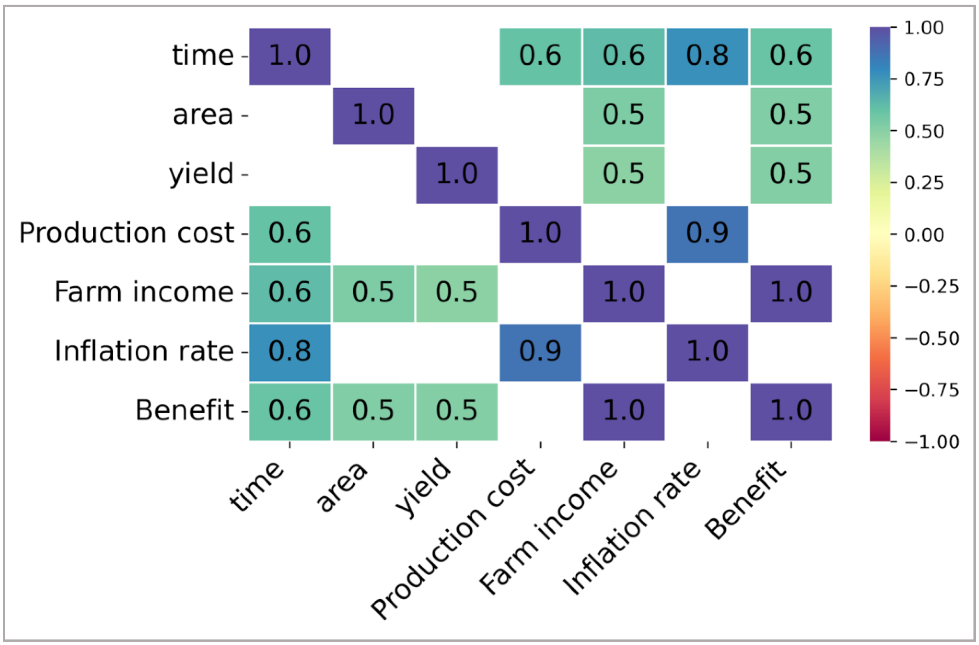
3.2. Data-Driven Decision-Making

Agriculture statistics show that for the period of four years, the estimated average annual farm production cost was (EUR 5752.4 ± 1732.5) under the current farm management scenario and (EUR 9517.9 ± 3726.7) under drainage application. The annual income was (EUR 58,020.5 ± 13,672.7) under the current farm management scenario and (EUR 99,910.6 ± 39,010.8) under drainage application. Overall, the net annual benefit was (EUR 52,268 ± 13,792.7) under the current farm management scenario and (EUR 88,544.7 ± 44,808.2) under drainage application (Figure 3a–d). Comparing the income generation for the last four years under the two scenarios, we found an increase in benefits associated with the installation of drainage from 2018 to 2022 (Figure 3a). By comparing the overall difference in benefits under current farm management and the estimated benefits under drainage application, we found a significant increase in the benefit of approximately 1.7 times associated with drainage application (Figure 3b,c and Figure A3).

The correlation analysis between farm profitability (i.e., benefit) and independent variables (cropping area, yield, and time) used in our analysis showed a significant association between farm profitability (benefit) and that set of variables (Figure 4). The analysis suggests that, over time, an extension of cropping area through the application of drainage would have boosted crop yield and the associated farm profitability (Figure 4).

Using the selected variables (i.e., cropping area, yield, and time) in a Bayesian model, we found significant positive effects between those variables and farm profitability (Figure 5a,b). The highest posterior marginal effect size was associated with time (1.95), followed by expansion of the cropping area (1.5), while the lowest was associated with yield (0.5) (Figure 5a,b). These results suggest that an increase in one unit cropping area (1 ha) through the application of drainage would have increased farm profitability (i.e., benefit) by 1.5 times compared to the current farm management scenario (Figure 5a,b). Note that time (year) represents all factors that vary with time, including weather patterns, inflation rates, and cost of production. We plotted the probability distribution of the posterior effects of the three variables and found that the likelihood of having a positive benefit was approximately 85% (Figure 5b).

Altogether, field observations and farm management data combined with statistical tools provide evidence that investing in drainage systems would yield a positive impact on farm profitability (Figure 5a). However, statistical analyses (an A/B test and the Bayesian model) revealed a large deviation in the model estimates (Figure 5 and Figure A3). The difference in benefits between current farm management and after the application of the drainage system inferred from the A/B test varied between −5.0–14.8. This wide range of estimates hints towards multiple factors that can vary at spatial and temporal scales [20,24,33]. First, we acknowledge that the uncertainty and the wide confidence interval around these estimates might be associated with other factors which were not taken into account in our Bayesian model. For example, the effects associated with climate parameters such as drought events that can affect yield. Recent research conducted in the same region as investigated here has shown that climate accounted for 17–39% of yield variability over the past 90 years, and this figure has reached 33–67% in the past 30 years. The authors reported that the impact of climate parameters to yield variability was much stronger compared to their counterpart socio–economic factors that affected the region for the last three decades [62,63].

Nonetheless, the fact that our model included time (i.e., years) as an explanatory variable that can represent other factors such as climate parameters (i.e., temperature and precipitation) or socio–economic indicators (i.e., inflation rates), we argue that the observed difference (Figure 3c,d and Figure A3) and the size of the posterior effects (Figure 5) is indeed significant and likely to occur. This statement is based on the significant positive correlation observed in our data between time, inflation rate, production cost (Figure 4), and variability of climate parameters over time (Figure A1). In line with our results, the use of time as a confounding factor has been used in other studies for decision-making [64]. The average difference observed from our A/B test results and the posterior effect size estimated using the Bayesian model (Figure 5 and Figure A3) provide evidence that the benefit associated with the application of drainage is indeed positive and the model results reflect the observed data (Figure A4). Consequently, our results evaluate a drainage project as a successful investment. Therefore, the adoption of drainage as a water management practice is likely to increase farm income and profitability in the investigated agricultural field.

In summary, agriculture scientists and resource managers are experiencing advances in agricultural technologies, often related to precision farming. However, each individual tool is used in an isolated manner without a clear connection. For example, in agriculture, especially water management, research often focuses on monitoring with limited research on management and decision-making. This study attempted to connect different approaches to support decision-making in the agriculture sector, from monitoring, to planning, to decision-making. This study revealed that the combination of remotely sensed data, Bayesian modeling, and A/B testing presents a promising area for future research in agriculture resource management. Combining these tools can provide a deep understanding of the impact of waterlogging on farm production and productivity, as well as on the cost–benefit ratio. As more freely available data, data collection, and analytical tools emerge, there is great potential for these methods to significantly contribute to sustainable water and agriculture management. Furthermore, this study opens up questions that are worthy of further investigation: (1) It is not clear how different factors interact to influence decision-making specifically for water management, but also in agricultural resource management. Here, a combination of Bayesian network and causal inference can provide further insights. (2) There is a need to integrate multiple data sources such as social, environmental, and economic aspects of farmers with long-term datasets, and quantify uncertainties associated with each factor which can improve the accuracy and reliability of predictions related to waterlogging management and other agricultural challenges.

4. Conclusions

The results of this study suggest strong associations between vegetation indices, water indices, ECa, and susceptibility to waterlogging. This adds substantial and understudied complexity that needs to be unraveled to better understand the relationship between hydrogeochemical features and waterlogging in agroecosystems. Furthermore, this study highlights potential data-driven methods to assess and plan agricultural projects. This is essential in the agricultural sector where project implementation is often associated with risk and uncertainty. The study shows that a combination of remote sensing and proximal sensing data can accurately map potential waterlogging sites, even at the farm scale. Using an unsupervised machine learning approach (K-means), our results revealed that waterlogging follows patterns related to three water indices (the NDWI, MNDWI, and AWEI) and two vegetation indices (the NDVI and EVI). The sensitivity of these indices is driven by edaphic factors such as ECa. The results revealed that differences in soil ECa, likely as a result of change in soil texture, had a substantial effect on waterlogging in the investigated sites. The study further shows the potential of statistical tools such as A/B testing and Bayesian statistics to support decision-making for agricultural project planning. The results of this study hint towards opportunities for future work, which could explore the available approaches to assess cost-effective methods for agricultural project assessment and planning under multiple uncertain scenarios.

References

1. Lebay, M.; Abiye, W.; Taye, T.; Belay, S. Evaluation of Soil Drainage Methods for the Productivity of Waterlogged Vertisols in Jama District, Eastern Amhara Region, Ethiopia. Int. J. Agron. 2021, 2021, e5534866. [Google Scholar] [CrossRef]
2. Pais, I.P.; Moreira, R.; Semedo, J.N.; Ramalho, J.C.; Lidon, F.C.; Coutinho, J.; Maçãs, B.; Scotti-Campos, P. Wheat Crop under Waterlogging: Potential Soil and Plant Effects. Plants 2023, 12, 149. [Google Scholar] [CrossRef] [PubMed]
3. Li, Y.; Shao, M. Effects of rainfall intensity on rainfall infiltration and redistribution in soil on Loess slope land. Ying Yong Sheng Tai Xue Bao 2006, 17, 2271–2276. [Google Scholar] [PubMed]
4. Várallyay, G. Soils, as the most important natural resources in Hungary (potentialities and constraints)—A review. Agrokémia És Talajt. 2015, 64, 321–338. [Google Scholar] [CrossRef] [Green Version]
5. Den Besten, N.; Steele-Dunne, S.; de Jeu, R.; van der Zaag, P. Towards Monitoring Waterlogging with Remote Sensing for Sustainable Irrigated Agriculture. Remote Sens. 2021, 13, 2929. [Google Scholar] [CrossRef]
6. Kabała, C.; Charzyński, P.; Czigány, S.; Novák, T.J.; Saksa, M.; Świtoniak, M. Suitability of World Reference Base for Soil Resources (WRB) to Describe and Classify Chernozemic Soils in Central Europe. Soil Sci. Annu. 2019, 70, 244–257. [Google Scholar] [CrossRef]
7. Tilahun, T.; Seyoum, W.M. High-Resolution Mapping of Tile Drainage in Agricultural Fields Using Unmanned Aerial System (UAS)-Based Radiometric Thermal and Optical Sensors. Hydrology 2021, 8, 2. [Google Scholar] [CrossRef]
8. Rahman, M.M.; Chakraborty, T.K.; Al Mamun, A.; Kiaya, V. Land- and Water-Based Adaptive Farming Practices to Cope with Waterlogging in Variably Elevated Homesteads. Sustainability 2023, 15, 2087. [Google Scholar] [CrossRef]
9. Singh, S.K.; Pandey, A.C. Geomorphology and the Controls of Geohydrology on Waterlogging in Gangetic Plains, North Bihar, India. Environ. Earth Sci. 2014, 71, 1561–1579. [Google Scholar] [CrossRef]
10. Al-Maliki, S.; Ibrahim, T.I.M.; Jakab, G.; Masoudi, M.; Makki, J.S.; Vekerdy, Z. An Approach for Monitoring and Classifying Marshlands Using Multispectral Remote Sensing Imagery in Arid and Semi-Arid Regions. Water 2022, 14, 1523. [Google Scholar] [CrossRef]
11. McFEETERS, S.K. The Use of the Normalized Difference Water Index (NDWI) in the Delineation of Open Water Features. Int. J. Remote Sens. 1996, 17, 1425–1432. [Google Scholar] [CrossRef]
12. Xu, H. Modification of Normalised Difference Water Index (NDWI) to Enhance Open Water Features in Remotely Sensed Imagery. Int. J. Remote Sens. 2006, 27, 3025–3033. [Google Scholar] [CrossRef]
13. Feyisa, G.L.; Meilby, H.; Fensholt, R.; Proud, S.R. Automated Water Extraction Index: A New Technique for Surface Water Mapping Using Landsat Imagery. Remote Sens. Environ. 2014, 140, 23–35. [Google Scholar] [CrossRef]
14. Fei, X.; Li, Y.-Z.; Du, Y.; Ling, F.; Yan, Y.; Feng, Q.; Ban, X. Monitoring Perennial Sub-Surface Waterlogged Croplands Based on MODIS in Jianghan Plain, Middle Reaches of the Yangtze River. J. Integr. Agric. 2014, 13, 1791–1801. [Google Scholar]
15. Ibrahim, T.I.M.; Al-Maliki, S.; Salameh, O.; Waltner, I.; Vekerdy, Z. Improving LST Downscaling Quality on Regional and Field-Scale by Parameterizing the DisTrad Method. ISPRS Int. J. Geo-Inf. 2022, 11, 327. [Google Scholar] [CrossRef]
16. Corwin, D.L.; Lesch, S.M. Application of Soil Electrical Conductivity to Precision Agriculture. Agron. J. 2003, 95, 455–471. [Google Scholar] [CrossRef]
17. Kinoshita, R.; Tani, M.; Sherpa, S.; Ghahramani, A.; van Es, H.M. Soil Sensing and Machine Learning Reveal Factors Affecting Maize Yield in the Mid-Atlantic United States. Agron. J. 2023, 115, 181–196. [Google Scholar] [CrossRef]
18. Lu, S.G.; Tang, C.; Rengel, Z. Combined Effects of Waterlogging and Salinity on Electrochemistry, Water-Soluble Cations and Water Dispersible Clay in Soils with Various Salinity Levels. Plant Soil 2004, 264, 231–245. [Google Scholar] [CrossRef]
19. Valayamkunnath, P.; Barlage, M.; Chen, F.; Gochis, D.J.; Franz, K.J. Mapping of 30-Meter Resolution Tile-Drained Croplands Using a Geospatial Modeling Approach. Sci. Data 2020, 7, 257. [Google Scholar] [CrossRef]
20. Yet, B.; Lamanna, C.; Shepherd, K.D.; Rosenstock, T.S. Evidence-Based Investment Selection: Prioritizing Agricultural Development Investments under Climatic and Socio-Political Risk Using Bayesian Networks. PLoS ONE 2020, 15, e0234213. [Google Scholar] [CrossRef]
21. Pollino, C.A.; Woodberry, O.; Nicholson, A.; Korb, K.; Hart, B.T. Parameterisation and Evaluation of a Bayesian Network for Use in an Ecological Risk Assessment. Environ. Model. Softw. 2007, 22, 1140–1152. [Google Scholar] [CrossRef]
22. Barton, D.N.; Saloranta, T.; Moe, S.J.; Eggestad, H.O.; Kuikka, S. Bayesian Belief Networks as a Meta-Modelling Tool in Integrated River Basin Management—Pros and Cons in Evaluating Nutrient Abatement Decisions under Uncertainty in a Norwegian River Basin. Ecol. Econ. 2008, 66, 91–104. [Google Scholar] [CrossRef]
23. Freebairn, J.W. Assessing Some Effects of Inflation on the Agricultural Sector. Aust. J. Agric. Econ. 1981, 25, 107–122. [Google Scholar] [CrossRef] [Green Version]
24. Yet, B.; Constantinou, A.; Fenton, N.; Neil, M.; Luedeling, E.; Shepherd, K. A Bayesian Network Framework for Project Cost, Benefit and Risk Analysis with an Agricultural Development Case Study. Expert Syst. Appl. 2016, 60, 141–155. [Google Scholar] [CrossRef]
25. Puga, J.L.; Krzywinski, M.; Altman, N. Bayesian Statistics. Nat. Methods 2015, 12, 377–378. [Google Scholar] [CrossRef]
26. Vogelgesang, J.; Scharkow, M. Bayesian Statistics. In The International Encyclopedia of Communication Research Methods; John Wiley & Sons, Ltd.: Hoboken, NJ, USA, 2017; pp. 1–9. ISBN 978-1-118-90173-1. [Google Scholar]
27. Van de Schoot, R.; Depaoli, S.; King, R.; Kramer, B.; Märtens, K.; Tadesse, M.G.; Vannucci, M.; Gelman, A.; Veen, D.; Willemsen, J.; et al. Bayesian Statistics and Modelling. Nat. Rev. Methods Prim. 2021, 1, 1. [Google Scholar] [CrossRef]
28. Flaxman, S.; Mishra, S.; Gandy, A.; Unwin, H.J.T.; Mellan, T.A.; Coupland, H.; Whittaker, C.; Zhu, H.; Berah, T.; Eaton, J.W.; et al. Estimating the Effects of Non-Pharmaceutical Interventions on COVID-19 in Europe. Nature 2020, 584, 257–261. [Google Scholar] [CrossRef]
29. Brauner, J.M.; Mindermann, S.; Sharma, M.; Johnston, D.; Salvatier, J.; Gavenčiak, T.; Stephenson, A.B.; Leech, G.; Altman, G.; Mikulik, V.; et al. Inferring the Effectiveness of Government Interventions against COVID-19. Science 2021, 371, eabd9338. [Google Scholar] [CrossRef]
30. Govender, I.H.; Sahlin, U.; O’Brien, G.C. Bayesian Network Applications for Sustainable Holistic Water Resources Management: Modeling Opportunities for South Africa. Risk Anal. 2022, 42, 1346–1364. [Google Scholar] [CrossRef]
31. Cornet, D.; Sierra, J.; Tournebize, R.; Gabrielle, B.; Lewis, F.I. Bayesian Network Modeling of Early Growth Stages Explains Yam Interplant Yield Variability and Allows for Agronomic Improvements in West Africa. Eur. J. Agron. 2016, 75, 80–88. [Google Scholar] [CrossRef]
32. Rasmussen, S.; Madsen, A.L.; Lund, M. Bayesian Network as a Modelling Tool for Risk Management in Agriculture; IFRO Working Paper; University of Copenhagen, Department of Food and Resource Economics (IFRO): Copenhagen, Denmark, 2013. [Google Scholar]
33. Constantinou, A.C.; Fenton, N.; Neil, M. Integrating Expert Knowledge with Data in Bayesian Networks: Preserving Data-Driven Expectations When the Expert Variables Remain Unobserved. Expert Syst. Appl. 2016, 56, 197–208. [Google Scholar] [CrossRef]
34. Tari, F. A Bayesian Network for Predicting Yield Response of Winter Wheat to Fungicide Programmes. Comput. Electron. Agric. 1996, 15, 111–121. [Google Scholar] [CrossRef]
35. IUSS Working Group WRB World Reference Base for Soil Resources 2014, Update 2015 International Soil Classification System for Naming Soils and Creating Legends for Soil Maps; World Soil Resources Reports No. 106; FAO: Roma, Italy, 2015.
36. FAO. Guidelines for Soil Description; FAO: Roma, Italy, 2006. [Google Scholar]
37. Shepard, D. A Two-Dimensional Interpolation Function for Irregularly-Spaced Data. In Proceedings of the 1968 23rd ACM National Conference, New York, NY, USA, 27–29 August 1968; Association for Computing Machinery: New York, NY, USA, 1968; pp. 517–524. [Google Scholar]
38. Gorelick, N.; Hancher, M.; Dixon, M.; Ilyushchenko, S.; Thau, D.; Moore, R. Google Earth Engine: Planetary-Scale Geospatial Analysis for Everyone. Remote Sens. Environ. 2017, 202, 18–27. [Google Scholar] [CrossRef]
39. Crippen, R.E. Calculating the Vegetation Index Faster. Remote Sens. Environ. 1990, 34, 71–73. [Google Scholar] [CrossRef]
40. Huete, A.; Didan, K.; Miura, T.; Rodriguez, E.P.; Gao, X.; Ferreira, L.G. Overview of the Radiometric and Biophysical Performance of the MODIS Vegetation Indices. Remote Sens. Environ. 2002, 83, 195–213. [Google Scholar] [CrossRef]
41. Pelleg, D.; Moore, A. Accelerating Exact K-Means Algorithms with Geometric Reasoning. In Proceedings of the Fifth ACM SIGKDD International Conference on KNOWLEDGE Discovery and Data Mining, San Diego, CA, USA, 15–18 August 1999; Association for Computing Machinery: New York, NY, USA, 1999; pp. 277–281. [Google Scholar]
42. Goutte, C.; Hansen, L.K.; Liptrot, M.G.; Rostrup, E. Feature-Space Clustering for FMRI Meta-Analysis. Hum Brain Mapp 2001, 13, 165–183. [Google Scholar] [CrossRef]
43. James, G.; Witten, D.; Hastie, T.; Tibshirani, R. Unsupervised Learning. In An Introduction to Statistical Learning: With Applications in R; Springer Texts in Statistics; James, G., Witten, D., Hastie, T., Tibshirani, R., Eds.; Springer: New York, NY, USA, 2013; pp. 373–418. ISBN 978-1-4614-7138-7. [Google Scholar]
44. Thorndike, R.L. Who Belongs in the Family? Psychometrika 1953, 18, 267–276. [Google Scholar] [CrossRef]
45. Rousseeuw, P.J. Silhouettes: A Graphical Aid to the Interpretation and Validation of Cluster Analysis. J. Comput. Appl. Math. 1987, 20, 53–65. [Google Scholar] [CrossRef] [Green Version]
46. Kohavi, R.; Longbotham, R. Online Controlled Experiments and A/B Testing. In Encyclopedia of Machine Learning and Data Mining; Sammut, C., Webb, G.I., Eds.; Springer US: Boston, MA, USA, 2017; pp. 922–929. ISBN 978-1-4899-7687-1. [Google Scholar]
47. Efron, B.; Tibshirani, R.J. An Introduction to the Bootstrap; Chapman and Hall/CRC: New York, NY, USA, 1994; ISBN 978-0-429-24659-3. [Google Scholar]
48. Spiegelhalter, D.J.; Myles, J.P.; Jones, D.R.; Abrams, K.R. Bayesian Methods in Health Technology Assessment: A Review. Health Technol Assess 2000, 4, 1–130. [Google Scholar] [CrossRef] [Green Version]
49. Kohavi, R.; Longbotham, R.; Sommerfield, D.; Henne, R.M. Controlled Experiments on the Web: Survey and Practical Guide. Data Min. Knowl. Disc. 2009, 18, 140–181. [Google Scholar] [CrossRef] [Green Version]
50. Kuhn, M.; Johnson, K. Applied Predictive Modeling; Springer: New York, NY, USA, 2013; ISBN 978-1-4614-6848-6. [Google Scholar]
51. Gleason, P.M.; Harris, J.E. The Bayesian Approach to Decision Making and Analysis in Nutrition Research and Practice. J. Acad. Nutr. Diet. 2019, 119, 1993–2003. [Google Scholar] [CrossRef] [PubMed]
52. Harrell, F.E.; Shih, Y.C. Using Full Probability Models to Compute Probabilities of Actual Interest to Decision Makers. Int. J. Technol. Assess. Health Care 2001, 17, 17–26. [Google Scholar] [CrossRef] [PubMed]
53. Salvatier, J.; Wiecki, T.V.; Fonnesbeck, C. Probabilistic Programming in Python Using PyMC3. PeerJ Comput. Sci. 2016, 2, e55. [Google Scholar] [CrossRef] [Green Version]
54. Waskom, M.L. Seaborn: Statistical Data Visualization. J. Open Source Softw. 2021, 6, 3021. [Google Scholar] [CrossRef]
55. Hunter, J.D. Matplotlib: A 2D Graphics Environment. Comput. Sci. Eng. 2007, 9, 90–95. [Google Scholar] [CrossRef]
56. Zhang, M.; Liu, D.; Wang, S.; Xiang, H.; Zhang, W. Multisource Remote Sensing Data-Based Flood Monitoring and Crop Damage Assessment: A Case Study on the 20 July 2021 Extraordinary Rainfall Event in Henan, China. Remote Sens. 2022, 14, 5771. [Google Scholar] [CrossRef]
57. Tran, K.H.; Menenti, M.; Jia, L. Surface Water Mapping and Flood Monitoring in the Mekong Delta Using Sentinel-1 SAR Time Series and Otsu Threshold. Remote Sens. 2022, 14, 5721. [Google Scholar] [CrossRef]
58. Șerban, C.; Maftei, C.; Dobrică, G. Surface Water Change Detection via Water Indices and Predictive Modeling Using Remote Sensing Imagery: A Case Study of Nuntasi-Tuzla Lake, Romania. Water 2022, 14, 556. [Google Scholar] [CrossRef]
59. Acharya, T.D.; Subedi, A.; Lee, D.H. Evaluation of Water Indices for Surface Water Extraction in a Landsat 8 Scene of Nepal. Sensors 2018, 18, 2580. [Google Scholar] [CrossRef] [Green Version]
60. Pang, H.; Wang, X.; Hou, R.; You, W.; Bian, Z.; Sang, G. Multiwater Index Synergistic Monitoring of Typical Wetland Water Bodies in the Arid Regions of West-Central Ningxia over 30 Years. Water 2023, 15, 20. [Google Scholar] [CrossRef]
61. Gulácsi, A.; Kovács, F. Sentinel-1-Imagery-Based High-Resolution Water Cover Detection on Wetlands, Aided by Google Earth Engine. Remote Sens. 2020, 12, 1614. [Google Scholar] [CrossRef]
62. Buzási, A.; Pálvölgyi, T.; Esses, D. Drought-Related Vulnerability and Its Policy Implications in Hungary. Mitig Adapt Strat. Glob Change 2021, 26, 11. [Google Scholar] [CrossRef]
63. Pinke, Z.; Lövei, G.L. Increasing Temperature Cuts Back Crop Yields in Hungary over the Last 90 Years. Glob. Change Biol. 2017, 23, 5426–5435. [Google Scholar] [CrossRef] [PubMed]
64. Jäger, F.; Rudnick, J.; Lubell, M.; Kraus, M.; Müller, B. Using Bayesian Belief Networks to Investigate Farmer Behavior and Policy Interventions for Improved Nitrogen Management. Environ. Manag. 2022, 69, 1153–1166. [Google Scholar] [CrossRef]
Figure 1. (a) Overview map of the study region with google satellite image in the background. The blue color boundary indicates the country’s (Hungary) border, and the orange rectangle indicates the location of the investigated field. (b) Pearson correlation coefficients among hydrogeomorphic parameters of the investigated field. Blank cells indicate non-significant correlations, p  ≤  0.05. (c) Valley depth distribution of the field as a topographic feature influencing water flows across the field. The red and blue rectangles indicate the upper and lower parts of the field, respectively. (d) Map of the apparent electrical conductivity of the investigated field.
Water 15 01340 g001
Figure 2. Spatial distribution of vegetation and water indices used to detect waterlogging patterns in the investigated field. (a) Relationship between NDVI, NDWI, and MNDWI. Note the strong negative correlation between NDVI and the two water indices. (b) Spatial patterns of NDVI. (c) Spatial distribution of MNDWI for the investigated field. The dark blue color indicates high values of MNDWI and potential waterlogging sites. (d) Map of waterlogging detected across the field, using a combination of water and vegetation indices and the K-means algorithm.
Water 15 01340 g002
Figure 3. Distribution of farm income as a benefit, presented in Hungarian forint (local currency). (a) Data presented per year from 2018 to 2022 for the current farm management scenario (i.e., in the absence of drainage application) and the expected scenario (i.e., if drainage is applied), (b) data grouped per crop type, (c) the overall difference (mean ± sd) between the actual and the expected benefit after drainage, and (d) the distribution of actual and estimated benefit after drainage application. In panels (c,d), data is based on 10,000 simulations conducted using the A/B test. The white dots in the boxplot represent the average benefit over a period of four years. The points in diamond shape outside the lower and upper whiskers of the boxplot indicate possible outliers as a result of multiple simulations.
Water 15 01340 g003
Figure 4. Pearson correlations between variables used in the Bayesian model. The variables represent the financial income and physical characteristics of the farm. Blank cells represent non-significant correlations at p-value < 0.05.
Water 15 01340 g004
Figure 5. Distribution of posterior marginal effects size of explanatory variables used in the Bayesian model. (a) The violin plot shows the distribution of the complete data and the white dot represents the mean effect with 94% confidence. (b) The empirical cumulative distribution functions (ECDF) of the three variables with the corresponding probability of having a positive effect on farm profitability.
Water 15 01340 g005
Disclaimer/Publisher’s Note: The statements, opinions and data contained in all publications are solely those of the individual author(s) and contributor(s) and not of MDPI and/or the editor(s). MDPI and/or the editor(s) disclaim responsibility for any injury to people or property resulting from any ideas, methods, instructions or products referred to in the content.