
Debris Flow Scale Prediction Based on Correlation Analysis and Improved Support Vector Machine
Abstract
:1. Introduction
- Small debris flow refers to the amount of loose solid material flushed out if less than 10,000 cubic meters.
- Medium-sized debris flow refers to the volume of loose solid materials flushed out between 10,000 cubic meters and 100,000 cubic meters.
- Large debris flow refers to the volume of loose solid materials flushed out between 100,000 cubic meters and 1 million cubic meters.
- Giant debris flow refers to the amount of loose solid material washed out if more than 1 million cubic meters.
2. Method
2.1. Spearman Correlation Analysis
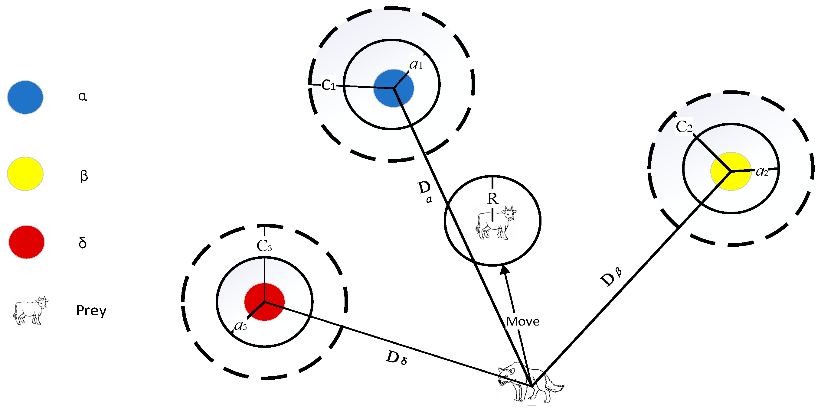
2.2. Grey Wolf Optimization Algorithm
2.3. Levi Flight Improved Grey Wolf Optimization Algorithm
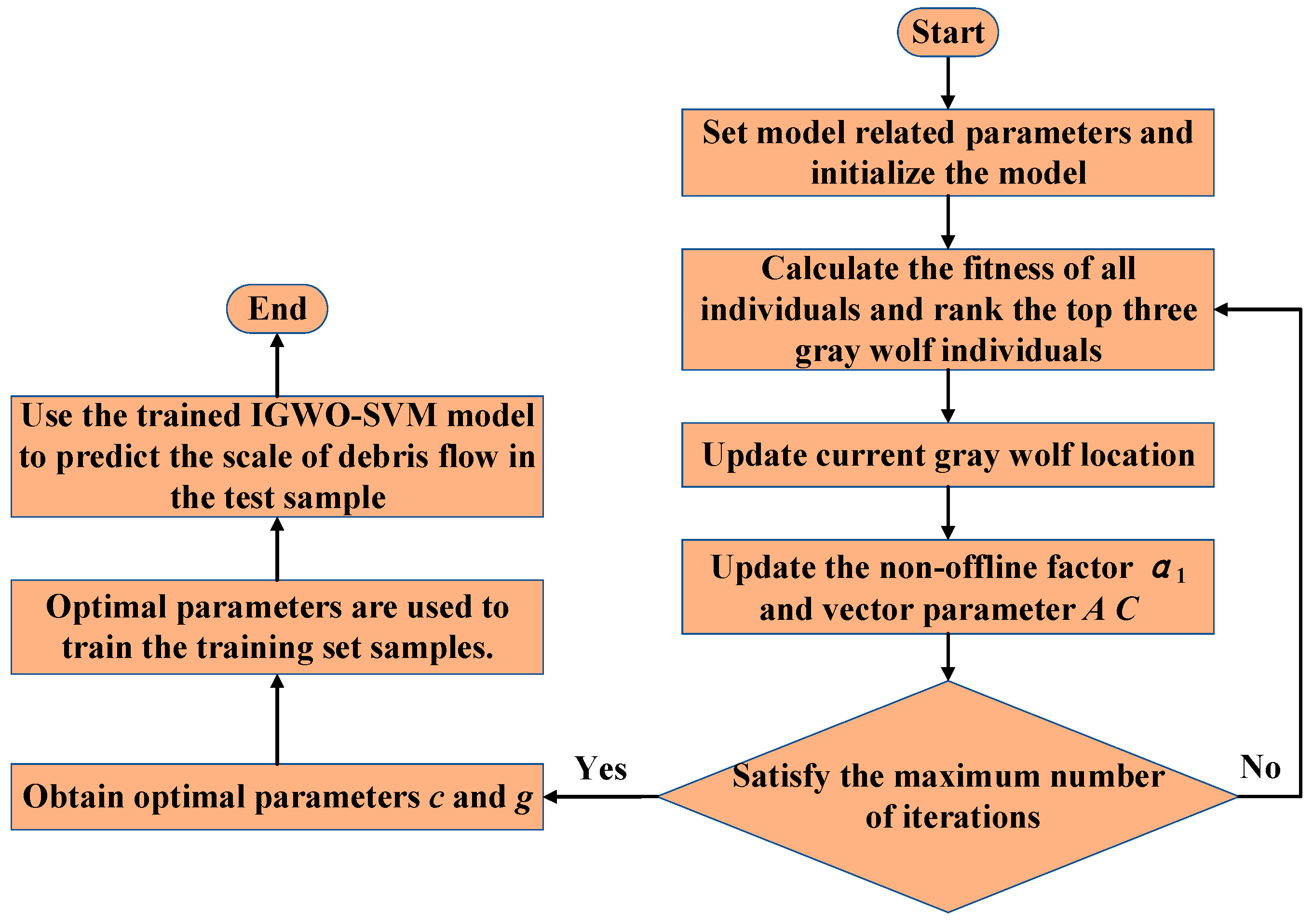
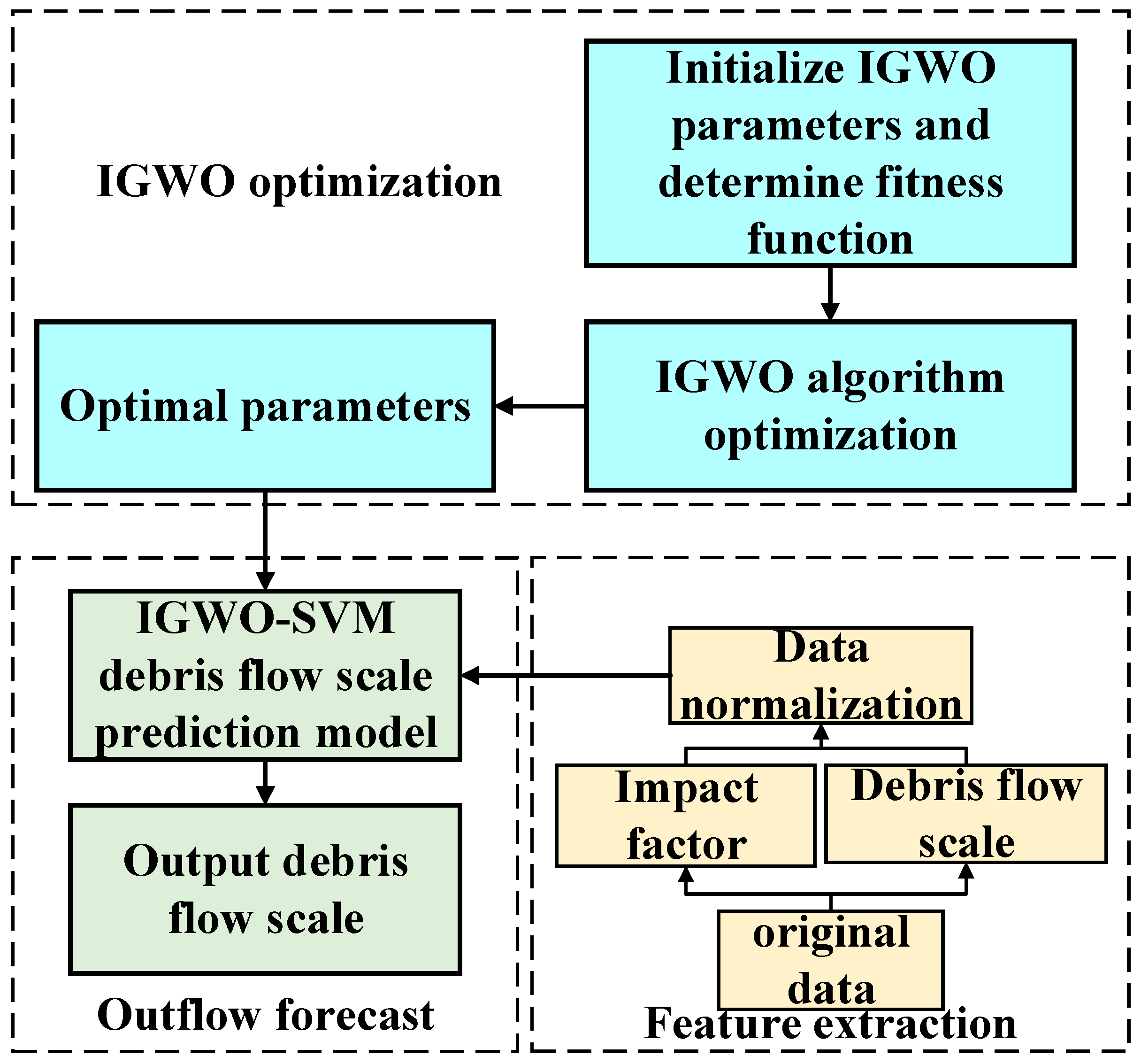
2.4. Debris Flow Outburst Scale Prediction Model Based on IGWO-SVM
- Step 1: Set the parameters of IGWO and SVM algorithms and initialize the grey wolf population.
- Step 2: Use the minimum recognition error rate of SVM for training set samples as the fitness function, calculate the fitness of all individuals in the population, and sort according to the size of the fitness value to determine the top three grey wolves.
- Step 3: Update the current position of the grey wolf individual according to Equations (10) and (12).
- Step 4: Update the value of the nonlinear convergence factor a according to Equation (13), and update the parameter vectors A and C according to Equations (8) and (9).
- Step 5: Introduce the Levy flight strategy to the grey wolf population according to Equation (14) and adjust the position of the grey wolf.
- Step 6: Determine whether the algorithm has reached the maximum number of iterations. If it is reached, the position of wolf a is returned as the optimal parameter value of SVM. If it is not reached, skip to step 2.
- Step 7: Use the optimal penalty factor c and kernel function parameter g to train and learn the training set samples to obtain the IGWO-SVM fault diagnosis model.
- Step 8: Input the test set samples into the trained IGWO-SVM model to predict the scale of debris flow outburst.
2.5. Back Propagation Neural Network
3. Application Research and Method Comparison
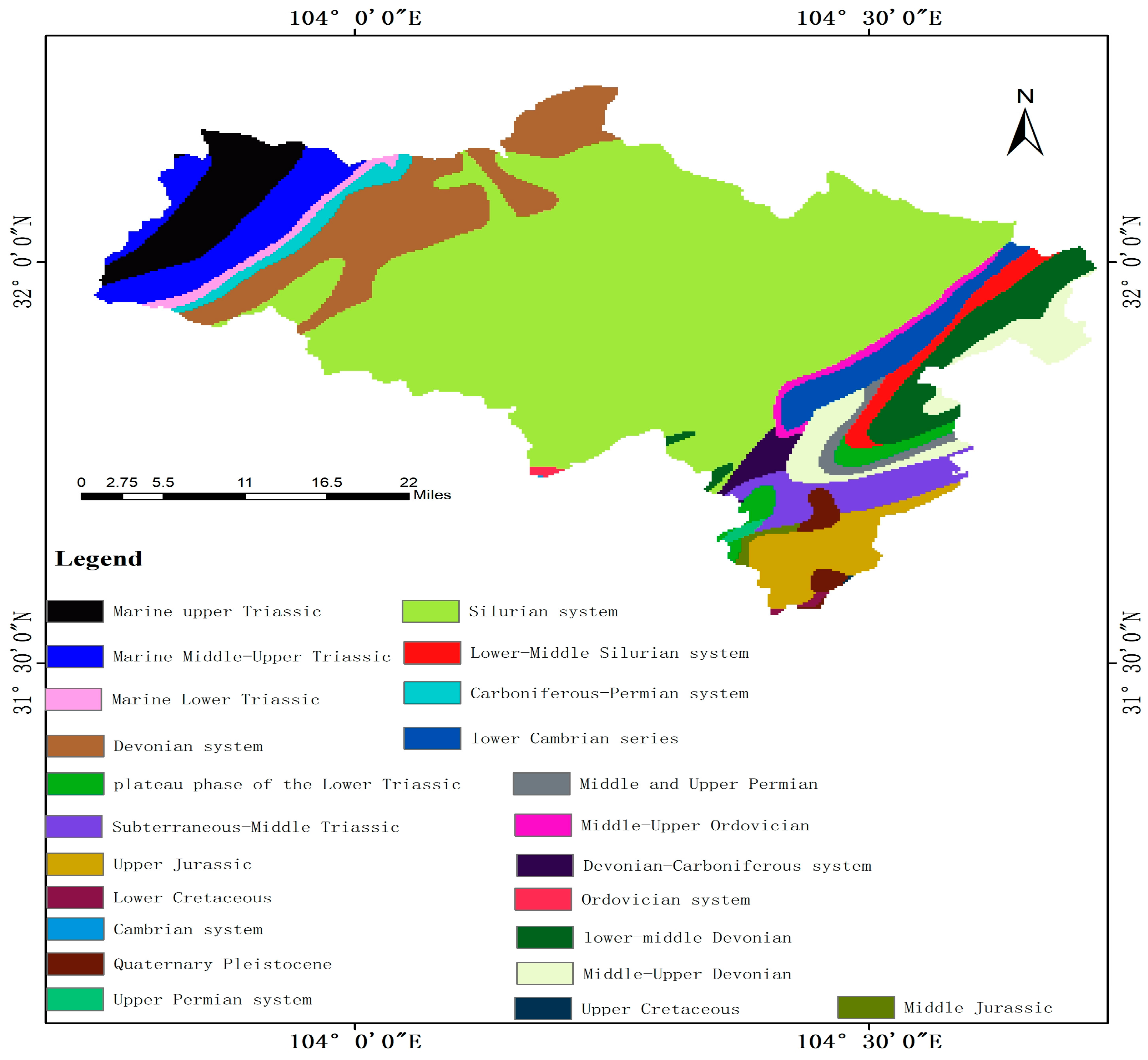
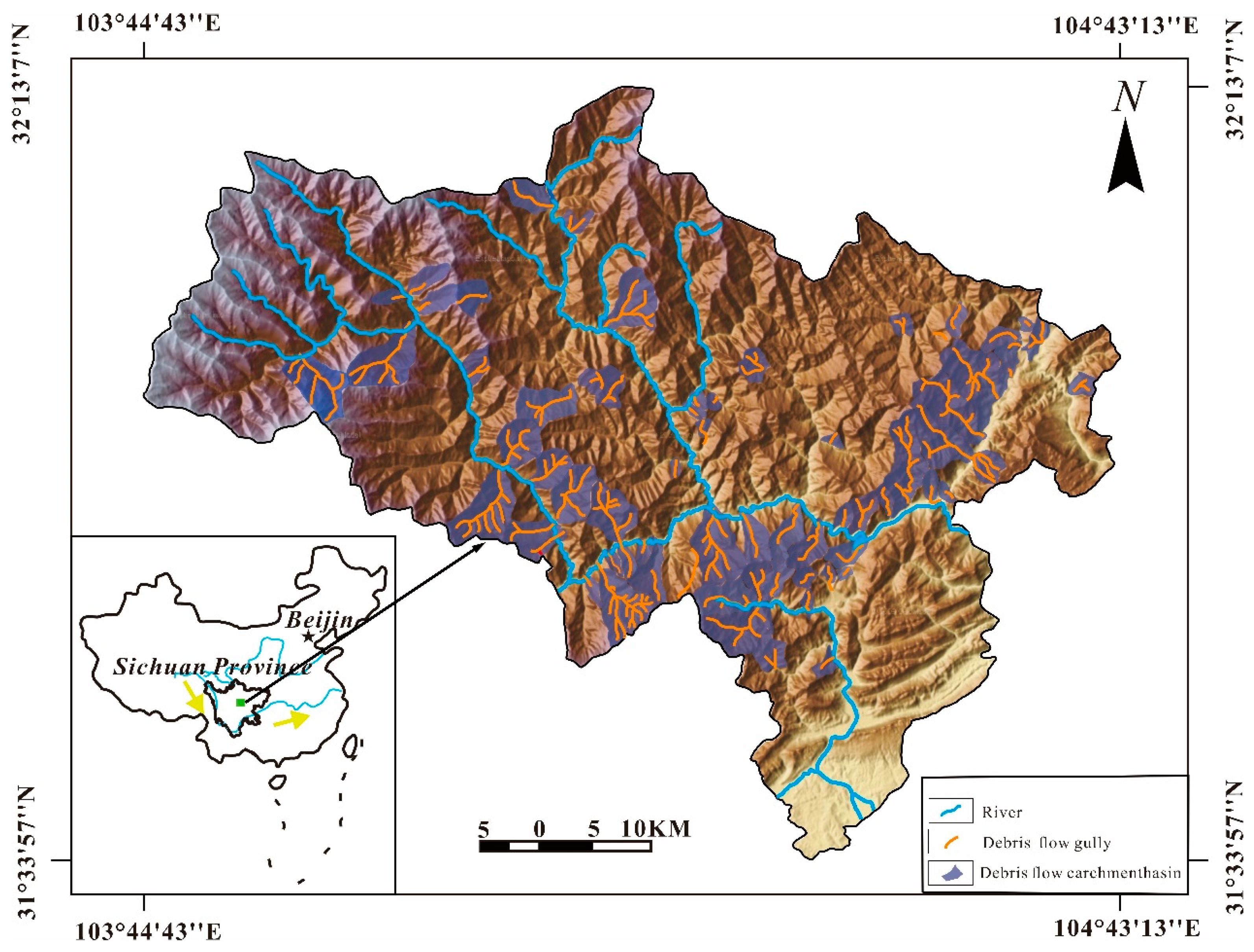
3.1. Introduction to Geology and Hydrology of Study Area
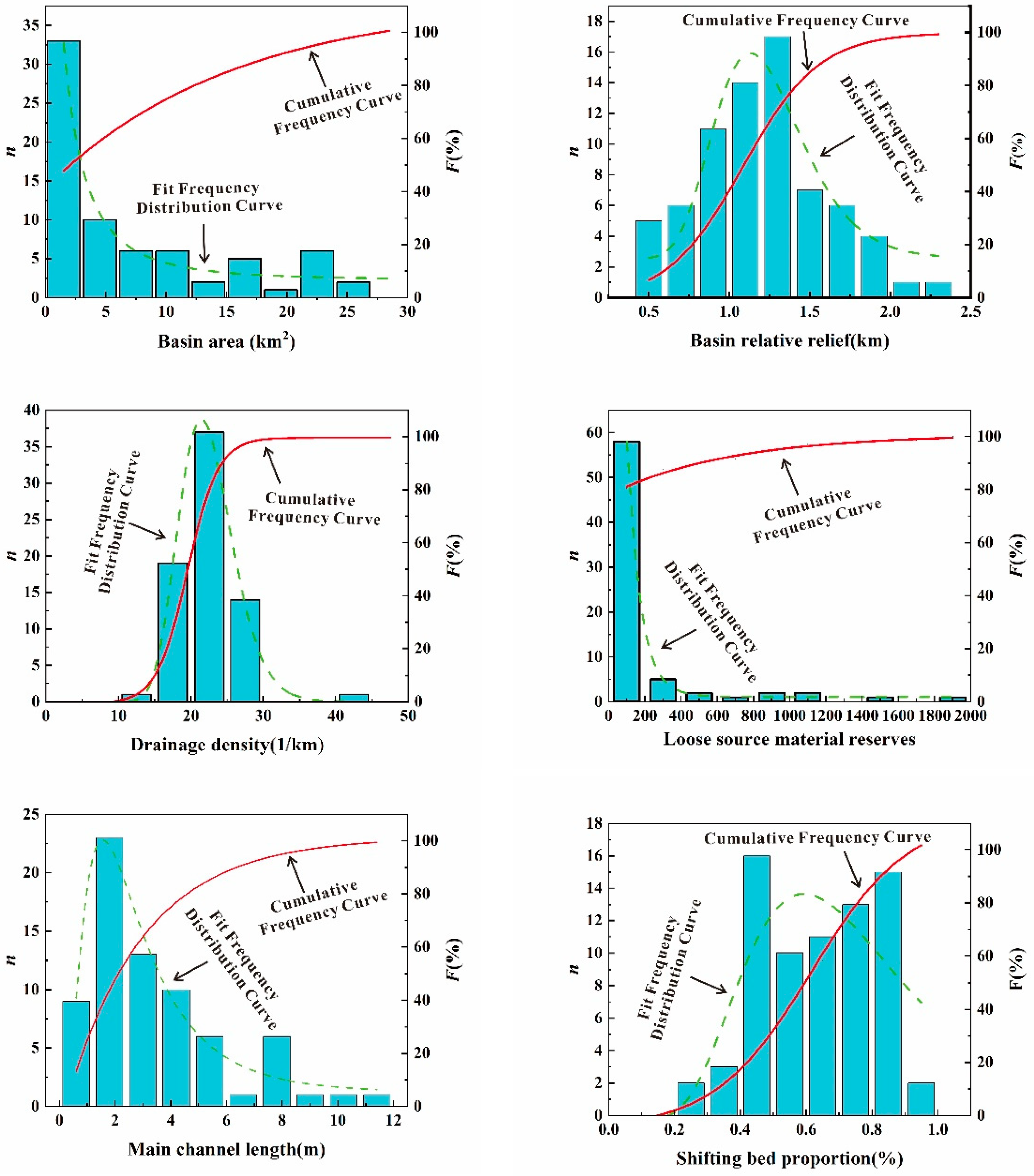
3.2. Parameter Selection
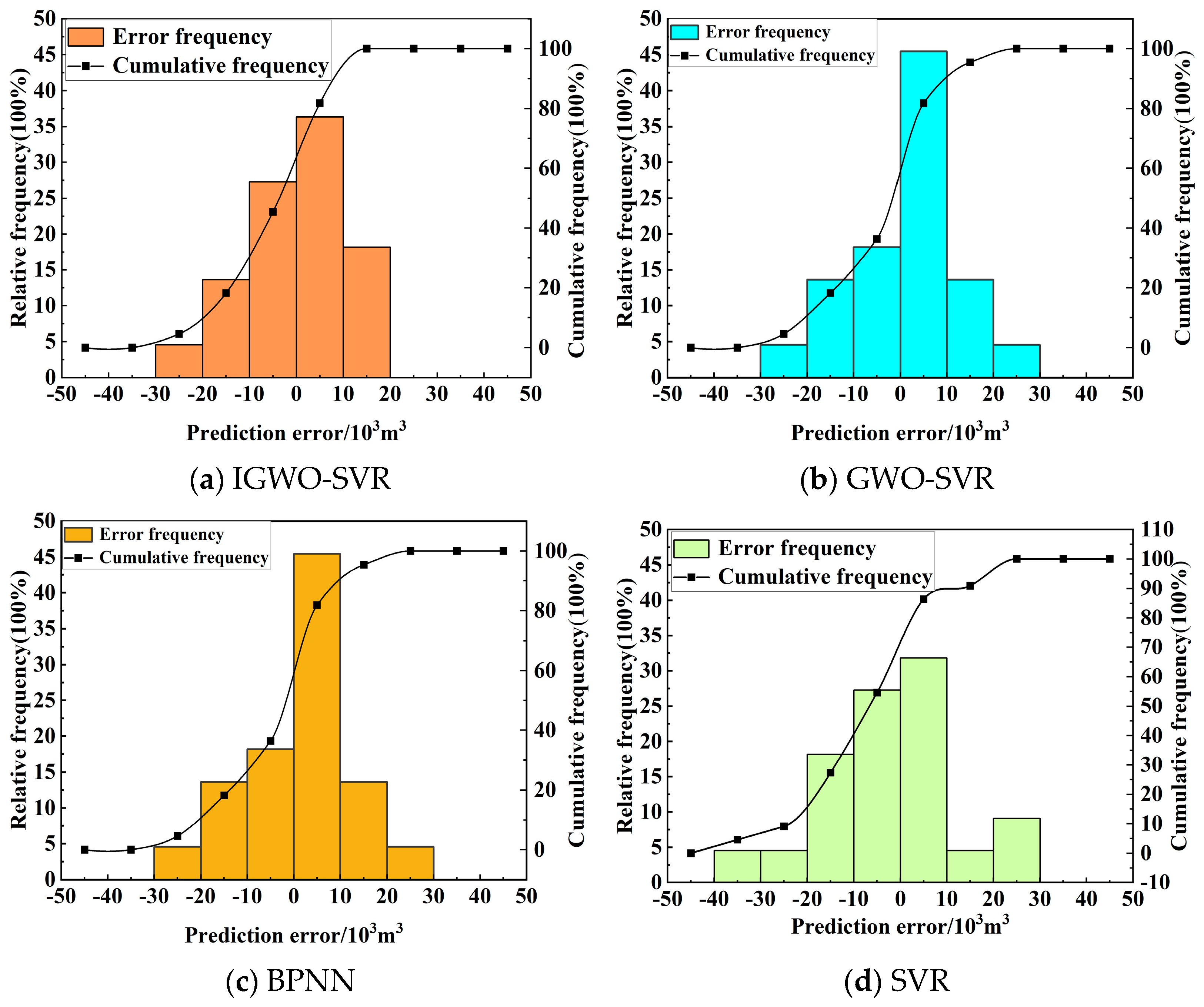
3.3. Data Presentation and Evaluation
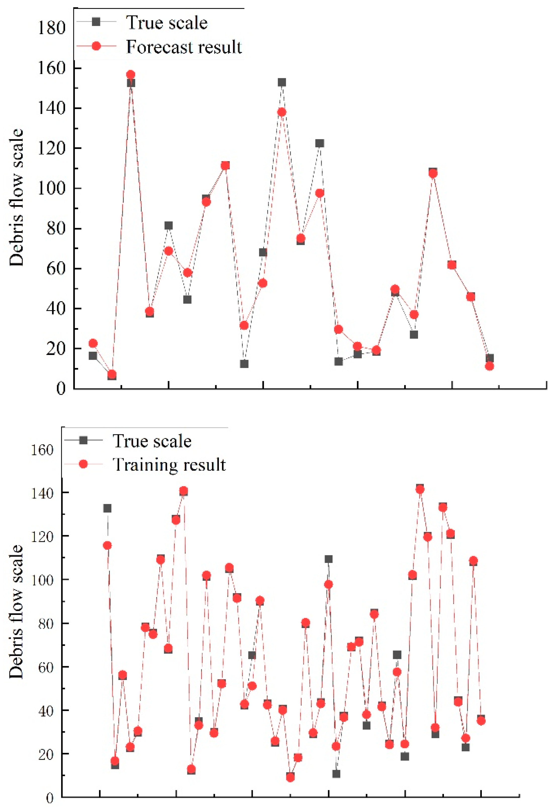
3.4. Forecast of the Debris Flow Scale
3.5. Model Performance Evaluation
3.5.1. Linear Regression Fitting
3.5.2. Power Function Fitting
3.5.3. Comparison with Other Common Optimization Algorithms
4. Discussion
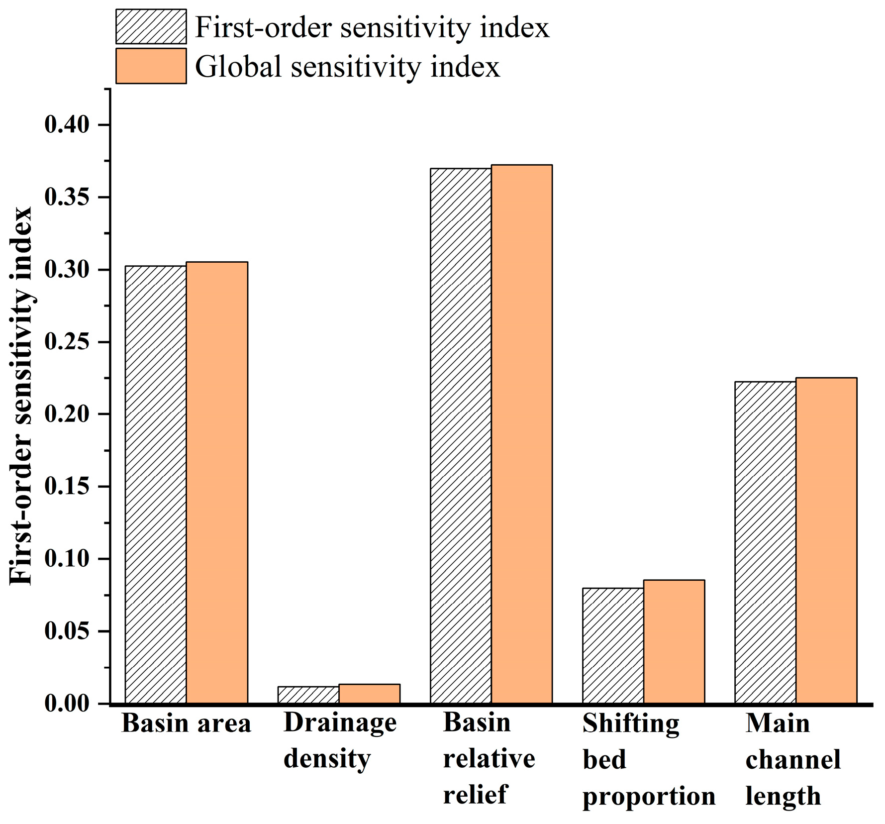
Sobol Method for Sensitivity Analysis
5. Conclusions
- The leading factors of the debris flow scale in Beichuan County are the basin area, the basin relative relief, and the main channel length.
- Aiming to address the shortcomings of support vector machines such as slow convergence speed and ease to fall into local extremes, the improved Grey Wolf Algorithm can improve the prediction speed and accuracy of debris flow scale.
- With regard to the regional characteristics of Beichuan County, since the three influencing factors of basin area, relative height difference and main ditch length have a greater impact on debris flow, when designing the debris flow prevention and control programme, the focus should be on these three factors for consideration.
- The enhanced Grey Wolf Algorithm outlined in this paper lessens the impact of personal opinions and biases on the Debris Flow Scale Prediction process, and the evaluation outcomes give a degree of confidence, thereby offering technological aid for the scientific assessment of Debris Flow danger.
- In the next study, it may be considered to add more data sets using numerical simulation to improve the predictive accuracy of the model. However, increasing the data set will also increase the model run time. Finding a balance between increasing the data set and controlling the model run time is a future direction.
Author Contributions
Funding
Data Availability Statement
Conflicts of Interest
References
- Fuchs, S.; Kaitna, R.; Scheidl, C.; Hübl, J. The application of the risk concept to debris flow hazards. Géoméch. Tunn. 2008, 1, 120–129. [Google Scholar] [CrossRef]
- He, K.; Liu, B.; Hu, X.; Zhou, R.; Xi, C.; Ma, G.; Han, M.; Li, Y.; Luo, G. Rapid characterization of landslide-debris flow chains of geologic hazards using multi-method investigation: Case study of the Tiejiangwan LDC. Rock Mech. Rock Eng. 2022, 55, 5183–5208. [Google Scholar] [CrossRef]
- Trujillo-Vela, M.G.; Ramos-Cañón, A.M.; Escobar-Vargas, J.A.; Galindo-Torres, S.A. An overview of debris-flow mathematical modelling. Earth-Sci. Rev. 2022, 232, 104135. [Google Scholar] [CrossRef]
- de Haas, T.; Densmore, A.L. Debris-flow volume quantile prediction from catchment morphometry. Geology 2019, 47, 791–794. [Google Scholar] [CrossRef]
- Ma, C.; Hu, K.; Tian, M. Comparison of debris-flow volume and activity under different formation conditions. Nat. Hazards 2013, 67, 261–273. [Google Scholar] [CrossRef]
- Gartner, J.E.; Cannon, S.H.; Santi, P.M.; DeWolfe, V.G. Empirical models to predict the volumes of debris flows generated by recently burned basins in the western U.S. Geomorphology 2008, 96, 339–354. [Google Scholar] [CrossRef]
- Chang, C.-W.; Lin, P.-S.; Tsai, C.-L. Estimation of sediment volume of debris flow caused by extreme rainfall in Taiwan. Eng. Geol. 2011, 123, 83–90. [Google Scholar] [CrossRef]
- Arattano, M.; Bertoldi, G.; Cavalli, M.; Comiti, F.; D’Agostino, V.; Theule, J. Comparison of methods and procedures for debris-flow volume estimation. In Engineering Geology for Society and Territory-Volume 3: River Basins, Reservoir Sedimentation and Water Resources; Springer International Publishing: Berlin/Heidelberg, Germany, 2015; pp. 115–119. [Google Scholar]
- Tang, W.; Ding, H.-T.; Chen, N.-S.; Ma, S.-C.; Liu, L.-H.; Wu, K.-L.; Tian, S.-F. Artificial Neural Network-based prediction of glacial debris flows in the ParlungZangbo Basin, southeastern Tibetan Plateau, China. J. Mt. Sci. 2021, 18, 51–67. [Google Scholar] [CrossRef]
- Lee, D.-H.; Cheon, E.; Lim, H.-H.; Choi, S.-K.; Kim, Y.-T.; Lee, S.-R. An artificial neural network model to predict debris-flow volumes caused by extreme rainfall in the central region of South Korea. Eng. Geol. 2021, 281, 105979. [Google Scholar] [CrossRef]
- Huang, F.; Huang, J.; Jiang, S.; Zhou, C. Landslide displacement prediction based on multivariate chaotic model and extreme learning machine. Eng. Geol. 2017, 218, 173–186. [Google Scholar] [CrossRef]
- Xiong, K.; Adhikari, B.R.; Stamatopoulos, C.A.; Zhan, Y.; Wu, S.; Dong, Z.; Di, B. Comparison of different machine learning methods for debris flow susceptibility mapping: A case study in the Sichuan Province, China. Remote Sens. 2020, 12, 295. [Google Scholar] [CrossRef]
- Zhou, X.; Wang, H.; Xu, C.; Peng, L.; Xu, F.; Lian, L.; Deng, G.; Ji, S.; Hu, M.; Zhu, H.; et al. Application of kNN and SVM to predict the prognosis of advanced schistosomiasis. Parasitol. Res. 2022, 121, 2457–2460. [Google Scholar] [CrossRef] [PubMed]
- Pham, V.H.S.; Nguyen, V.N. Cement transport vehicle routing with a hybrid sine cosine optimization algorithm. Adv. Civ. Eng. 2023, 2023, 2728039. [Google Scholar] [CrossRef]
- Shen, D.; Zhang, S.; Ming, W.; He, W.; Zhang, G.; Xie, Z. Development of a new machine vision algorithm to estimate potato’s shape and size based on support vector machine. J. Food Process Eng. 2022, 45, e13974. [Google Scholar] [CrossRef]
- Zhang, J.; Yu, Y.; Zhang, L.; Chen, J.; Wang, X.; Wang, X. Dig information of nanogenerators by machine learning. Nano Energy 2023, 114, 108656. [Google Scholar] [CrossRef]
- Zhou, J.; Huang, S.; Wang, M.; Qiu, Y. Performance evaluation of hybrid GA–SVM and GWO–SVM models to predict earthquake-induced liquefaction potential of soil: A multi-dataset investigation. Eng. Comput. 2021, 38, 4197–4215. [Google Scholar] [CrossRef]
- Bacanin, N.; Antonijevic, M.; Bezdan, T.; Zivkovic, M.; Rashid, T.A. Wireless sensor networks localization by improved whale optimization algorithm. In Proceedings of the 2nd International Conference on Artificial Intelligence: Advances and Applications: ICAIAA 2021, Jaipur, India, 27–28 March 2021; Springer Nature: Singapore, 2022; pp. 769–783. [Google Scholar]
- Mirjalili, S.; Mirjalili, S.M.; Lewis, A. Grey wolf optimizer. Adv. Eng. Softw. 2014, 69, 46–61. [Google Scholar] [CrossRef]
- Liao, K.; Wu, Y.; Miao, F.; Li, L.; Xue, Y. Using a kernel extreme learning machine with grey wolf optimization to predict the displacement of step-like landslide. Bull. Eng. Geol. Environ. 2020, 79, 673–685. [Google Scholar] [CrossRef]
- Mao, M.; Yang, H.; Xu, F.; Ni, P.; Wu, H. Development of geosteering system based on GWO–SVM model. Neural Comput. Appl. 2022, 34, 12479–12490. [Google Scholar] [CrossRef]
- Barthelemy, P.; Bertolotti, J.; Wiersma, D.S. A Lévy flight for light. Nature 2008, 453, 495–498. [Google Scholar] [CrossRef]
- Rong, F.; Dazhi, M.; Dashun, X. Research progress of statistical correlation analysis methods. Math. Model. Its Appl. 2014, 3, 1. (In Chinese) [Google Scholar]
- Wang, X.; Zhao, J.; Li, Q.; Fang, N.; Wang, P.; Ding, L.; Li, S. A hybrid model for prediction in asphalt pavement performance based on support vector machine and grey relation analysis. J. Adv. Transp. 2020, 2020, 7534970. [Google Scholar] [CrossRef]
- Guoqiang, Y.; Maosheng, Z.; Genlong, W.; Liang, P. Comparison and application of support vector machine and BP neural network in predicting average velocity of debris flow. J. Water Resour. 2012, 43, 105–110. (In Chinese) [Google Scholar]
- Ferentinou, M.; Fakir, M. Integrating rock engineering systems device and artificial neural networks to predict stability conditions in an open pit. Eng. Geol. 2018, 246, 293–309. [Google Scholar] [CrossRef]
- Wang, Y.J. Hazard Assessment on Rainstorm Induced Debris Flows in Beichuan County of Wenchuan Earthquake Affected Area; Chengdu University of Technology: Chengdu, China, 2009. (In Chinese) [Google Scholar]
- Markovic, S.; Bryan, J.L.; Ishimtsev, V.; Turakhanov, A.; Rezaee, R.; Cheremisin, A.; Kantzas, A.; Koroteev, D.; Mehta, S.A. Improved oil viscosity characterization by low-field NMR using feature engineering and supervised learning algorithms. Energy Fuels 2020, 34, 13799–13813. [Google Scholar] [CrossRef]
- Chen, P.Y.; Qiao, J.S.; Peng, Z.W.; Xie, K.; Yu, H. Screening of debris flow risk factors and risk evaluation based on rank correlation. Rock Soil Mech. 2013, 34, 1409–1415. (In Chinese) [Google Scholar]
- Ikeya, H.; Mizuyama, T. Flow and Deposit Properties of Debris Flow; Report; Public Works Research Institute: Tsukuba, Japan, 1982; pp. 157–162. [Google Scholar]


| The Basic Data Statistics Table of 72 Debris Flows. | ||||||
|---|---|---|---|---|---|---|
| Samples | Loose Source Material Reserves (103 m3) | Basin Area (km2) | Drainage Density (km−1) | Basin Relative Relief (km) | Shifting Bed Proportion (%) | Main Channel Length (km) |
| Chaimazigou#1 | 0.04 | 2.5 | 8.24 | 1.6 | 0.48 | 2.06 |
| Shuxuegou | 39.04 | 13.9 | 2.90 | 1.4 | 0.50 | 4.03 |
| Yingtaogou#1 | 43.65 | 10.3 | 3.78 | 1.4 | 0.72 | 3.89 |
| Miaobagou | 728.20 | 7.8 | 5.26 | 1.46 | 0.85 | 4.10 |
| Jinlongcun | 79.50 | 4.5 | 7.44 | 0.98 | 0.64 | 3.35 |
| Hualingou | 385.95 | 12.2 | 4.82 | 1.36 | 0.85 | 5.88 |
| Wangjiashangou | 104.50 | 1.8 | 7.67 | 1.04 | 0.86 | 1.38 |
| Xinzhigou#1 | 240.45 | 10 | 5.39 | 1.56 | 0.76 | 5.39 |
| Chenjiabaogou | 50.20 | 1.9 | 7.16 | 1.1 | 0.48 | 1.36 |
| Pijialianggou | 2.40 | 2.4 | 7.42 | 1.14 | 0.23 | 1.78 |
| Xishanpogou | 1500 | 1.6 | 20.75 | 1.12 | 0.61 | 3.32 |
| Renjiapinggou | 242 | 0.5 | 14.6 | 0.46 | 0.84 | 0.73 |
| Mofanggou | 160.70 | 0.8 | 13.63 | 0.66 | 0.72 | 1.09 |
| Miaobagou | 6.60 | 7.5 | 3.81 | 1.38 | 0.39 | 2.86 |
| Piankoxianggou#2 | 4.80 | 4.6 | 4.33 | 0.86 | 0.54 | 1.99 |
| Xinzhigou#2 | 73.20 | 21.8 | 3.59 | 2.04 | 0.42 | 7.82 |
| Honglingou | 2.85 | 5.7 | 5.35 | 1.92 | 0.37 | 3.05 |
| Chaimazigou#2 | 14.70 | 6.8 | 3.75 | 1.8 | 0.40 | 2.55 |
| Qinglingou | 109.30 | 23.2 | 3.23 | 2.3 | 0.61 | 7.49 |
| Baishuihegou | 35 | 10.6 | 4.01 | 1.68 | 0.47 | 4.25 |
| Piankoxianggou#3 | 160.34 | 16 | 3.68125 | 1.04 | 0.51 | 5.89 |
| Subaohegou | 60 | 3.5 | 6.43 | 1.24 | 0.65 | 2.25 |
| Shuligou | 70.60 | 0.7 | 20.43 | 0.96 | 0.61 | 1.43 |
| Xinigou | 40.53 | 0.7 | 19.43 | 1 | 0.81 | 1.36 |
| Tianbaigou | 163.32 | 18.7 | 3.16 | 1.68 | 0.76 | 5.91 |
| Piankoxianggou | 0.89 | 0.9 | 15.11 | 0.72 | 0.43 | 1.36 |
| Lijiawangou | 60 | 1.2 | 12.08 | 0.86 | 0.41 | 1.45 |
| Kaipingzhigou | 26.20 | 1 | 13.20 | 0.6 | 0.62 | 1.32 |
| Yuxuegou | 1016.40 | 0.8 | 14.38 | 0.88 | 0.86 | 1.15 |
| Xiatongbaogou | 1967.90 | 15.7 | 3.80 | 1.22 | 0.84 | 5.97 |
| Sibapinggou | 378.24 | 21.4 | 3.47 | 1.5 | 0.76 | 7.42 |
| Zhibeigou | 199 | 8.7 | 3.25 | 1.36 | 0.60 | 2.83 |
| Yangliucun | 101.63 | 9.9 | 4.64 | 1.7 | 0.58 | 4.59 |
| Yanghuziwangou | 40.20 | 1.2 | 12.08 | 0.82 | 0.81 | 1.45 |
| Zhifanggou | 74 | 1.1 | 9.55 | 0.75 | 0.69 | 1.05 |
| Yingtaogou#2 | 119.30 | 17.6 | 4.33 | 1.66 | 0.56 | 7.62 |
| Sunjiagou | 15.55 | 2.7 | 10.70 | 1.22 | 0.45 | 2.89 |
| Chayuanlianggou | 54 | 2.6 | 12.04 | 1.26 | 0.41 | 3.13 |
| Hanjiashangou | 67.44 | 0.8 | 15.25 | 0.82 | 0.82 | 1.22 |
| Baiguoshugou | 107.30 | 0.6 | 16.50 | 0.67 | 0.73 | 0.99 |
| Weigou | 33.54 | 2.2 | 9.50 | 0.74 | 0.57 | 2.09 |
| Weigou#2 | 106.50 | 0.3 | 22.00 | 0.52 | 0.76 | 0.66 |
| Madiwangou | 3.36 | 0.7 | 29.86 | 0.55 | 0.47 | 2.09 |
| Huangjiawangou | 4.13 | 2.8 | 8.39 | 1 | 0.47 | 2.35 |
| Jingzhuyuangou | 51.80 | 1.1 | 9.00 | 0.59 | 0.46 | 0.99 |
| Jiangjiagou | 12.14 | 0.5 | 23.00 | 0.92 | 0.52 | 1.15 |
| Maoershi | 10.80 | 1.4 | 7.57 | 0.98 | 0.47 | 1.06 |
| Subaogou | 507 | 1.1 | 10.45 | 0.58 | 0.79 | 1.15 |
| Liujiagou | 120.08 | 1.8 | 7.50 | 1.04 | 0.89 | 1.35 |
| Daokaimengou | 15.98 | 3.1 | 8.19 | 0.84 | 0.51 | 2.54 |
| Qingtangwangou | 30 | 3.5 | 5.14 | 0.82 | 0.75 | 1.80 |
| Huangtulianggou | 114 | 24.6 | 3.29 | 1.22 | 0.64 | 8.10 |
| Guanmenzigou | 14.26 | 2.8 | 5.57 | 1.12 | 0.70 | 1.56 |
| Shupinggou | 33 | 4.1 | 8.88 | 1.09 | 0.46 | 3.64 |
| Dengjiacungou | 900.03 | 22.2 | 5.12 | 1.7 | 0.44 | 11.36 |
| Qushanzhenggou | 210 | 3.6 | 8.67 | 1.2 | 0.96 | 3.12 |
| Guzhubagou | 1000.10 | 7 | 5.74 | 1.22 | 0.87 | 4.02 |
| Wangjiayangou | 485 | 2.5 | 7.88 | 1 | 0.81 | 1.97 |
| Chenjiabagou | 931.24 | 23.1 | 4.28 | 1.2 | 0.66 | 9.88 |
| Tudilianggou | 12.21 | 4 | 6.40 | 1.03 | 0.53 | 2.56 |
| Tudimiaogou | 34.08 | 16 | 3.69 | 1.28 | 0.39 | 5.91 |
| Guaitangou | 0.08 | 11.7 | 4.05 | 1.08 | 0.21 | 4.74 |
| Dapingdigou | 16.80 | 5.4 | 5.59 | 1.46 | 0.40 | 3.02 |
| Xiatongbaogou | 98.50 | 22.7 | 3.37 | 1.86 | 0.76 | 7.66 |
| Chanzipinggou | 67.20 | 2.5 | 5.28 | 1.02 | 0.83 | 1.32 |
| Shangyantaigou | 17.50 | 1.5 | 11.67 | 1.24 | 0.9 | 1.75 |
| Shuangyigou | 93.30 | 2.8 | 9.82 | 1.3 | 0.78 | 2.75 |
| Shilonggou | 50.80 | 7.3 | 5.36 | 1.2 | 0.84 | 3.91 |
| Yangjiawangou | 135.57 | 26.4 | 3.20 | 1.8 | 0.67 | 8.46 |
| Zhaojiawangou | 14.66 | 2.8 | 8.18 | 1.34 | 0.82 | 2.29 |
| Dongxigou | 8.95 | 10.9 | 3.78 | 1.5 | 0.57 | 4.12 |
| Maliuwangou | 97.82 | 17.1 | 3.76 | 1.28 | 0.70 | 6.43 |
| Data Type | Loose Source Material Reserves (103 m3) | Basin Area (km2) | Drainage Density (km−1) | Basin Relative Relief (km) | Shifting Bed Proportion (%) | Main Channel Length (km) | Debris Flow Scale |
|---|---|---|---|---|---|---|---|
| minimum value | 0.04 | 0.3 | 10.68 | 0.46 | 0.21 | 0.66 | 6.3 |
| maximum value | 1966.9 | 26.4 | 44.06 | 2.3 | 0.96 | 11.36 | 152.83 |
| average value | 195.93 | 7.10 | 22.18 | 1.18 | 0.63 | 3.40 | 62.85 |
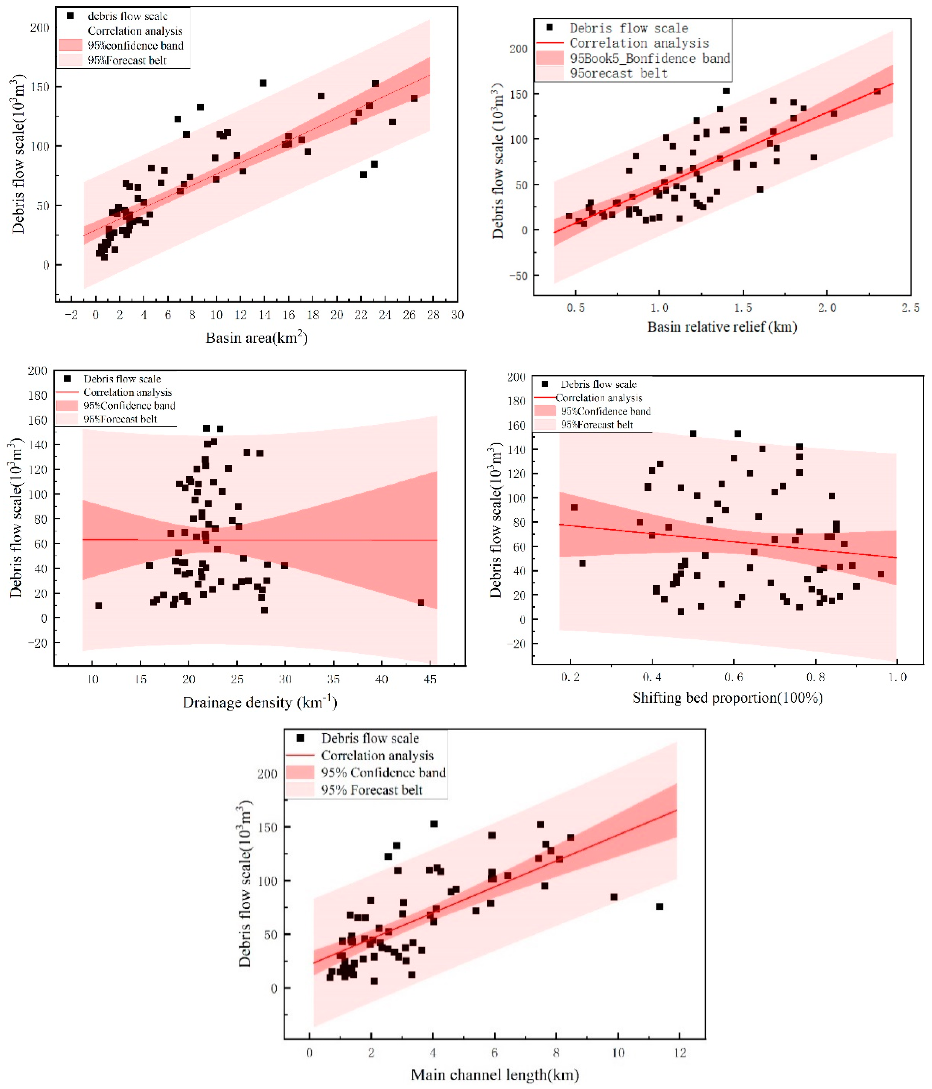
| Correlation Analysis | |
|---|---|
| Correlation Factor | Debris Flow Scale (103 m3) |
| Basin area/km2 | 0.920 ** |
| Drainage density/1/km | 0.136 |
| Basin relative relief/km | 0.778 ** |
| Shifting bed proportion/% | −0.154 |
| Main channel length/km | 0.766 ** |
| Linear Regression Analysis Results | |||||||||
|---|---|---|---|---|---|---|---|---|---|
| Unstandardized Coefficients | Standardized Coefficient | t | p | VIF | R2 | Adjust R2 | F | ||
| B | Standard Error | Beta | |||||||
| constant | 14.818 | 7.171 | - | 2.066 | 0.044 * | - | 0.904 | 0.898 | F (3,46) = 144.282 p = 0.000 |
| Basin area | 10.334 | 1.035 | 1.538 | 9.988 | 0.000 ** | 11.354 | |||
| Basin relative relief | 39.329 | 7.251 | 0.385 | 5.424 | 0.000 ** | 2.414 | |||
| Main channel length | −21.377 | 3.322 | −0.993 | −6.436 | 0.000 ** | 11.396 | |||
| Prediction Error Analysis of Different Prediction Models | |||
|---|---|---|---|
| Name | RMSE | MAE | R2 |
| IGOW-SVR | 7.75 | 7.0 | 0.95 |
| GOW-SVR | 7.80 | 7.6 | 0.94 |
| SVR | 10.99 | 8.79 | 0.92 |
| BPNN | 13.70 | 14.47 | 0.83 |
| Prediction Model Consumption Time Comparison | ||||
|---|---|---|---|---|
| SVR | BPNN | GWO-SVR | IGWO-SVR | SVR |
| Time/s | 3.6226 | 5.4500 | 2.3141 | 1.7876 |
Disclaimer/Publisher’s Note: The statements, opinions and data contained in all publications are solely those of the individual author(s) and contributor(s) and not of MDPI and/or the editor(s). MDPI and/or the editor(s) disclaim responsibility for any injury to people or property resulting from any ideas, methods, instructions or products referred to in the content. |
© 2023 by the authors. Licensee MDPI, Basel, Switzerland. This article is an open access article distributed under the terms and conditions of the Creative Commons Attribution (CC BY) license (https://creativecommons.org/licenses/by/4.0/).
Share and Cite
Li, L.; Zhang, Z.; Zhao, D.; Qiang, Y.; Ni, B.; Wu, H.; Hu, S.; Lin, H. Debris Flow Scale Prediction Based on Correlation Analysis and Improved Support Vector Machine. Water 2023, 15, 4161. https://doi.org/10.3390/w15234161
Li L, Zhang Z, Zhao D, Qiang Y, Ni B, Wu H, Hu S, Lin H. Debris Flow Scale Prediction Based on Correlation Analysis and Improved Support Vector Machine. Water. 2023; 15(23):4161. https://doi.org/10.3390/w15234161
Chicago/Turabian StyleLi, Li, Zhongxu Zhang, Dongsheng Zhao, Yue Qiang, Bo Ni, Hengbin Wu, Shengchao Hu, and Hanjie Lin. 2023. "Debris Flow Scale Prediction Based on Correlation Analysis and Improved Support Vector Machine" Water 15, no. 23: 4161. https://doi.org/10.3390/w15234161