
Assessing the Impact of Human Activities and Climate Change Effects on Groundwater Quantity and Quality: A Case Study of the Western Varamin Plain, Iran
Abstract
:1. Introduction
2. Materials and Methods
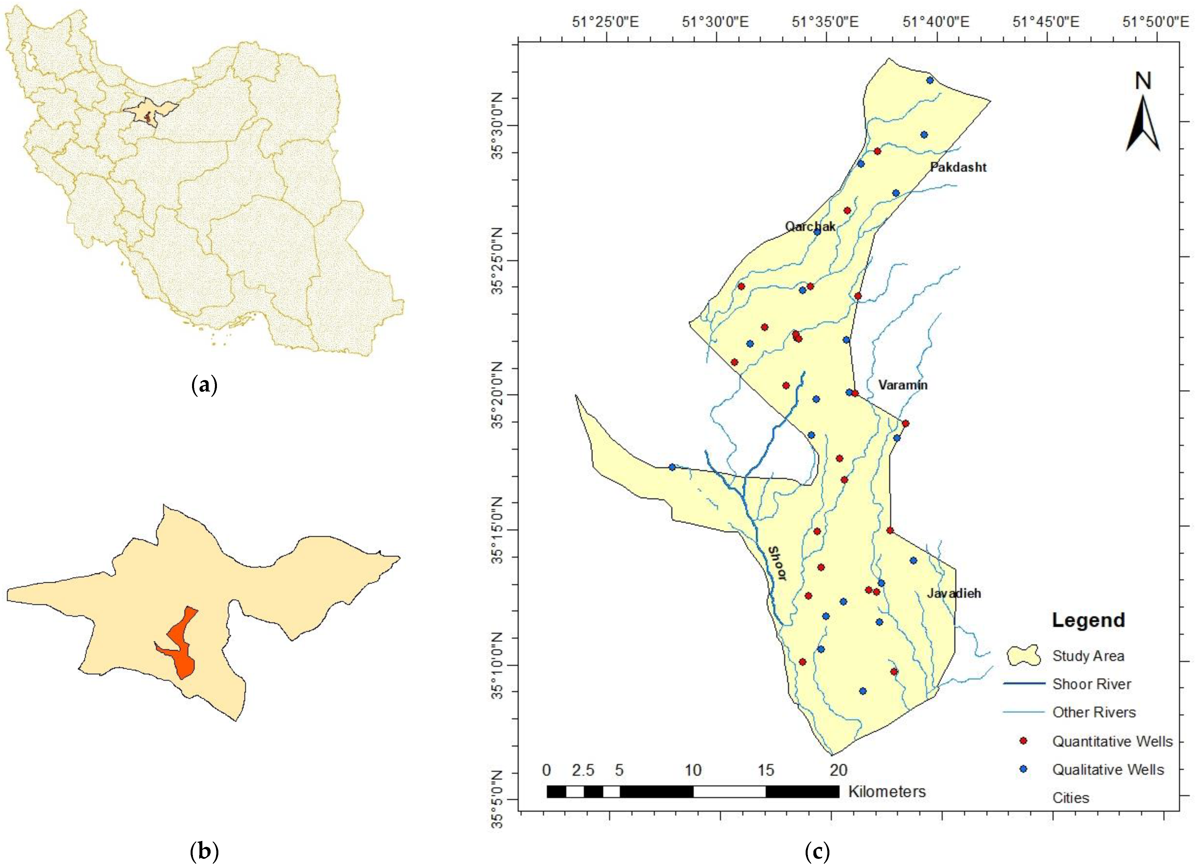
2.1. Study Area
2.2. General Framework of Modeling
2.3. Models Used in Quantitative and Qualitative Simulation
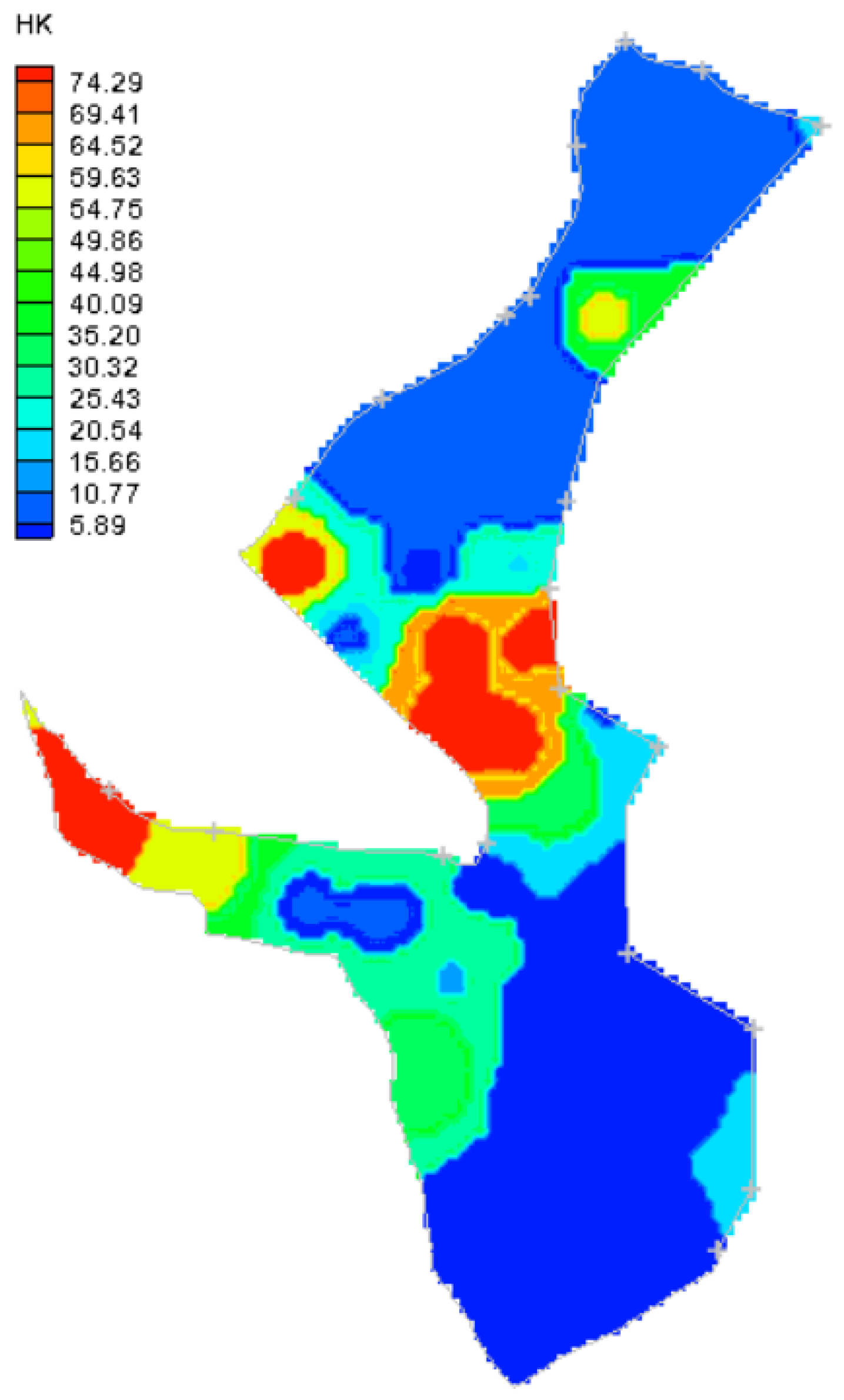
2.4. Primary Information of Groundwater Flow Modeling
2.5. Primary Information of Transport Modeling
2.6. Climate Change Scenarios and Downscaling
2.7. Determination of ET0, ETC, and IWN
3. Result
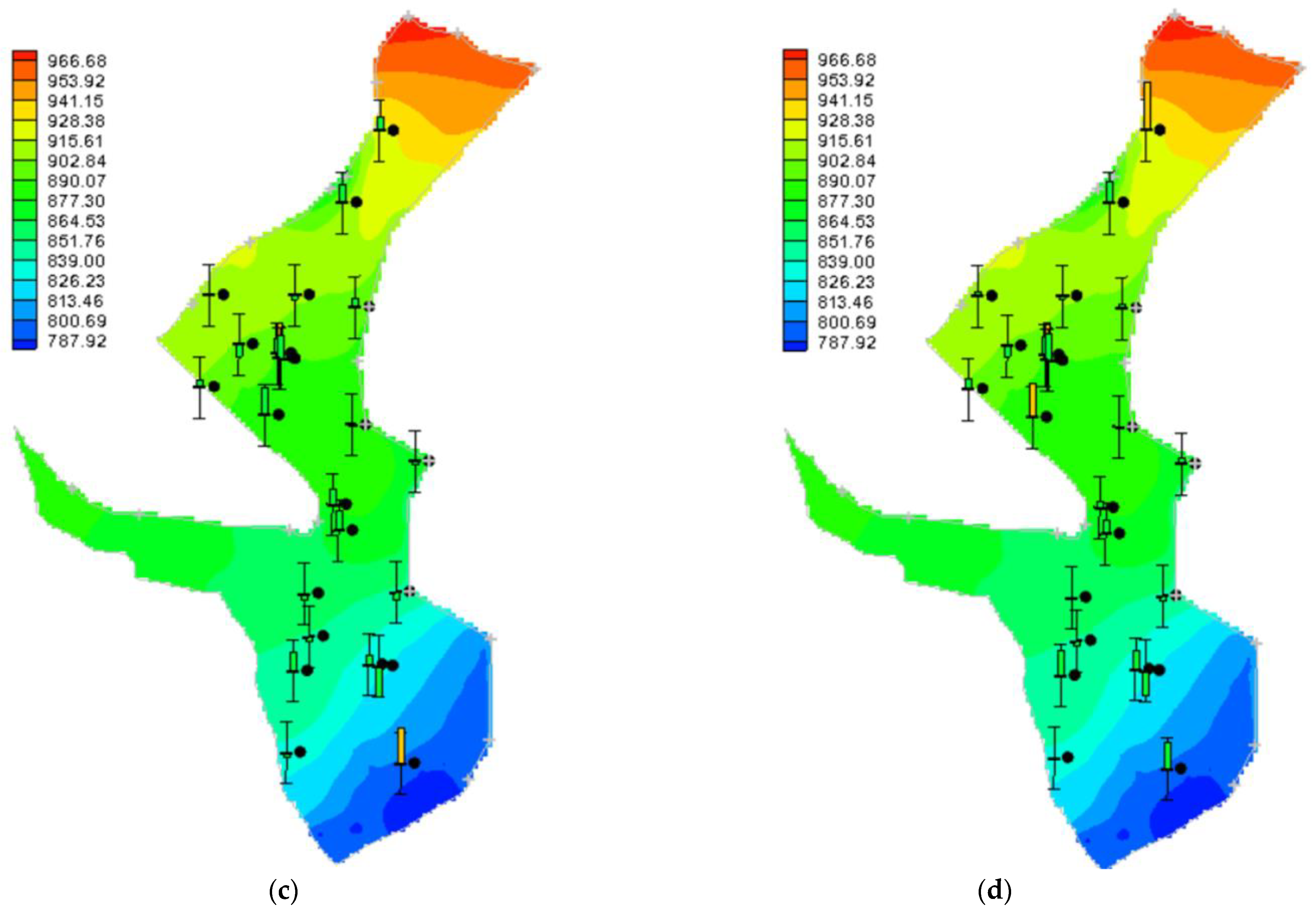
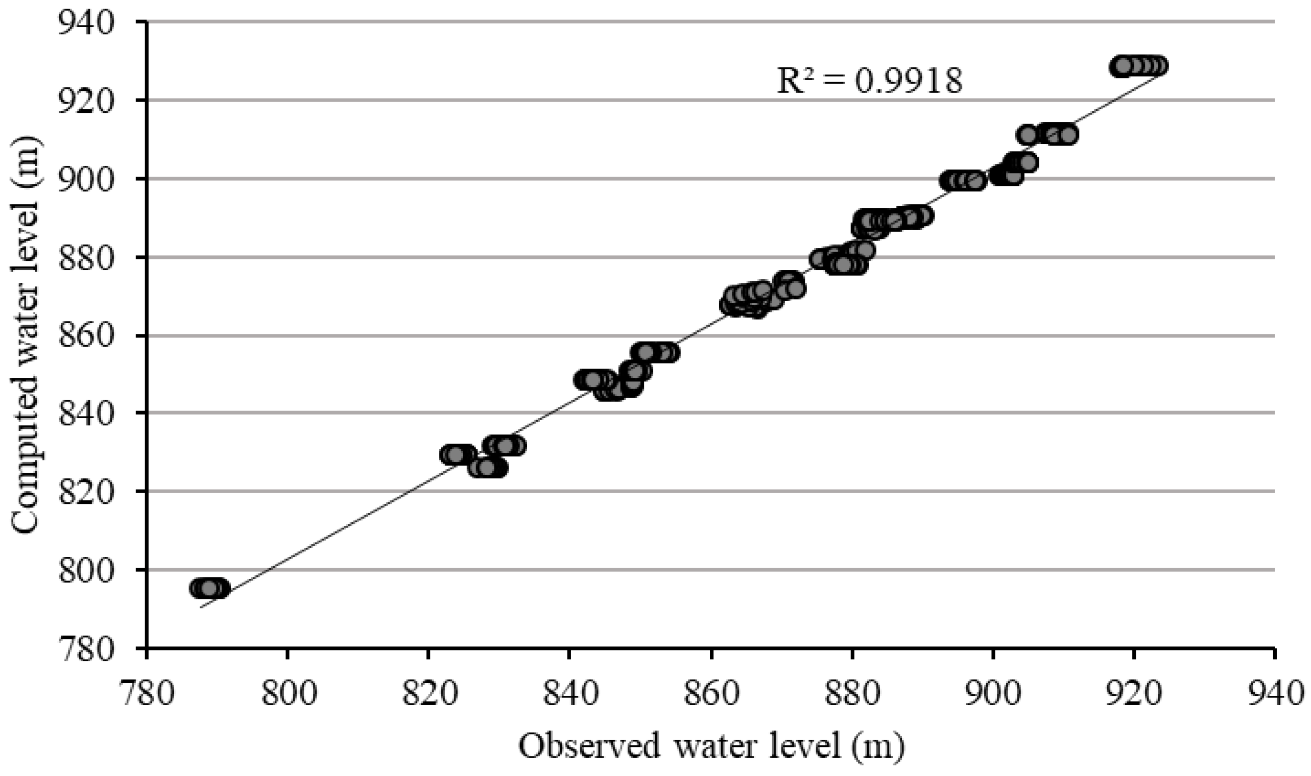
3.1. MODFLOW Calibration and Validation Results
3.2. MT3D Calibration and Validation Results
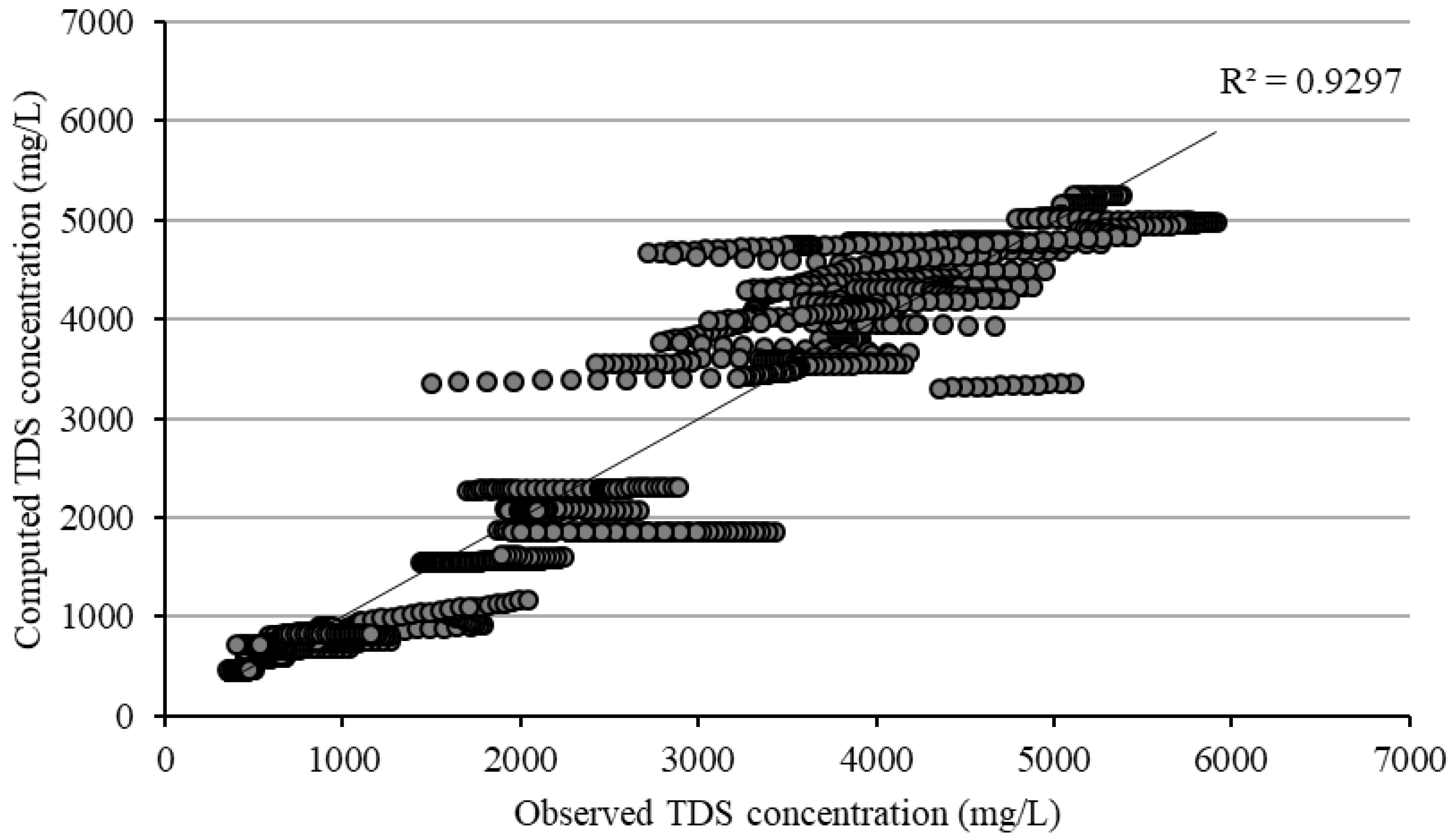
3.2.1. TDS
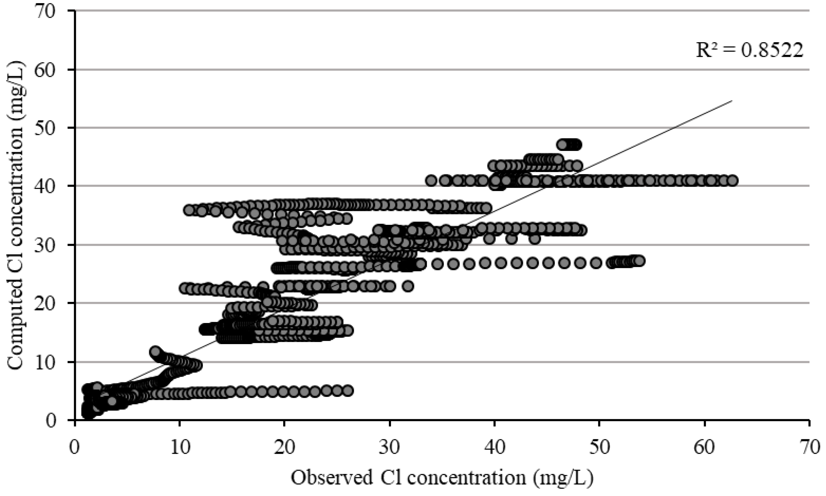
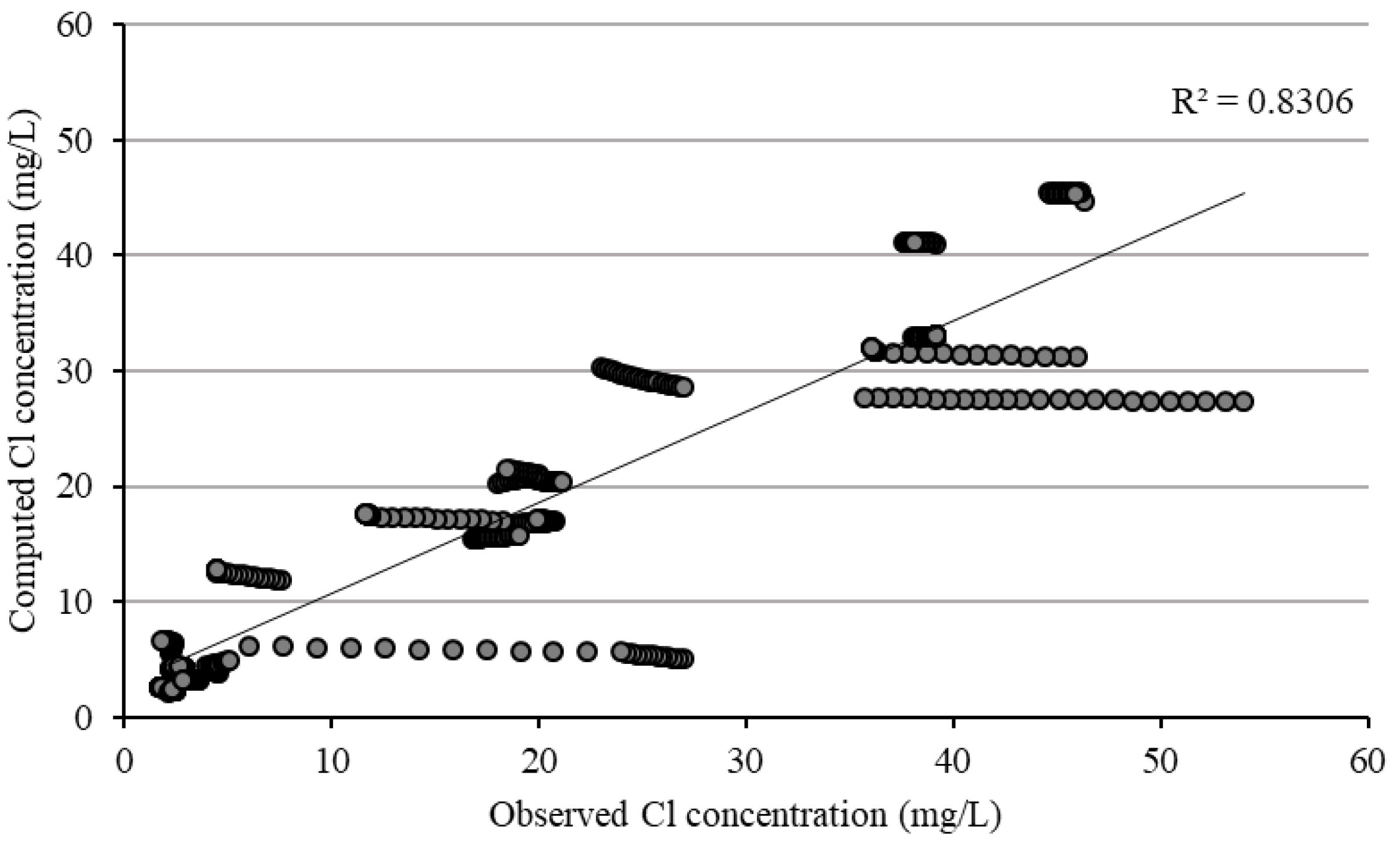
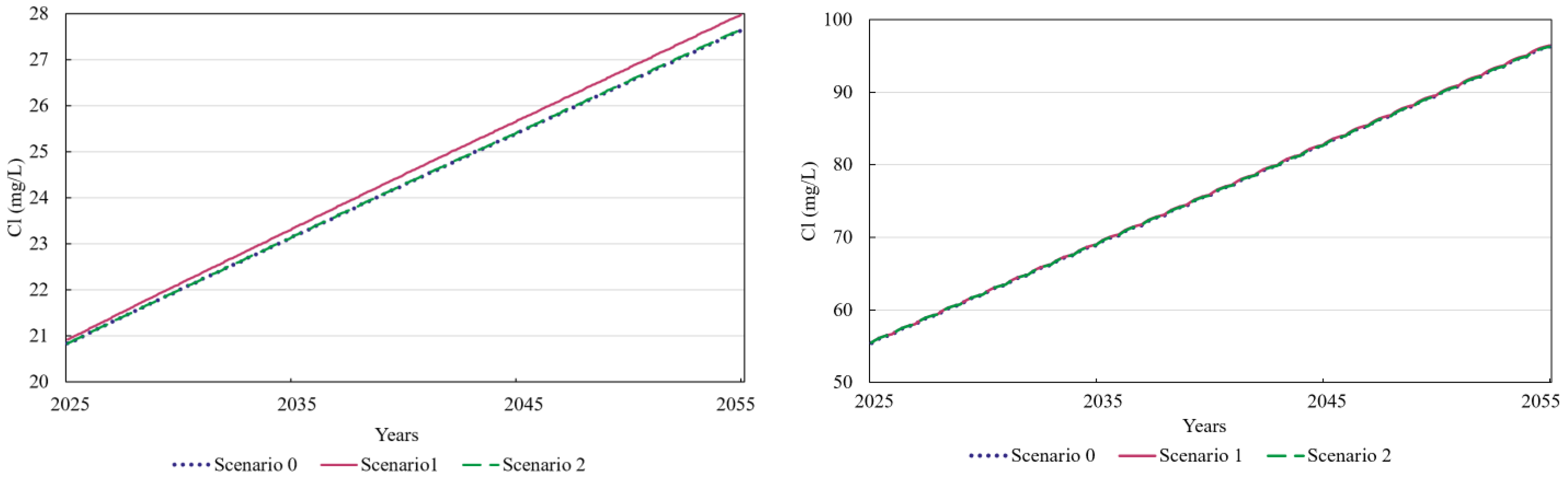
3.2.2. Chloride
3.2.3. Sodium Ion
3.3. SDSM Calibration, Validation, and Prediction Results
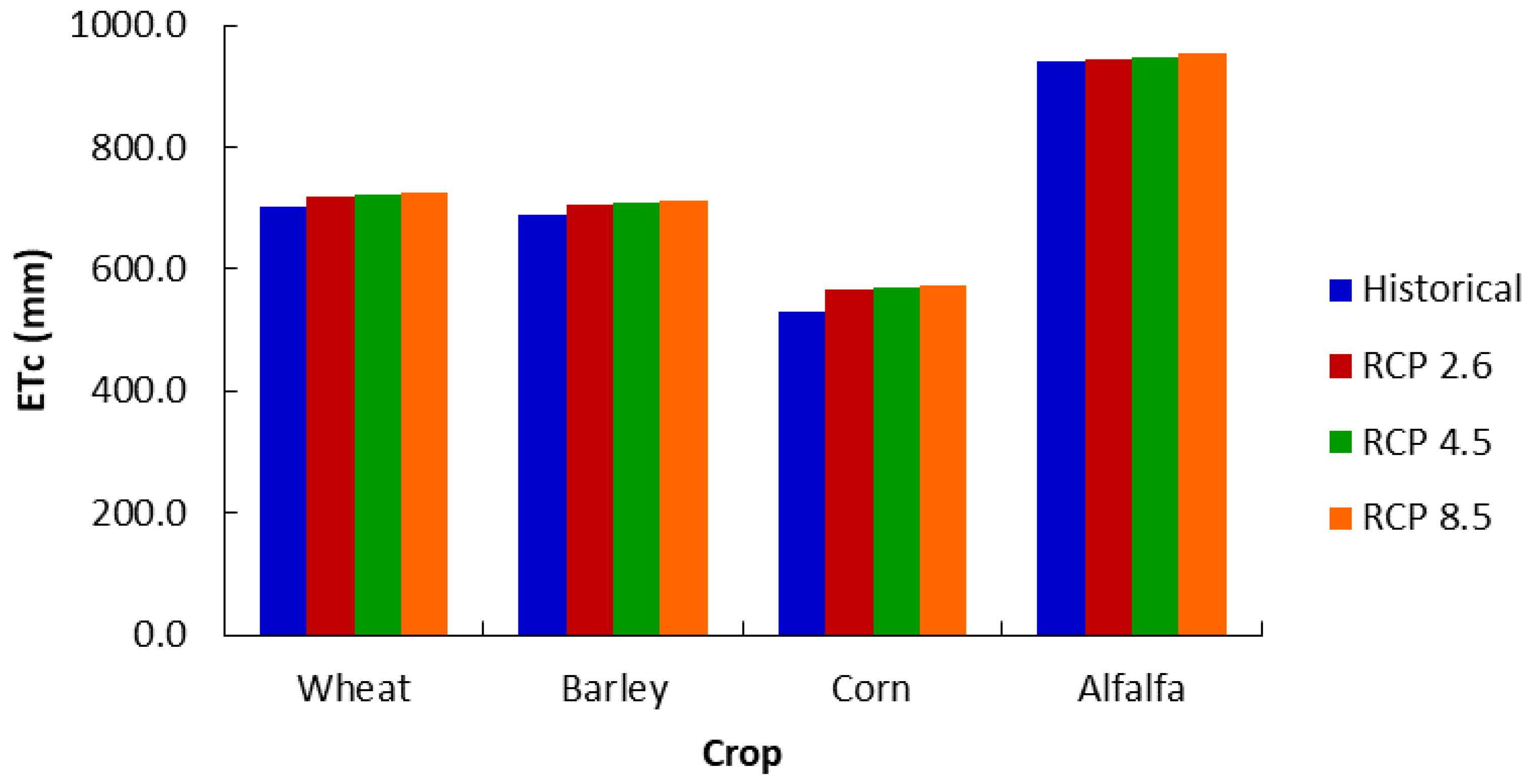
3.4. Climate Change Effect on ET0, ETC, and IWN
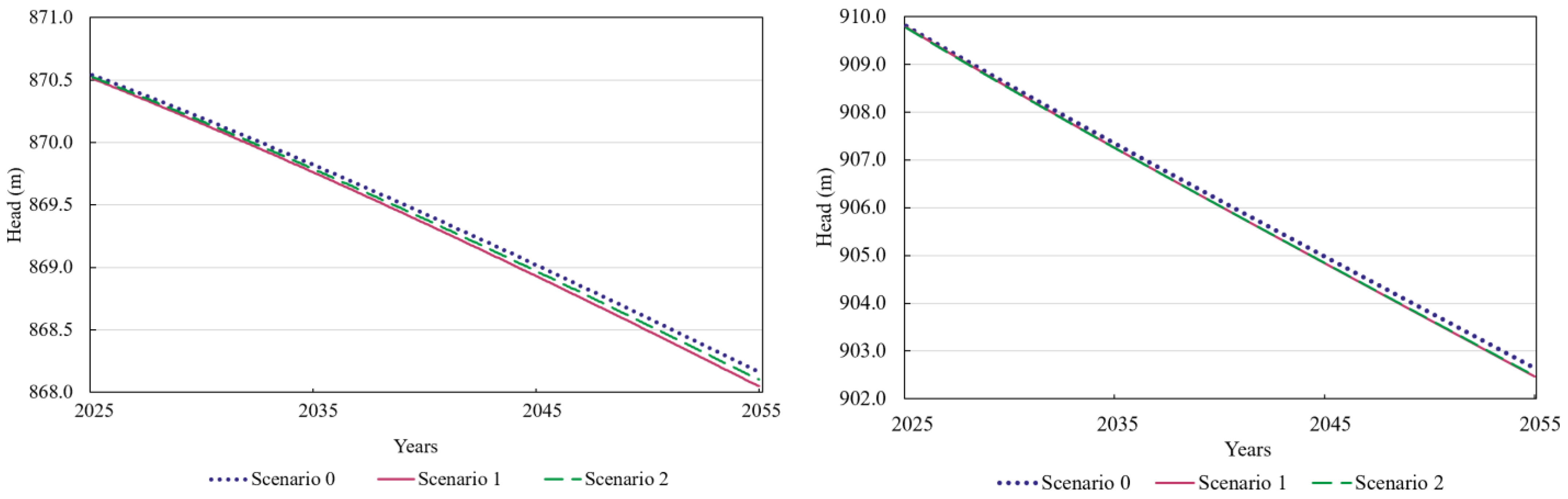
3.5. Predicting the Aquifer’s Status in the Future
3.5.1. Scenario 0: Continuing the Existing Conditions
3.5.2. Scenario 1: Increase in the Extraction from Pumping Wells (25%)
3.5.3. Scenario 2: Climate Changes
3.5.4. Scenario 3: Increase in the Incoming Effluent (TDS) to the Shoor River (50%)
4. Discussion
5. Conclusions
Author Contributions
Funding
Data Availability Statement
Conflicts of Interest
References
- Fetter, C.W. Applied Hydrogeology, 4th ed.; PrenticeHall: Englewood Cliffs, NJ, USA, 2001; pp. 1–20. [Google Scholar]
- Döll, P.; Hoffmann-Dobrev, H.; Portmann, F.T.; Siebert, S.; Eicker, A.; Rodell, M.; Strassberg, G.; Scanlon, B.R. Impact of water withdrawals from groundwater and surface water on continental water storage variations. J. Geodyn. 2012, 59, 143–156. [Google Scholar] [CrossRef]
- Hall, N.D.; Stuntz, B.B.; Abrams, R.H. Climate change and freshwater resources. Nat. Resour. Environ. 2008, 22, 30–35. [Google Scholar]
- Li, R.; Merchant, J.W. Modeling vulnerability of groundwater to pollution under future scenarios of climate change and biofuels-related land use change: A case study in North Dakota, USA. Sci. Total Environ. J. 2013, 447, 32–45. [Google Scholar] [CrossRef]
- Kumar, C.P. Climate change and its impact on groundwater resources. Int. J. Eng. Sci. 2012, 1, 43–60. [Google Scholar]
- Earman, S.; Dettinger, M. Potential impacts of climate change on groundwater resources—A global review. J. Water Clim. Chang. 2011, 2, 213–229. [Google Scholar] [CrossRef]
- Dragoni, W.; Sukhija, B.S. Climate change and groundwater: A short review. J. Geol. Soc. 2008, 288, 1–12. [Google Scholar] [CrossRef]
- Taylor, R.G.; Scanlon, B.; Döll, P.; Rodell, M.; Van Beek, R.; Wada, Y.; Longuevergne, L.; Leblanc, M.; Famiglietti, J.S.; Edmunds, M.; et al. Ground water and climate change. Nat. Clim. Chang. 2013, 3, 322–329. [Google Scholar] [CrossRef]
- Amanambu, A.C.; Obarein, O.A.; Mossa, J.; Li, L.; Ayeni, S.S.; Balogun, O.; Oyebamiji, A.; Ochege, F.U. Groundwater system and climate change: Present status and future considerations. J. Hydrol. 2020, 589, 125163. [Google Scholar] [CrossRef]
- Pachauri, R.K.; Reisinger, A. Climate Change 2007: Synthesis Report. Contribution of Working Groups I, II and III to the Fourth Assessment Report of the Intergovernmental Panel on Climate Change; IPCC: Geneva, Switzerland, 2007; p. 104. [Google Scholar]
- Zhou, T.; Wu, P.; Sun, S.; Li, X.; Wang, Y.; Luan, X. Impact of future climate change on regional crop water requirement—A case study of Hetao Irrigation District, China. Water 2017, 9, 429. [Google Scholar] [CrossRef]
- Goodarzi, M.; Abedi-Koupai, J.; Heidarpour, M. Investigating impacts of climate change on irrigation water demands and its resulting consequences on groundwater using CMIP5 models. Groundwater 2019, 57, 259–268. [Google Scholar] [CrossRef]
- Elnashar, W.; Elyamany, A. Managing risks of climate change on irrigation water in arid regions. Water Resour. Manag. 2023, 37, 2429–2446. [Google Scholar] [CrossRef]
- Green, T.R.; Taniguchi, M.; Kooi, H.; Gurdak, J.J.; Allen, D.M.; Hiscock, K.M.; Treidel, H.; Aureli, A. Beneath the surface of global change: Impacts of climate change on groundwater. J. Hydrol. 2011, 405, 532–560. [Google Scholar] [CrossRef]
- Allen, D.M.; Mackie, D.C.; Wei, M.J.H.J. Groundwater and climate change: A sensitivity analysis for the Grand Forks aquifer, southern British Columbia, Canada. Hydrogeol. J. 2004, 12, 270–290. [Google Scholar] [CrossRef]
- Allen, D.M.; Cannon, A.J.; Toews, M.W.; Scibek, J. Variability in simulated recharge using different GCMs. Water Resour. Res. 2010, 46, 1–18. [Google Scholar] [CrossRef]
- Meixner, T.; Manning, A.H.; Stonestrom, D.A.; Allen, D.M.; Ajami, H.; Blasch, K.W.; Brookfield, A.E.; Castro, C.L.; Clark, J.F.; Gochis, D.J.; et al. Implications of projected climate change for groundwater recharge in the western United States. J. Hydrol. 2016, 534, 124–138. [Google Scholar] [CrossRef]
- Hughes, A.; Mansour, M.; Ward, R.; Kieboom, N.; Allen, S.; Seccombe, D.; Charlton, M.; Prudhomme, C. The impact of climate change on groundwater recharge: National-scale assessment for the British mainland. J. Hydrol. 2021, 598, 126336. [Google Scholar] [CrossRef]
- Pachauri, R.K.; Allen, M.R.; Barros, V.R.; Broome, J.; Cramer, W.; Christ, R.; Church, J.A.; Clarke, L.; Dahe, Q.; Dasgupta, P.; et al. Climate Change 2014: Synthesis Report. Contribution of Working Groups I, II and III to the Fifth Assessment Report of the Intergovernmental Panel on Climate Change; IPCC: Geneva, Switzerland, 2014; p. 151. [Google Scholar]
- Swart, N.C.; Cole, J.N.; Kharin, V.V.; Lazare, M.; Scinocca, J.F.; Gillett, N.P.; Anstey, J.; Arora, V.; Christian, J.R.; Hanna, S.; et al. The Canadian earth system model version 5 (CanESM5. 0.3). Geosci. Model Dev. 2019, 12, 4823–4873. [Google Scholar] [CrossRef]
- Arora, V.K.; Scinocca, J.F.; Boer, G.J.; Christian, J.R.; Denman, K.L.; Flato, G.M.; Kharin, V.V.; Lee, W.G.; Merryfield, W.J. Carbon emission limits required to satisfy future representative concentration pathways of greenhouse gases. Geophys. Res. Lett. 2011, 38, 1–6. [Google Scholar] [CrossRef]
- Venkataraman, K.; Tummuri, S.; Medina, A.; Perry, J. 21st century drought outlook for major climate divisions of Texas based on CMIP5 multimodel ensemble: Implications for water resource management. J. Hydrol. 2016, 534, 300–316. [Google Scholar] [CrossRef]
- Chylek, P.; Li, J.; Dubey, M.K.; Wang, M.; Lesins, G.J.A.C. Observed and model simulated 20th century Arctic temperature variability: Canadian earth system model CanESM2. Atmos. Chem. Phys. Discuss 2011, 11, 22893–22907. [Google Scholar]
- Hua, W.; Chen, H.; Sun, S.; Zhou, L. Assessing climatic impacts of future land use and land cover change projected with the CanESM2 model. Int. J. Climatol. 2015, 35, 3661–3675. [Google Scholar] [CrossRef]
- Hassan, W.H.; Nile, B.K. Climate change and predicting future temperature in Iraq using CanESM2 and HadCM3 modeling. Model. Earth Syst. Environ. 2021, 7, 737–748. [Google Scholar] [CrossRef]
- Wilby, R.L.; Charles, S.P.; Zorita, E.; Timbal, B.; Whetton, P.; Mearns, L.O. Guidelines for use of climate scenarios developed from statistical downscaling methods. In Supporting Material of the Intergovernmental Panel on Climate Change, Available from the DDC of IPCC TGCIA; IPCC: Geneva, Switzerland, 2004. [Google Scholar]
- Wilby, R.L.; Dawson, C.W.; Barrow, E.M. SDSM—A decision support tool for the assessment of regional climate change impacts. Environ. Model. Softw. 2002, 17, 45–157. [Google Scholar] [CrossRef]
- Meenu, R.; Rehana, S.; Mujumdar, P.P. Assessment of hydrologic impacts of climate change in Tunga–Bhadra river basin, India with HEC-HMS and SDSM. Hydrol. Process. 2013, 27, 1572–1589. [Google Scholar] [CrossRef]
- Wilby, R.L.; Dawson, C.W.; Murphy, C.; Connor, P.O.; Hawkins, E. The statistical downscaling model-decision centric (SDSM-DC): Conceptual basis and applications. Clim. Res. 2014, 61, 259–276. [Google Scholar] [CrossRef]
- Abbasnia, M.; Toros, H. Future changes in maximum temperature using the statistical downscaling model (SDSM) at selected stations of Iran. Model. Earth Syst. Environ. 2016, 2, 68. [Google Scholar] [CrossRef]
- Baghanam, A.H.; Eslahi, M.; Sheikhbabaei, A.; Seifi, A.J. Assessing the impact of climate change over the northwest of Iran: An overview of statistical downscaling methods. Theor. Appl. Climatol. 2020, 141, 1135–1150. [Google Scholar] [CrossRef]
- Phuong, D.N.D.; Duong, T.Q.; Liem, N.D.; Tram, V.N.Q.; Cuong, D.K.; Loi, N.K. Projections of future climate change in the Vu Gia Thu Bon River Basin, Vietnam by using statistical downscaling model (SDSM). Water 2020, 12, 755. [Google Scholar] [CrossRef]
- Eingrüber, N.; Korres, W. Climate change simulation and trend analysis of extreme precipitation and floods in the mesoscale Rur catchment in western Germany until 2099 using Statistical Downscaling Model (SDSM) and the Soil & Water Assessment Tool (SWAT model). Sci. Total Environ. 2022, 838, 155775. [Google Scholar]
- McDonald, M.G.; Harbaugh, A.W. A Modular Three-Dimensional Finite-Difference Ground-Water Flow Model; US Geological Survey: Reston, VA, USA, 1988.
- Harbaugh, A.W.; Banta, E.R.; Hill, M.C.; McDonald, M.G. Modflow-2000, the U. S. Geological Survey Modular Ground-Water Model-User Guide to Modularization Concepts and the Ground-Water Flow Process; US Geological Survey: Reston, VA, USA, 2000.
- Harbaugh, A.W. MODFLOW-2005, the US Geological Survey Modular Ground-Water Model: The Ground-Water Flow Process; US Geological Survey: Reston, VA, USA, 2005; Volume 6.
- Zheng, C.; Wang, P.P. MT3DMS: A Modular Three-Dimensional Multispecies Transport Model for Simulation of Advection, Dispersion, and Chemical Reactions of Contaminants in Groundwater Systems; Documentation and User’s Guide; U.S. Army Corps of Engineers: Washington, DC, USA, 1999.
- Owen, S.J.; Jones, N.L.; Holland, J.P. A comprehensive modeling environment for the simulation of groundwater flow and transport. Eng. Comput. 1996, 12, 235–242. [Google Scholar] [CrossRef]
- Li, R. Assessing groundwater pollution risk in response to climate change and variability. In Emerging Issues in Groundwater Resources; Fares, A., Ed.; Springer: Cham, Switzerland, 2016; pp. 31–50. [Google Scholar]
- Karami, L.; Alimohammadi, M.; Soleimani, H.; Askari, M. Assessment of water quality changes during climate change using the GIS software in a plain in the southwest of Tehran province, Iran. Desalination Water Treat. 2019, 148, 119–127. [Google Scholar] [CrossRef]
- Valivand, F.; Katibeh, H. Prediction of nitrate distribution process in the groundwater via 3D modeling. Environ. Model. Assess. 2020, 25, 187–201. [Google Scholar] [CrossRef]
- Shahvari, N.; Khalilian, S.; Mosavi, S.H.; Mortazavi, S.A. Assessing climate change impacts on water resources and crop yield: A case study of Varamin plain basin, Iran. Environ. Monit. Assess. 2019, 191, 134. [Google Scholar] [CrossRef] [PubMed]
- World Health Organization. Guidelines for Drinking-Water Quality, Health Criteria and Other Supporting Information, 2nd ed.; World Health Organization: Geneva, Switzerland, 1996; Volume 2. [Google Scholar]
- Azizi, H.; Ebrahimi, H.; Mohammad Vali Samani, H.; Khaki, V. Evaluating the effects of climate change on groundwater level in the Varamin plain. Water Supply 2021, 21, 1372–1384. [Google Scholar] [CrossRef]
- Azizi, H. Development of an integrated multi-objective approach to formulate optimal harvesting policies with the aim of sustainable management of groundwater resources: Study area: Varamin Plain. J. Hydroinf. 2023, 25, 469–490. [Google Scholar] [CrossRef]
- Karami, S.; Madani, H.; Katibeh, H.; Marj, A.F. Assessment and modeling of the groundwater hydrogeochemical quality parameters via geostatistical approaches. Appl. Water Sci. 2018, 8, 23. [Google Scholar] [CrossRef]
- TRWA. Report of Groundwater Resources Studies in Varamin Area (in Persian); Tehran Regional Water Authority: Tehran, Iran, 2014. [Google Scholar]
- Bedient, P.B.; Rifai, H.S.; Newell, C.J. Ground Water Contamination: Transport and Remediation, 1st ed.; Prentice-Hall International Inc.: Englewood Cliffs, NJ, USA, 1994; pp. 119–144. [Google Scholar]
- Hargreaves, G.H. Defining and using reference evapotranspiration. J. Irrig. Drain. Eng. 1994, 120, 1132–1139. [Google Scholar] [CrossRef]
- Brouwer, C.; Heibloem, M. Irrigation Water Management Training Manual No.3: Irrigation Water Needs; Food and Agriculture Organization of the United Nations (FAO): Rome, Italy, 1986. [Google Scholar]
- Almasri, M.N.; Kaluarachchi, J.J. Modeling nitrate contamination of groundwater in agricultural watersheds. J. Hydrol. 2007, 343, 211–229. [Google Scholar] [CrossRef]


| Station | Type | Altitude (m) | Latitude (Degrees) | Longitude (Degrees) |
|---|---|---|---|---|
| RGS-1 | Rain gauge | 840 | 35° 15′ 54″ | 51° 34′ 6″ |
| RGS-2 | Rain gauge | 1000 | 35° 19′ 45″ | 51° 40′ 1″ |
| RGS-3 | Rain gauge | 950 | 35° 24′ 7″ | 51° 35′ 51″ |
| RGS-4 | Rain gauge | 1150 | 35° 30′ 29″ | 51° 47′ 2″ |
| Sys-1 | Synoptic | 861 | 35° 12′ 37″ | 51° 40′ 4″ |
| Sys-2 | Synoptic | 1299 | 35° 35′ 53″ | 51° 46′ 48″ |
| Model | Quantitative Model | Qualitative Model |
|---|---|---|
| Steady-state | Hydraulic conductivity, recharge | - |
| Transient | Recharge, specific yield | longitudinal dispersion coefficient, pollutant concentration sources |
| Models | ME (m) | MAE (m) | RMSE (m) | MRE (%) |
|---|---|---|---|---|
| Calibration (steady state) | −0.51 | 1.44 | 1.99 | 1.48 |
| Calibration (transient) | 1.98 | 2.6 | 3.25 | 2.34 |
| Validation | 2.14 | 2.74 | 3.42 | 2.52 |
| Calibrated Parameter | 0% | +10% | +20% | +30% |
|---|---|---|---|---|
| Recharge rate | 3.25 | 3.252 | 3.254 | 3.256 |
| Specific yield | 3.25 | 3.256 | 3.261 | 3.266 |
| Calibrated Parameter | 0% | −10% | −20% | −30% |
|---|---|---|---|---|
| Hydraulic conductivity | 3.25 | 3.252 | 3.254 | 3.256 |
| Models | ME (mg/L) | MAE (mg/L) | RMSE (mg/L) | MRE (%) |
|---|---|---|---|---|
| TDS—calibration | 3.5 | 277.97 | 432.72 | 7.78 |
| —calibration | −0.49 | 3.4 | 5.77 | 9.4 |
| —calibration | 0.23 | 2.58 | 4.16 | 9.27 |
| TDS—validation | 23.51 | 273.46 | 416.49 | 9.4 |
| —validation | −0.58 | 3.51 | 5.87 | 10.09 |
| —validation | 0.74 | 2.83 | 4.33 | 8.7 |
| Station | Selected Predictors |
|---|---|
| RGS-1 | Zonal velocity component near the surface (p_u) |
| Meridional velocity component at 500 hPa (p5_v) | |
| 500 hPa geopotential height (p500) | |
| Divergence at 500 hPa (p5zh) | |
| Total precipitation (prec) | |
| Near surface specific humidity (shum) | |
| Near surface air temperature (temp) | |
| RGS-2 | Vorticity at 500 hPa (p5_z) |
| 500 hPa geopotential height (p500) | |
| Vorticity at 850 hPa (p8_z) | |
| 850 hPa geopotential height (p850) | |
| Total precipitation (prec) | |
| Near surface specific humidity (shum) | |
| RGS-3 | Vorticity at 500 hPa (p5_z) |
| 500 hPa geopotential height (p500) | |
| Vorticity at 850 hPa (p8_z) | |
| 850 hPa geopotential height (p850) | |
| Total precipitation (prec) | |
| Near surface specific humidity (shum) | |
| RGS-4 | Meridional velocity component at 500 hPa (p5_v) |
| 500 hPa geopotential height (p500) | |
| Vorticity at 850 hPa (p8_z) | |
| 850 hPa geopotential height (p850) | |
| Total precipitation (prec) | |
| Near surface specific humidity (shum) | |
| Near surface air temperature (temp) |
| Station | Selected Predictors |
|---|---|
| SyS-1 | 500 hPa geopotential height (p500) |
| Near surface air temperature (temp) | |
| SyS-2 | 500 hPa geopotential height (p500) |
| Near surface air temperature (temp) |
Disclaimer/Publisher’s Note: The statements, opinions and data contained in all publications are solely those of the individual author(s) and contributor(s) and not of MDPI and/or the editor(s). MDPI and/or the editor(s) disclaim responsibility for any injury to people or property resulting from any ideas, methods, instructions or products referred to in the content. |
© 2023 by the authors. Licensee MDPI, Basel, Switzerland. This article is an open access article distributed under the terms and conditions of the Creative Commons Attribution (CC BY) license (https://creativecommons.org/licenses/by/4.0/).
Share and Cite
Asadi, R.; Zamaniannejatzadeh, M.; Eilbeigy, M. Assessing the Impact of Human Activities and Climate Change Effects on Groundwater Quantity and Quality: A Case Study of the Western Varamin Plain, Iran. Water 2023, 15, 3196. https://doi.org/10.3390/w15183196
Asadi R, Zamaniannejatzadeh M, Eilbeigy M. Assessing the Impact of Human Activities and Climate Change Effects on Groundwater Quantity and Quality: A Case Study of the Western Varamin Plain, Iran. Water. 2023; 15(18):3196. https://doi.org/10.3390/w15183196
Chicago/Turabian StyleAsadi, Roza, Mehraneh Zamaniannejatzadeh, and Mehdi Eilbeigy. 2023. "Assessing the Impact of Human Activities and Climate Change Effects on Groundwater Quantity and Quality: A Case Study of the Western Varamin Plain, Iran" Water 15, no. 18: 3196. https://doi.org/10.3390/w15183196