
Impact of Vegetation Differences on Shallow Landslides: A Case Study in Aso, Japan
Abstract
:1. Introduction
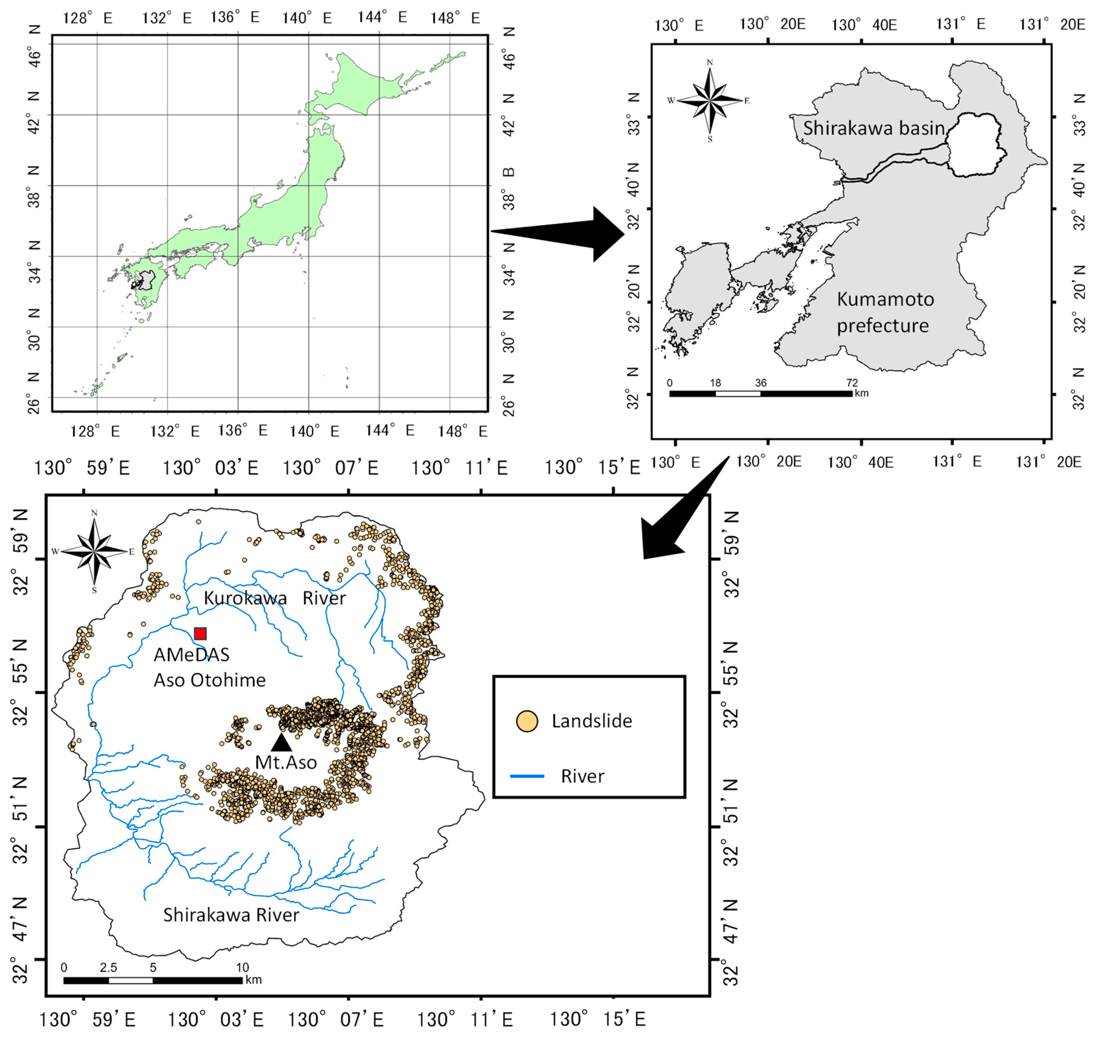
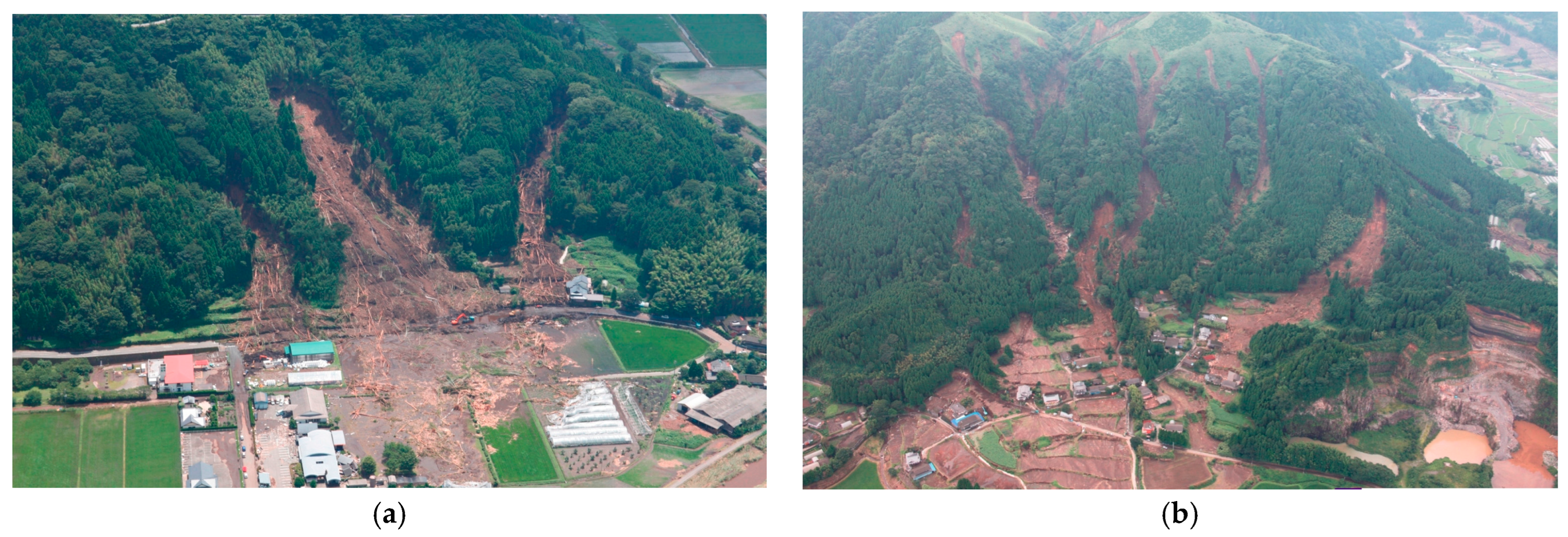
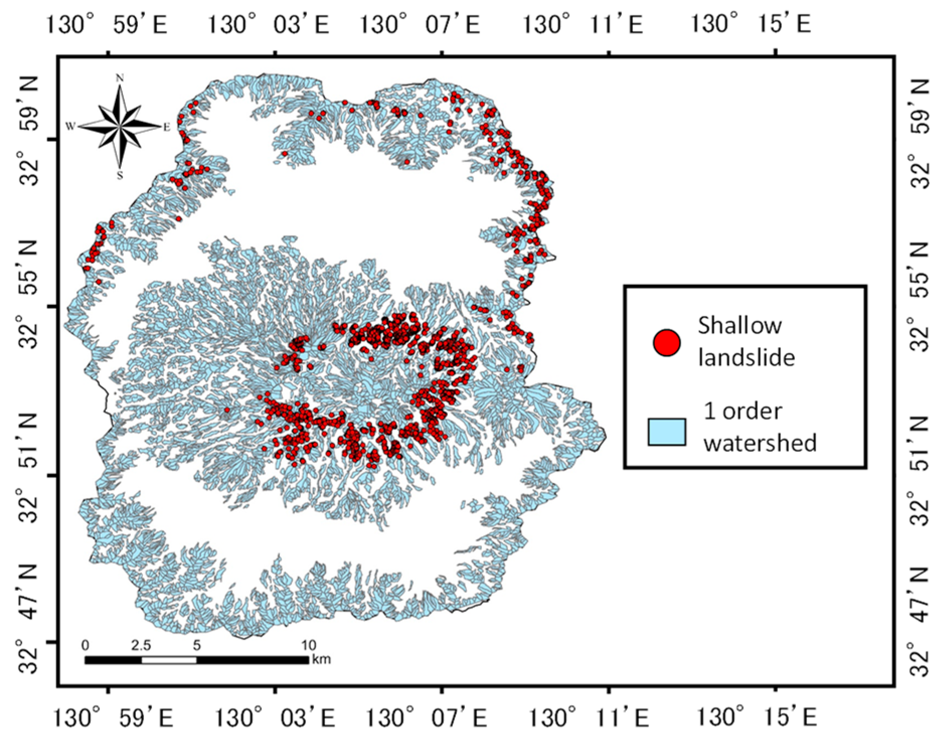
2. Study Area
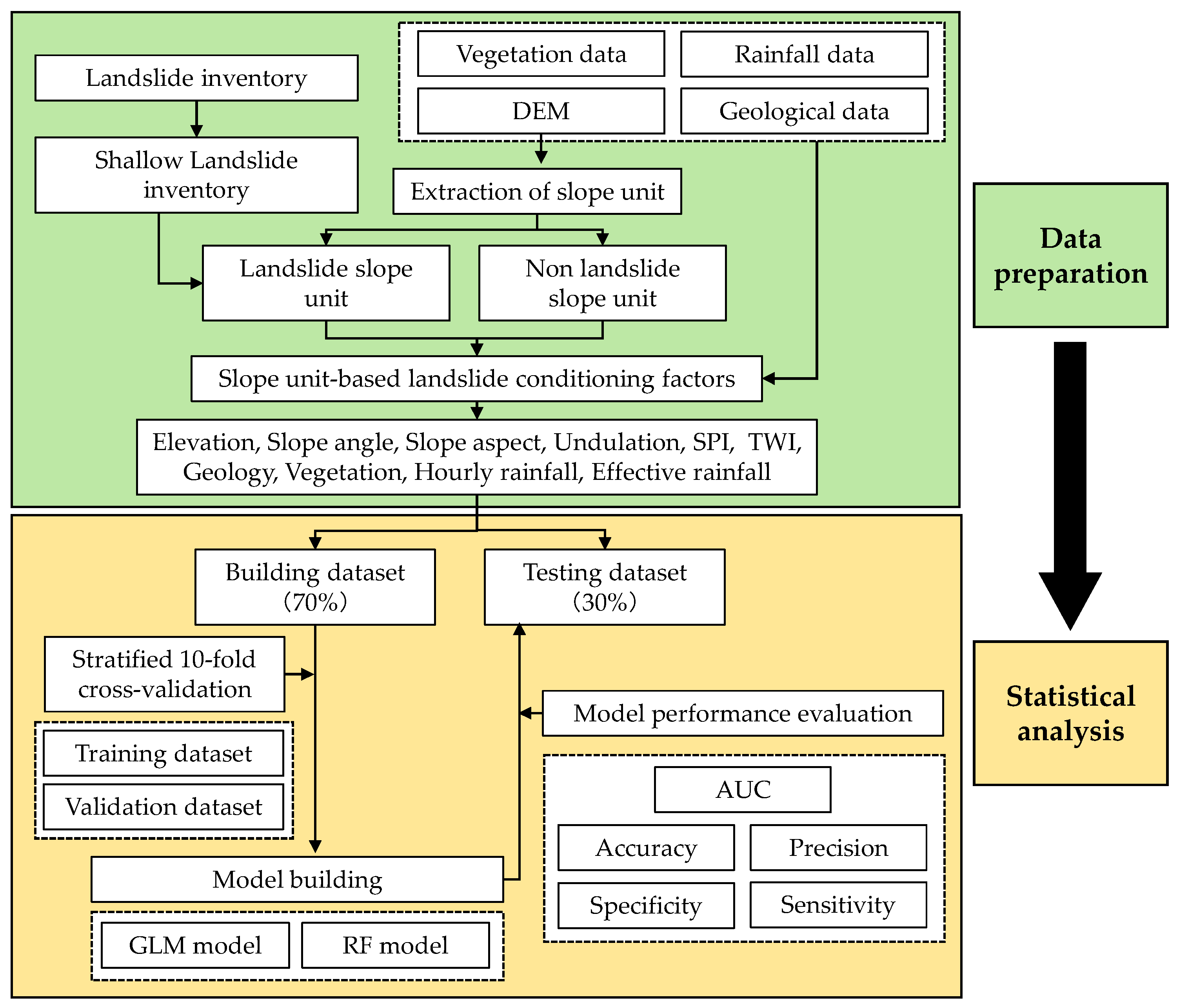
3. Materials and Methods
3.1. Extraction of Shallow Landslides Data and Creation of Slope Units
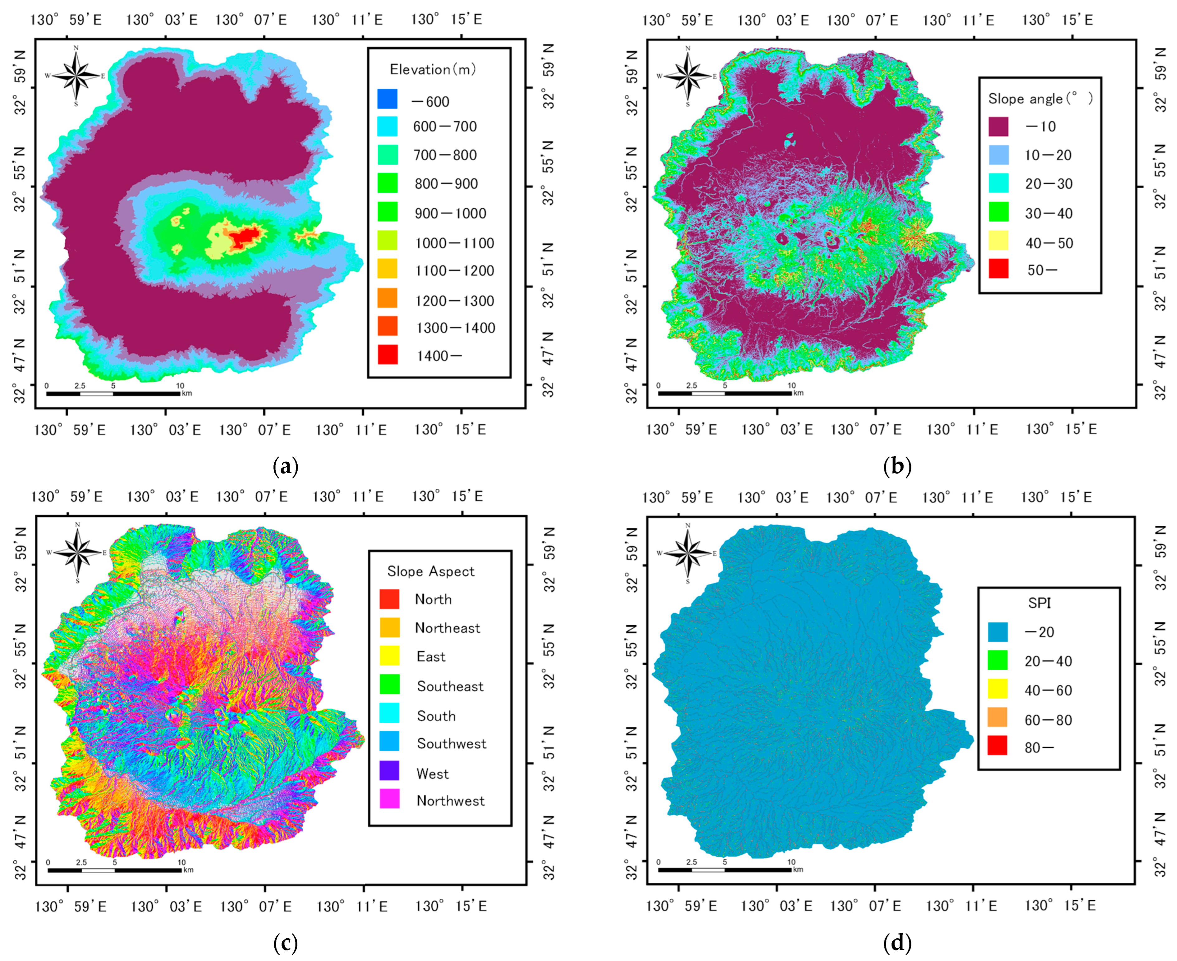
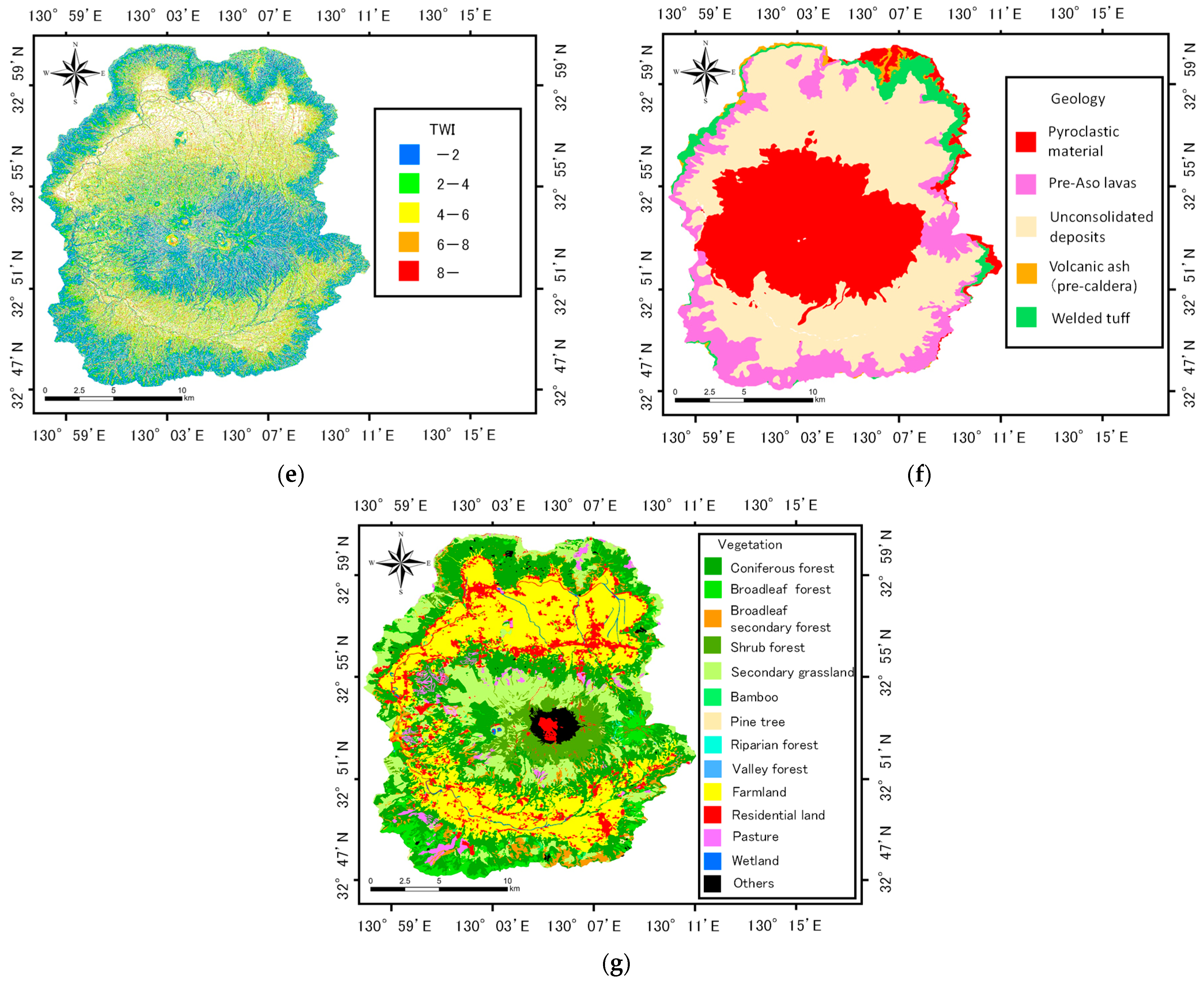
3.2. Creating Data on Primary Factors for Shallow Landslides
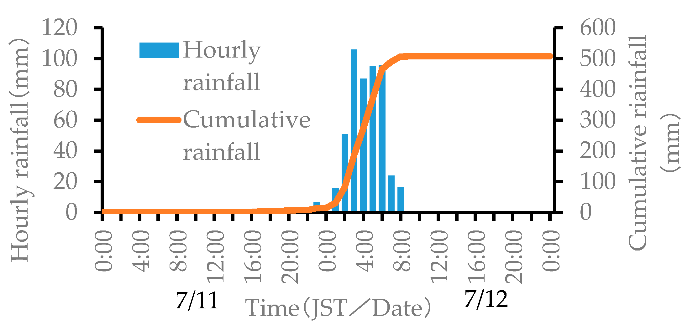
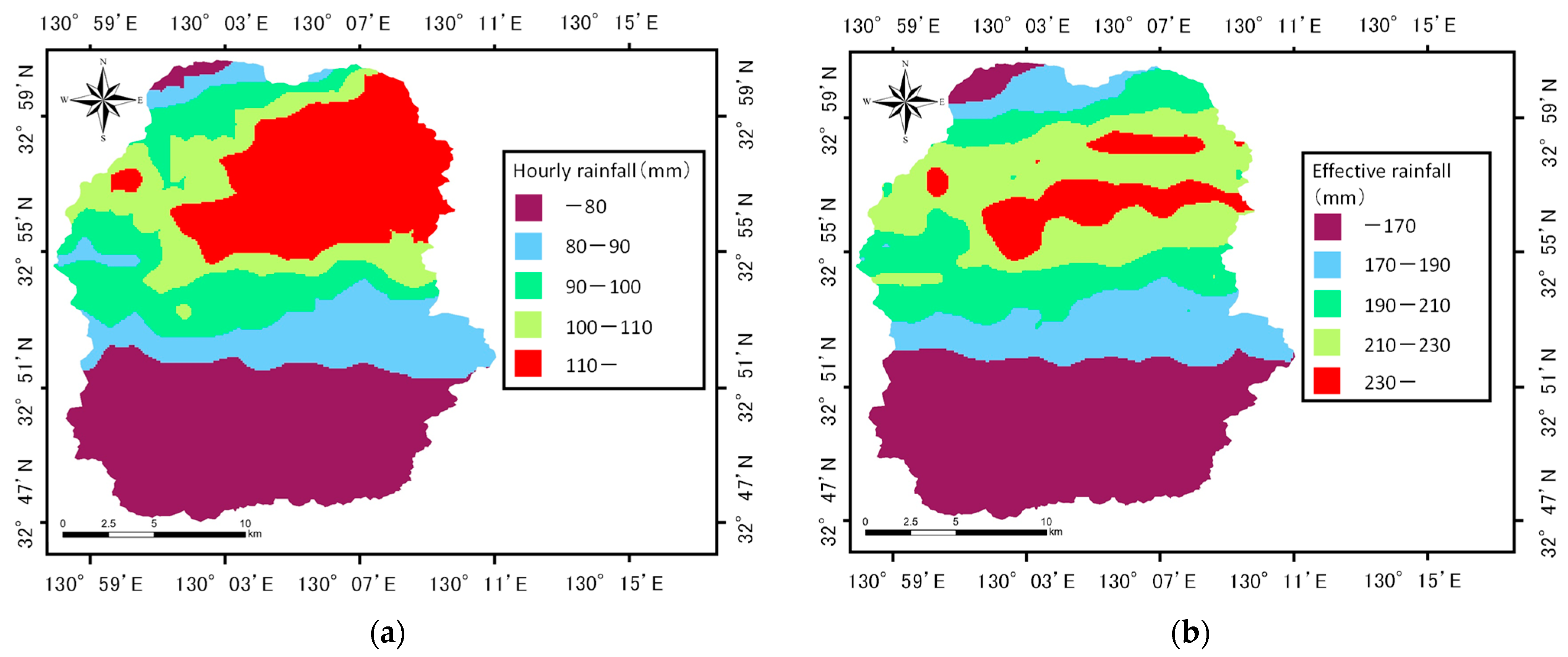
3.3. Creating Data on Triggering Factors for Shallow Landslides
3.4. Statistical Analysis
3.4.1. Preparation of Model Building Dataset and Testing Dataset
3.4.2. Multicollinearity
3.4.3. Generalized Linear Model
3.4.4. Random Forest
3.4.5. Model Performance Evaluation
4. Results
4.1. Correlation Analysis
4.2. Generalized Linear Model
4.3. Random Forest
5. Discussion
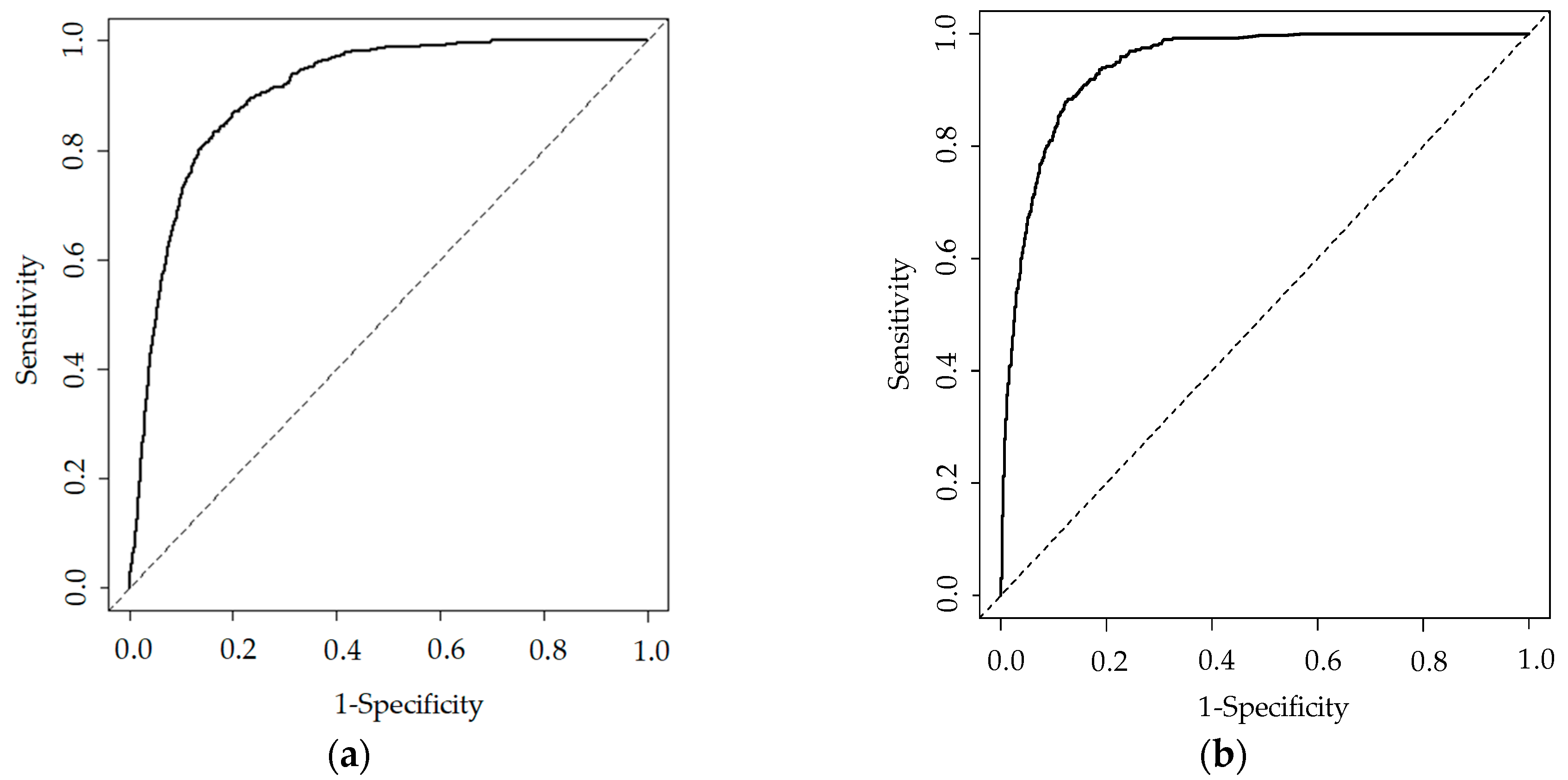
5.1. Model Performance Evaluation
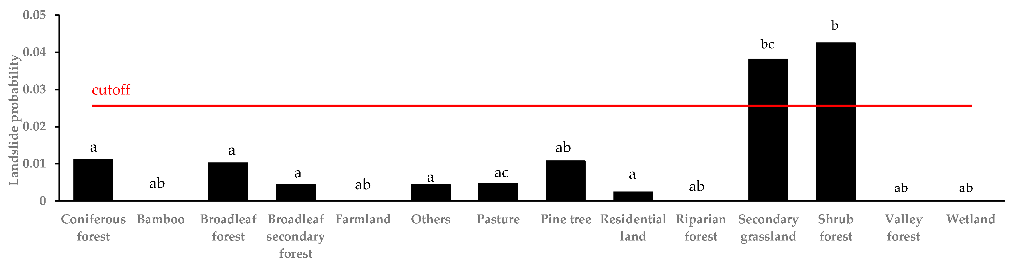
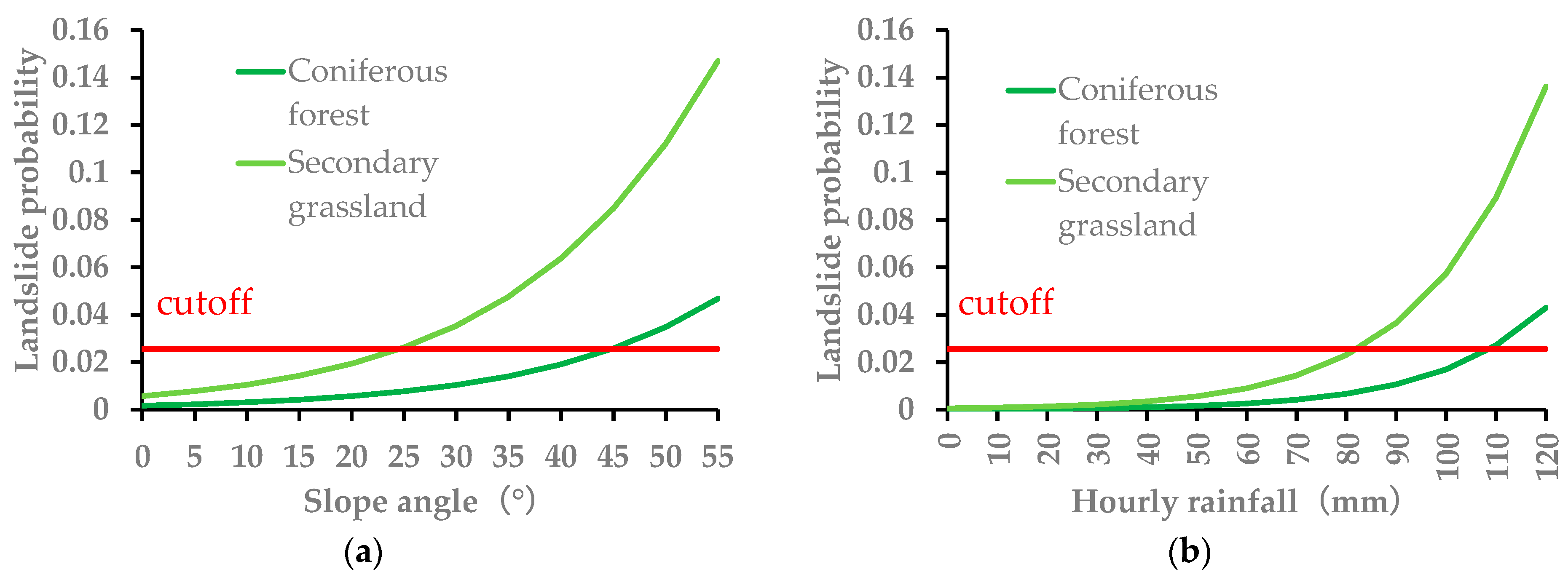
5.2. Impact of Vegetation on Shallow Landslides
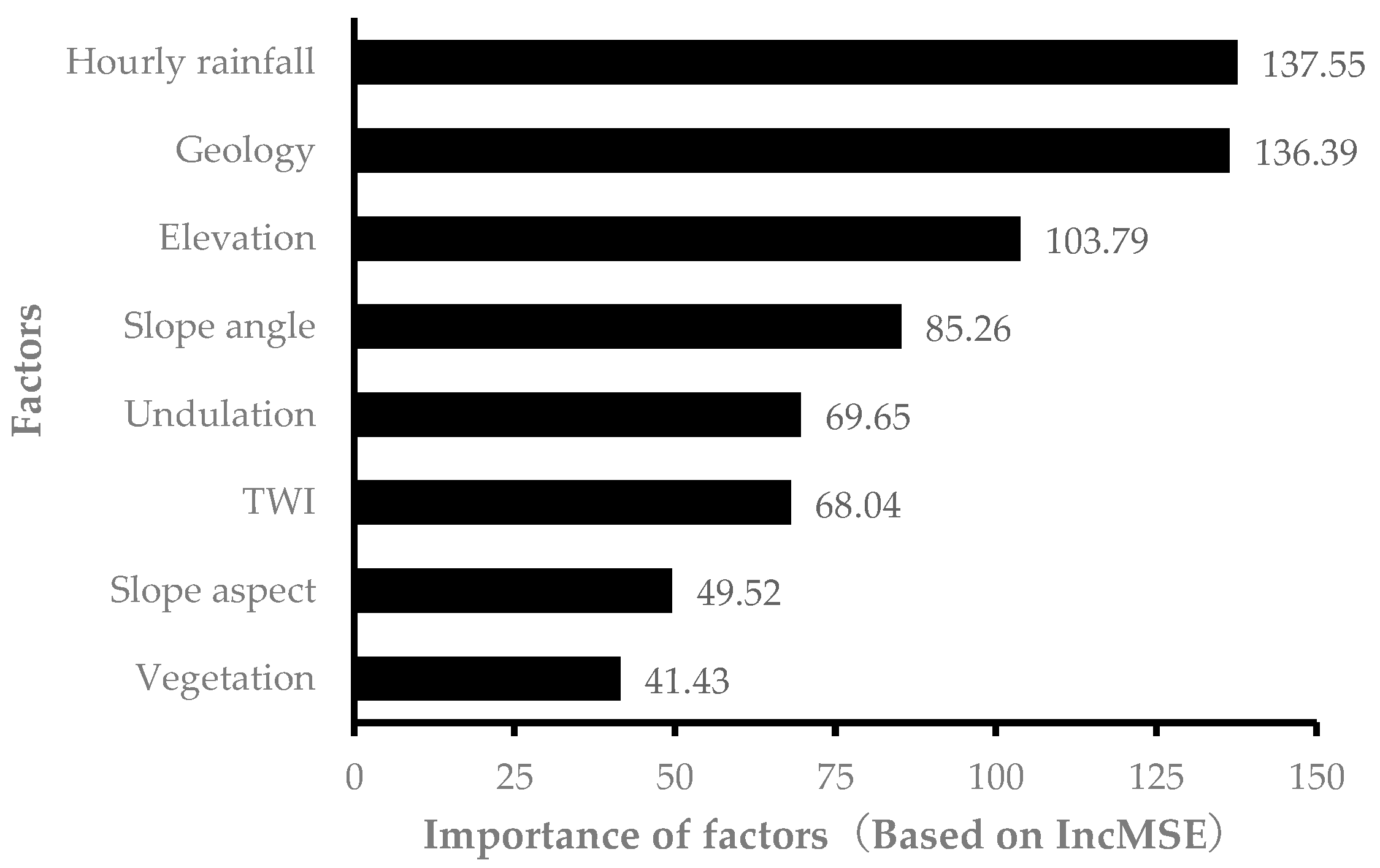
5.3. Importance of Contributing Factors
6. Conclusions
Author Contributions
Funding
Data Availability Statement
Acknowledgments
Conflicts of Interest
Appendix A

| Factors | Coniferous Forest | Bamboo | Broadleaf Forest | Broadleaf Secondary Forest | Farmland | Others | Pasture |
|---|---|---|---|---|---|---|---|
| Coniferous forest | - | −13.08 | −0.09 | 0.94 | −12.47 | −0.95 | −0.87 |
| Bamboo | 671.3 | - | 12.99 | 12.14 | 0.60 | 12.13 | 12.21 |
| Broadleaf forest | 0.26 | 671.3 | - | −0.85 | 141 | −0.86 | −0.78 |
| Broadleaf secondary forest | 0.35 | 671.3 | 0.42 | - | 141 | −0.01 | 0.07 |
| Farmland | 141 | 686 | 12.38 | 11.53 | - | 11.53 | 11.61 |
| Others | 0.37 | 671.3 | 0.43 | 0.49 | 141 | - | 0.08 |
| Pasture | 0.72 | 671.3 | 0.76 | 0.79 | 141 | 0.79 | - |
| Pine tree | 1.02 | 671.3 | 1.04 | 1.07 | 141 | 1.07 | 1.24 |
| Residential land | 0.59 | 671.3 | 0.63 | 0.68 | 141 | 0.67 | 0.92 |
| Riparian forest | 1258 | 1426 | 1258.00 | 1258.00 | 1266 | 1258.00 | 1258.00 |
| Secondary grassland | 0.11 | 671.3 | 0.25 | 0.35 | 141 | 0.35 | 0.71 |
| Shrub forest | 0.13 | 671.3 | 0.26 | 0.35 | 141 | 0.34 | 0.72 |
| Valley forest | 1829 | 1948 | 1829 | 1829 | 1834 | 1829 | 1829 |
| Wetland | 2229 | 2328 | 2229 | 2229 | 2233 | 2229 | 2229 |
| Factors | Pine Tree | Residential Land | Riparian Forest | Secondary Grassland | Shrub Forest | Valley Forest | Wetland |
|---|---|---|---|---|---|---|---|
| Coniferous forest | −0.04 | −1.54 | −13.28 | 1.26 | 1.37 | −14.34 | −12.36 |
| Bamboo | 13.04 | 11.54 | −0.20 | 14.33 | 14.45 | −1.27 | 0.72 |
| Broadleaf forest | 0.05 | −1.45 | −13.19 | 1.34 | 1.46 | −14.25 | −12.27 |
| Broadleaf secondary forest | 0.90 | −0.60 | −12.34 | 2.20 | 2.31 | −13.4 | −11.42 |
| Farmland | 12.44 | 10.93 | −0.80 | 13.73 | 13.84 | −1.87 | 0.11 |
| Others | 0.91 | −0.59 | −12.33 | 2.20 | 2.32 | −13.4 | −11.41 |
| Pasture | 0.83 | −0.67 | −12.41 | 2.12 | 2.24 | −13.48 | −11.49 |
| Pine tree | - | −1.50 | −13.24 | 1.29 | 1.41 | −14.31 | −12.32 |
| Residential land | 1.17 | - | −11.74 | 2.80 | 2.91 | −12.80 | −10.82 |
| Riparian forest | 1258.00 | 1258.00 | - | 14.53 | 14.65 | −1.07 | 0.92 |
| Secondary grassland | 1.01 | 0.58 | 1258 | - | 0.11 | −15.6 | −13.61 |
| Shrub forest | 1.02 | 0.58 | 1258 | 0.09 | - | −15.71 | −13.73 |
| Valley forest | 1829 | 1829 | 2220 | 1829 | 1829 | - | 1.98 |
| Wetland | 2229 | 2229 | 2559 | 2229 | 2229 | 2883 | - |
References
- Murgia, I.; Giadrossich, F.; Mao, Z.; Cohen, D.; Capra, G.F.; Schwarz, M. Modeling shallow landslides and root reinforcement: A review. Ecol. Eng. 2022, 181, 106671. [Google Scholar] [CrossRef]
- Ran, Q.; Hong, Y.; Li, W.; Gao, J. A modelling study of rainfall-induced shallow landslide mechanisms under different rainfall characteristics. J. Hydrol. 2018, 563, 790–801. [Google Scholar] [CrossRef]
- Persichillo, M.G.; Bordoni, M.; Meisina, C. The role of land use changes in the distribution of shallow landslides. Sci. Total Environ. 2017, 574, 924–937. [Google Scholar] [CrossRef] [PubMed]
- Cohen, D.; Schwarz, M. Tree-root control of shallow landslides. Earth Surf. Dyn. 2017, 5, 451–477. [Google Scholar] [CrossRef]
- Schwarz, M.; Cohen, D.; Or, D. Pullout tests of root analogs and natural root bundles in soil: Experiments and modeling. J. Geophys. Res. Atmos. 2011, 116, F02007. [Google Scholar] [CrossRef]
- Liu, C.; Bi, H.; Wang, D.; Li, X. Stability Reinforcement of Slopes Using Vegetation Considering the Existence of Soft Rock. Appl. Sci. 2021, 11, 9228. [Google Scholar] [CrossRef]
- Getzner, M.; Gutheil-Knopp-Kirchwald, G.; Kreimer, E.; Kirchmeir, H.; Huber, M. Gravitational natural hazards: Valuing the protective function of Alpine forests. For. Policy Econ. 2017, 80, 150–159. [Google Scholar] [CrossRef]
- Montgomery, D.R.; Dietrich, W.E. A physically based model for the topographic control on shallow landsliding. Water Resour. Res. 1994, 30, 1153–1171. [Google Scholar] [CrossRef]
- Wu, W.; Sidle, R.C. A distributed slope stability model for steep forested basins. Water Resour. Res. 1995, 31, 2097–2110. [Google Scholar] [CrossRef]
- Schwarz, M.; Cohen, D.; Or, D. Spatial characterization of root reinforcement at stand scale: Theory and case study. Geomorphology 2012, 171–172, 190–200. [Google Scholar] [CrossRef]
- Mao, Z.; Jourdan, C.; Bonis, M.-L.; Pailler, F.; Rey, H.; Saint-André, L.; Stokes, A. Modelling root demography in heterogeneous mountain forests and applications for slope stability analysis. Plant Soil 2012, 363, 357–382. [Google Scholar] [CrossRef]
- Schwarz, M.; Lehmann, P.; Or, D. Quantifying lateral root reinforcement in steep slopes—From a bundle of roots to tree stands. Earth Surf. Process. Landf. 2010, 35, 354–367. [Google Scholar] [CrossRef]
- Giadrossich, F.; Schwarz, M.; Marden, M.; Marrosu, R.; Phillips, C. Minimum representative root distribution sampling for calculating slope stability in Pinus radiata D.Don plantations in New Zealand. N. Z. J. For. Sci. 2020, 50, 5. [Google Scholar] [CrossRef]
- Schwarz, M.; Cohen, D.; Or, D. Root-soil mechanical interactions during pullout and failure of root bundles. J. Geophys. Res. Atmos. 2010, 115, F04035. [Google Scholar] [CrossRef]
- Gehring, E.; Conedera, M.; Maringer, J.; Giadrossich, F.; Guastini, E.; Schwarz, M. Shallow landslide disposition in burnt European beech (Fagus sylvatica L.) forests. Sci. Rep. 2019, 9, 8638. [Google Scholar] [CrossRef] [PubMed]
- Vergani, C.; Schwarz, M.; Soldati, M.; Corda, A.; Giadrossich, F.; Chiaradia, E.A.; Morando, P.; Bassanelli, C. Root reinforcement dynamics in subalpine spruce forests following timber harvest: A case study in Canton Schwyz, Switzerland. CATENA 2016, 143, 275–288. [Google Scholar] [CrossRef]
- Giadrossich, F.; Cohen, D.; Schwarz, M.; Seddaiu, G.; Contran, N.; Lubino, M.; Valdés-Rodríguez, O.A.; Niedda, M. Modeling bio-engineering traits of Jatropha curcas L. Ecol. Eng. 2016, 89, 40–48. [Google Scholar] [CrossRef]
- Merghadi, A.; Yunus, A.P.; Dou, J.; Whiteley, J.; ThaiPham, B.; Bui, D.T.; Avtar, R.; Abderrahmane, B. Machine learning methods for landslide susceptibility studies: A comparative overview of algorithm performance. Earth Sci. Rev. 2020, 207, 103225. [Google Scholar] [CrossRef]
- Guzzetti, F.; Reichenbach, P.; Ardizzone, F.; Cardinali, M.; Galli, M. Estimating the quality of landslide susceptibility models. Geomorphology 2006, 81, 166–184. [Google Scholar] [CrossRef]
- Abeysiriwardana, H.D.; Gomes, P.I.A. Integrating vegetation indices and geo-environmental factors in GIS-based landslide-susceptibility mapping: Using logistic regression. J. Mt. Sci. 2022, 19, 477–492. [Google Scholar] [CrossRef]
- Sun, X.; Chen, J.; Han, X.; Bao, Y.; Zhan, J.; Peng, W. Application of a GIS-based slope unit method for landslide susceptibility mapping along the rapidly uplifting section of the upper Jinsha River, South-Western China. Bull. Eng. Geol. Environ. 2019, 79, 533–549. [Google Scholar] [CrossRef]
- Zhao, P.; Masoumi, Z.; Kalantari, M.; Aflaki, M.; Mansourian, A. A GIS-Based Landslide Susceptibility Mapping and Variable Importance Analysis Using Artificial Intelligent Training-Based Methods. Remote Sens. 2022, 14, 211. [Google Scholar] [CrossRef]
- Zhao, Z.; Liu, Z.Y.; Xu, C. Slope Unit-Based Landslide Susceptibility Mapping Using Certainty Factor, Support Vector Machine, Random Forest, CF-SVM and CF-RF Models. Front. Earth Sci. 2021, 9, 589630. [Google Scholar] [CrossRef]
- Nandi, A.; Shakoor, A. A GIS-based landslide susceptibility evaluation using bivariate and multivariate statistical analyses. Eng. Geol. 2010, 110, 11–20. [Google Scholar] [CrossRef]
- Neuhäuser, B.; Damm, B.; Terhorst, B. GIS-based assessment of landslide susceptibility on the base of the Weights-of-Evidence model. Landslides 2011, 9, 511–528. [Google Scholar] [CrossRef]
- Moos, C.; Bebi, P.; Graf, F.; Mattli, J.; Rickli, C.; Schwarz, M. How does forest structure affect root reinforcement and susceptibility to shallow landslides? Earth Surf. Process. Landf. 2015, 41, 951–960. [Google Scholar] [CrossRef]
- Zhang, Y.; Shen, C.; Zhou, S.; Luo, X. Analysis of the Influence of Forests on Landslides in the Bijie Area of Guizhou. Forests 2022, 13, 1136. [Google Scholar] [CrossRef]
- Teerawattanasuk, C.; Maneecharoen, J.; Bergado, D.T.; Voottipruex, P.; Le, G.L. Root strength measurements of Vetiver and Ruzi grasses. Lowl. Technol. Int. 2014, 16, 71–80. [Google Scholar] [CrossRef] [PubMed]
- Hao, G.; Liu, X.; Zhang, Q.; Xiang, L.; Yu, B. Optimum Selection of Soil-Reinforced Herbaceous Plants Considering Plant Growth and Distribution Characteristics. J. Soil Sci. Plant Nutr. 2022, 22, 1743–1757. [Google Scholar] [CrossRef]
- Miyabuchi, Y.; Sugiyama, S. 90,000-year phytolith record from tephra section at the northeastern rim of Aso caldera, Japan. Quat. Int. 2011, 246, 239–246. [Google Scholar] [CrossRef]
- Miyabuchi, Y.; Sugiyama, S.; Nagaoka, Y. Vegetation and fire history during the last 30,000 years based on phytolith and macroscopic charcoal records in the eastern and western areas of Aso Volcano, Japan. Quat. Int. 2010, 254, 28–35. [Google Scholar] [CrossRef]
- Koyama, A.; Koyanagi, T.F.; Akasaka, M.; Takada, M.; Okabe, K. Combined burning and mowing for restoration of abandoned semi-natural grasslands. Appl. Veg. Sci. 2016, 20, 40–49. [Google Scholar] [CrossRef]
- Liu, J.; Wu, Z.; Zhang, H. Analysis of Changes in Landslide Susceptibility according to Land Use over 38 Years in Lixian County, China. Sustainability 2021, 13, 10858. [Google Scholar] [CrossRef]
- Kokutse, N.K.; Temgoua, A.G.T.; Kavazović, Z. Slope stability and vegetation: Conceptual and numerical investigation of mechanical effects. Ecol. Eng. 2016, 86, 146–153. [Google Scholar] [CrossRef]
- Koyanagi, K.; Gomi, T.; Sidle, R.C. Characteristics of landslides in forests and grasslands triggered by the 2016 Kumamoto earthquake. Earth Surf. Process. Landforms 2019, 45, 893–904. [Google Scholar] [CrossRef]
- Kamp, U.; Growley, B.J.; Khattak, G.A.; Owen, L.A. GIS-based landslide susceptibility mapping for the 2005 Kashmir earthquake region. Geomorphology 2008, 101, 631–642. [Google Scholar] [CrossRef]
- Miyabuchi, Y. Landslides Triggered by the July 2012 Torrential Rain in Aso Caldera, Southwestern Japan. J. Geogr. (Chigaku Zasshi) 2012, 121, 1073–1080. [Google Scholar] [CrossRef]
- National Research Institute for Earth Science and Disaster Resilience. Sediment Movement Distribution Map due to the Ku-mamoto Earthquake. Available online: http://www.bosai.go.jp/mizu/dosha.html (accessed on 24 May 2023).
- Asada, H.; Minagawa, T.; Koyama, A.; Ichiyanagi, H. Factor analysis of surface collapse on slopes caused by the July 2017 Northern Kyushu Heavy Rain. Ecol. Civ. Eng. 2020, 23, 185–196. [Google Scholar] [CrossRef]
- Chen, W.; Sun, Z.; Han, J. Landslide Susceptibility Modeling Using Integrated Ensemble Weights of Evidence with Logistic Regression and Random Forest Models. Appl. Sci. 2019, 9, 171. [Google Scholar] [CrossRef]
- Lee, S.; Min, K. Statistical analysis of landslide susceptibility at Yongin, Korea. Environ. Geol. 2001, 40, 1095–1113. [Google Scholar] [CrossRef]
- Capitani, M.; Ribolini, A.; Bini, M. The slope aspect: A predisposing factor for landsliding? C. R. Geosci. 2013, 345, 427–438. [Google Scholar] [CrossRef]
- Takezawa, N.; Uchida, T.; Ishizuka, T.; Honma, S.; Kobayashi, Y.; Miyajima, M. Assessing of scale and susceptibility of landslides to earthquake focused on slope relief. J. Jpn. Soc. Eros. Control Eng. 2013, 65, 22–29. [Google Scholar]
- Pourghasemi, H.R.; Mohammady, M.; Pradhan, B. Landslide susceptibility mapping using index of entropy and conditional probability models in GIS: Safarood Basin, Iran. CATENA 2012, 97, 71–84. [Google Scholar] [CrossRef]
- Jaafari, A. LiDAR-supported prediction of slope failures using an integrated ensemble weights-of-evidence and analytical hierarchy process. Environ. Earth Sci. 2018, 77, 42. [Google Scholar] [CrossRef]
- Ohlmacher, G.C. Plan curvature and landslide probability in regions dominated by earth flows and earth slides. Eng. Geol. 2007, 91, 117–134. [Google Scholar] [CrossRef]
- Uchida, T.; Mori, N.; Tamura, K.; Terada, H.; Takiguchi, S.; Kamee, K. The role of data preparation on shallow landslide pre-diction. Jpn. Soc. Eros. Control Eng. 2009, 62, 23–31. [Google Scholar] [CrossRef]
- Safaei, M.; Omar, H.; Huat, B.K.; Yousof, Z.B.M. Relationship between Lithology Factor and landslide occurrence based on Information Value (IV) and Frequency Ratio (FR) approaches—Case study in North of Iran. Electron. J. Geotech. Eng. 2012, 17, 79–90. [Google Scholar]
- Oka, N.; Kazama, H.; Akutagawa, S.; Oda, M. Site characteristics of slope failures caused by rainfall. Doboku Gakkai Ronbunshu 1993, 1993, 11–20. [Google Scholar] [CrossRef]
- Seyed, A.H.; Reza, L.; Majid, L.; Ataollah, K.; Aidin, P. The effect of terrain factors on landslide features along forest road. Afr. J. Biotechnol. 2011, 10, 14108–14115. [Google Scholar] [CrossRef]
- Moore, I.D.; Grayson, R.B.; Ladson, A.R. Digital terrain modelling: A review of hydrological, geomorphological, and biological applications. Hydrol. Processes 1991, 5, 3–30. [Google Scholar] [CrossRef]
- National Institute of Advanced Industrial Science and Technology. Geological Map of Aso Volcano. Available online: https://www.gsj.jp/Map/JP/volcano.html (accessed on 24 May 2023).
- Furukawa, K.; Miyoshi, M.; Shinmura, T.; Shibata, T.; Arakawa, Y. Geology and petrology of the pre-Aso volcanic rocks distributed in the NW wall of Aso Caldera: Eruption style and magma plumbing system of the pre-caldera volcanism. J. Geol. Soc. Jpn. 2009, 115, 658–671. [Google Scholar] [CrossRef]
- Ono, K. Geology of the Eastern Part of Aso Caldera, Central Kyushu, Southwest Japan. J. Geol. Soc. Jpn. 1965, 71, 541–553. [Google Scholar] [CrossRef]
- Ono, K.; Watanabe, K. Geological Map of Aso Volcano (1:50,000); Geological Map of Volcanoes 4; Geological Survey of Japan: Tsukuba, Japan, 1985.
- Miyabuchi, Y. Post-caldera explosive activity inferred from improved 67–30ka tephrostratigraphy at Aso Volcano, Japan. J. Volcanol. Geotherm. Res. 2011, 205, 94–113. [Google Scholar] [CrossRef]
- Ministry of Environment. Natural Environment Survey Web-GIS. Available online: http://gis.biodic.go.jp/webgis/index.html (accessed on 24 May 2023).
- Dai, F.; Lee, C. Frequency–volume relation and prediction of rainfall-induced landslides. Eng. Geol. 2001, 59, 253–266. [Google Scholar] [CrossRef]
- Hong, Y.; Hiura, H.; Shino, K.; Sassa, K.; Suemine, A.; Fukuoka, H.; Wang, G. The influence of intense rainfall on the activity of large-scale crystalline schist landslides in Shikoku Island, Japan. Landslides 2005, 2, 97–105. [Google Scholar] [CrossRef]
- Yano, K. Study of the Method for Setting Standard Rainfall of Debris Flow by the Reform of Antecedent Rain. Jpn. Soc. Eros. Control Eng. 1990, 43, 3–13. [Google Scholar] [CrossRef]
- Terada, H.; Nakaya, H. Operating Methods of Critical Rainfall for Warning and Evacuation from Sediment-Related Disasters. Technical Note of National Institute for Land and Infrastructure Management; Ministry of Land, Infrastructure, Transport and Tourism: Tokyo, Japan, 2001; Volume 5, pp. 1–58.
- Brand, E.W.; Premchitt, J.; Phillipson, H.B. Relationship between rainfall and landslides in Hong Kong. In Proceedings of the Fourth International Symposium on Landslides, Toronto, ON, Canada, 16–21 September 1984; Volume 1, pp. 377–384. [Google Scholar]
- Japan Meteorological Agency: Japan Meteorological Business Support Center. Available online: http://www.jma.go.jp/jma/index.html (accessed on 24 May 2023).
- Dutton, A.L.; Loague, K.; Wemple, B.C. Simulated effect of a forest road on near-surface hydrologic response and slope stability. Earth Surf. Process. Landf. 2005, 30, 325–338. [Google Scholar] [CrossRef]
- Dou, J.; Bui, D.T.; Yunus, A.P.; Jia, K.; Song, X.; Revhaug, I.; Xia, H.; Zhu, Z. Optimization of Causative Factors for Landslide Susceptibility Evaluation Using Remote Sensing and GIS Data in Parts of Niigata, Japan. PLoS ONE 2015, 10, e0133262. [Google Scholar] [CrossRef]
- Wang, Y.; Sun, D.; Wen, H.; Zhang, H.; Zhang, F. Comparison of Random Forest Model and Frequency Ratio Model for Landslide Susceptibility Mapping (LSM) in Yunyang County (Chongqing, China). Int. J. Environ. Res. Public Health 2020, 17, 4206. [Google Scholar] [CrossRef]
- Liu, R.; Yang, X.; Xu, C.; Wei, L.; Zeng, X. Comparative Study of Convolutional Neural Network and Conventional Machine Learning Methods for Landslide Susceptibility Mapping. Remote Sens. 2022, 14, 321. [Google Scholar] [CrossRef]
- Park, S.; Hamm, S.-Y.; Kim, J. Performance Evaluation of the GIS-Based Data-Mining Techniques Decision Tree, Random Forest, and Rotation Forest for Landslide Susceptibility Modeling. Sustainability 2019, 11, 5659. [Google Scholar] [CrossRef]
- Kalantar, B.; Ueda, N.; Saeidi, V.; Ahmadi, K.; Halin, A.A.; Shabani, F. Landslide Susceptibility Mapping: Machine and Ensemble Learning Based on Remote Sensing Big Data. Remote Sens. 2020, 12, 1737. [Google Scholar] [CrossRef]
- Li, X.; Wang, Y. Applying various algorithms for species distribution modelling. Integr. Zool. 2013, 8, 124–135. [Google Scholar] [CrossRef] [PubMed]
- Breiman, L. Random forests. Mach. Learn. 2001, 45, 5–32. [Google Scholar] [CrossRef]
- Efron, B. Bootstrap Methods: Another Look at the Jackknife. Ann. Stat. 1979, 7, 1–26. [Google Scholar] [CrossRef]
- Trigila, A.; Iadanza, C.; Esposito, C.; Scarascia-Mugnozza, G. Comparison of Logistic Regression and Random Forests techniques for shallow landslide susceptibility assessment in Giampilieri (NE Sicily, Italy). Geomorphology 2015, 249, 119–136. [Google Scholar] [CrossRef]
- Breiman, L. Statistical Modeling: The Two Cultures (with comments and a rejoinder by the author). Stat. Sci. 2001, 16, 199–231. [Google Scholar] [CrossRef]
- Chen, W.; Zhang, S.; Li, R.; Shahabi, H. Performance evaluation of the GIS-based data mining techniques of best-first decision tree, random forest, and naïve Bayes tree for landslide susceptibility modeling. Sci. Total Environ. 2018, 644, 1006–1018. [Google Scholar] [CrossRef]
- Pearce, J.; Ferrier, S. Evaluating the predictive performance of habitat models developed using logistic regression. Ecol. Model. 2000, 133, 225–245. [Google Scholar] [CrossRef]
- Sun, D.; Xu, J.; Wen, H.; Wang, D. Assessment of landslide susceptibility mapping based on Bayesian hyperparameter op-timization: A comparison between logistic regression and random forest. Eng. Geol. 2021, 281, 105972. [Google Scholar] [CrossRef]
- Chawla, N.V.; Bowyer, K.W.; Hall, L.O.; Kegelmeyer, W.P. SMOTE: Synthetic Minority Over-sampling Technique. J. Artif. Intell. Res. 2002, 16, 321–357. [Google Scholar] [CrossRef]
- Keim, R.F.; Skaugset, A.E. Modelling effects of forest canopies on slope stability. Hydrol. Process. 2003, 17, 1457–1467. [Google Scholar] [CrossRef]
- Dhakal, A.S.; Sidle, R.C. Pore water pressure assessment in a forest watershed: Simulations and distributed field measurements related to forest practices. Water Resour. Res. 2004, 40, W02405. [Google Scholar] [CrossRef]
- Ji, J.; Kokutse, N.; Genet, M.; Fourcaud, T.; Zhang, Z. Effect of spatial variation of tree root characteristics on slope stability. A case study on Black Locust (Robinia pseudoacacia) and Arborvitae (Platycladus orientalis) stands on the Loess Plateau, China. Catena 2012, 92, 139–154. [Google Scholar] [CrossRef]
- Löbmann, M.T.; Geitner, C.; Wellstein, C.; Zerbe, S. The influence of herbaceous vegetation on slope stability—A review. Earth-Sci. Rev. 2020, 209, 103328. [Google Scholar] [CrossRef]
- Gomi, T.; Sidle, R.C.; Noguchi, S.; Negishi, J.N.; Nik, A.R.; Sasaki, S. Sediment and wood accumulations in humid tropical headwater streams: Effects of logging and riparian buffers. For. Ecol. Manag. 2006, 224, 166–175. [Google Scholar] [CrossRef]
- De Vita, P.; Napolitano, E.; Godt, J.W.; Baum, R.L. Deterministic estimation of hydrological thresholds for shallow landslide initiation and slope stability models: Case study from the Somma-Vesuvius area of southern Italy. Landslides 2012, 10, 713–728. [Google Scholar] [CrossRef]
- Feizizadeh, B.; Blaschke, T.; Nazmfar, H.; Moghaddam, M.R. Landslide Susceptibility Mapping for the Urmia Lake basin, Iran: A multi-Criteria Evaluation Approach using GIS. Int. J. Environ. Res. 2013, 7, 319–336. [Google Scholar] [CrossRef]


| Factors | Data Source | Data Type | Value Range |
|---|---|---|---|
| Elevation | DEM | Continuous | 246.51–1587.16 |
| Slope angle | DEM | Continuous | 0.01–67.57 |
| Slope aspect | DEM | Categorical | n/a |
| Undulation | DEM | Continuous | 0.00–342.00 |
| SPI | DEM | Continuous | 0.00–106,087.27 |
| TWI | DEM | Continuous | −0.88–11.88 |
| Geology | [53] | Categorical | n/a |
| Vegetation | [64] | Categorical | n/a |
| Hourly rainfall | [65] | Continuous | 53.4–124.46 |
| Effective rainfall | [65] | Continuous | 57.96–249.86 |
| True Condition | |||
|---|---|---|---|
| Landslide | Non-Landslide | ||
| Prediction Condition | Landslide | TP | FP |
| Non-landslide | FN | TN | |
| Factors | Variance Inflation Factors (VIF) | |
|---|---|---|
| Elevation | 2.03 | 2.01 |
| Slope angle | 3.32 | 3.37 |
| Slope aspect | 1.12 | 1.13 |
| Undulation | 1.83 | 1.83 |
| SPI | 1.00 | 1.00 |
| TWI | 1.69 | 1.73 |
| Geology | 1.85 | 1.83 |
| Vegetation | 2.33 | 2.24 |
| Hourly rainfall | 1.61 | n/a |
| Effective rainfall | n/a | 1.49 |
| Factor | Estimate | Std. Error | z Value | p-Value | |
|---|---|---|---|---|---|
| (Intercept) | −9.87 | 0.62 | −15.96 | <0.05 | |
| Elevation | 0.00 | 0.00 | −3.52 | <0.05 | |
| Slope angle | 0.06 | 0.01 | 11.78 | <0.05 | |
| Slope aspect | east | 1.09 | 0.43 | 2.54 | <0.05 |
| northeast | 0.36 | 0.44 | 0.83 | 0.41 | |
| northwest | 0.82 | 0.43 | 1.91 | 0.06 | |
| south | 0.87 | 0.43 | 2.03 | <0.05 | |
| southeast | 0.84 | 0.43 | 1.95 | 0.05 | |
| southwest | 0.83 | 0.43 | 1.92 | 0.06 | |
| west | 0.80 | 0.43 | 1.86 | 0.06 | |
| Undulation | 0.01 | 0.00 | 9.75 | <0.05 | |
| TWI | −0.40 | 0.05 | −8.63 | <0.05 | |
| Geology | Pre-Aso lavas | −2.56 | 0.15 | −17.10 | <0.05 |
| Unconsolidated deposits | −2.42 | 0.34 | −7.07 | <0.05 | |
| Welded tuff | −1.17 | 0.32 | −3.62 | <0.05 | |
| Volcanic ash (pre-caldera) | −1.37 | 0.12 | −11.07 | <0.05 | |
| Vegetation | Bamboo | −13.08 | 671.31 | −0.02 | 0.98 |
| Broadleaf forests | −0.09 | 0.00 | −0.34 | 0.74 | |
| Broadleaf secondary forest | −0.94 | 0.35 | −2.68 | <0.05 | |
| Farmland | −12.47 | 141 | −0.09 | 0.93 | |
| Others | −0.95 | 0.37 | −2.59 | <0.05 | |
| Pasture | −0.87 | 0.70 | −1.21 | 0.23 | |
| Pine forest | −0.04 | 1.02 | −0.04 | 0.97 | |
| Residential land | −1.54 | 1.00 | −2.61 | <0.05 | |
| Riparian forest | −13.28 | 1258 | −0.01 | 0.99 | |
| Secondary grassland | 1.26 | 0.11 | 11.84 | <0.05 | |
| Shrub forest | 1.37 | 0.13 | 10.16 | <0.05 | |
| Valley forest | −14.34 | 1828.53 | −0.01 | 0.99 | |
| Wetland | −12.36 | 2228.75 | −0.01 | 1.00 | |
| Hourly rainfall | 0.05 | 0.00 | 14.57 | <0.05 | |
| Subset | AUC | Subset | AUC |
|---|---|---|---|
| 1 | 0.89 | 6 | 0.91 |
| 2 | 0.91 | 7 | 0.90 |
| 3 | 0.91 | 8 | 0.91 |
| 4 | 0.92 | 9 | 0.89 |
| 5 | 0.91 | 10 | 0.91 |
| GLM | True Condition | Summation | ||
|---|---|---|---|---|
| Landslide | Non-Landslide | |||
| Prediction Condition | Landslide | 379 | 4381 | Precision: 0.08 |
| Non-landslide | 76 | 22,398 | 0.003 | |
| Summation | Sensitivity: 0.83 | Specificity: 0.84 | Accuracy: 0.84 | |
| Subset | AUC | Subset | AUC |
|---|---|---|---|
| 1 | 0.93 | 6 | 0.95 |
| 2 | 0.93 | 7 | 0.96 |
| 3 | 0.96 | 8 | 0.95 |
| 4 | 0.95 | 9 | 0.84 |
| 5 | 0.96 | 10 | 0.95 |
| RF | True Condition | Summation | ||
|---|---|---|---|---|
| Landslide | Non-Landslide | |||
| Prediction Condition | Landslide | 402 | 3392 | Precision: 0.11 |
| Non-landslide | 53 | 23,387 | 0.002 | |
| Summation | Sensitivity: 0.88 | Specificity: 0.87 | Accuracy: 0.87 | |
Disclaimer/Publisher’s Note: The statements, opinions and data contained in all publications are solely those of the individual author(s) and contributor(s) and not of MDPI and/or the editor(s). MDPI and/or the editor(s) disclaim responsibility for any injury to people or property resulting from any ideas, methods, instructions or products referred to in the content. |
© 2023 by the authors. Licensee MDPI, Basel, Switzerland. This article is an open access article distributed under the terms and conditions of the Creative Commons Attribution (CC BY) license (https://creativecommons.org/licenses/by/4.0/).
Share and Cite
Asada, H.; Minagawa, T. Impact of Vegetation Differences on Shallow Landslides: A Case Study in Aso, Japan. Water 2023, 15, 3193. https://doi.org/10.3390/w15183193
Asada H, Minagawa T. Impact of Vegetation Differences on Shallow Landslides: A Case Study in Aso, Japan. Water. 2023; 15(18):3193. https://doi.org/10.3390/w15183193
Chicago/Turabian StyleAsada, Hiroki, and Tomoko Minagawa. 2023. "Impact of Vegetation Differences on Shallow Landslides: A Case Study in Aso, Japan" Water 15, no. 18: 3193. https://doi.org/10.3390/w15183193