Article

Optimizing Rotation Forest-Based Decision Tree Algorithms for Groundwater Potential Mapping

1
College of Geology and Environment, Xi’an University of Science and Technology, Xi’an 710054, China
2
No.7 Oil Production Plant of Changqing Oilfield Branch of PetroChina, Qingyang 745700, China
3
Shenmu Ningtiaota Coal Mining Co., Ltd., Shaanxi Coal and Chemical Industry Group Co., Ltd., Yulin 719300, China
4
Laboratory of Engineering Geology and Hydrogeology, Department of Geological Sciences, School of Mining and Metallurgical Engineering, National Technical University of Athens, 15780 Zografou, Greece
5
Shaanxi Coal and Chemical Technology Institute Co., Ltd., Xi’an 710065, China
*
Author to whom correspondence should be addressed.
Water 2023, 15(12), 2287; https://doi.org/10.3390/w15122287
Submission received: 10 May 2023 / Revised: 14 June 2023 / Accepted: 17 June 2023 / Published: 19 June 2023
(This article belongs to the Section Hydrogeology)

Abstract

:
Groundwater potential mapping is an important prerequisite for evaluating the exploitation, utilization, and recharge of groundwater. The study uses BFT (best-first decision tree classifier), CART (classification and regression tree), FT (functional trees), EBF (evidential belief function) benchmark models, and RF-BFTree, RF-CART, and RF-FT ensemble models to map the groundwater potential of Wuqi County, China. Firstly, select sixteen groundwater spring-related variables, such as altitude, plan curvature, profile curvature, curvature, slope angle, slope aspect, stream power index, topographic wetness index, stream sediment transport index, normalized difference vegetation index, land use, soil, lithology, distance to roads, distance to rivers, and rainfall, and make a correlation analysis of these sixteen groundwater spring-related variables. Secondly, optimize the parameters of the seven models and select the optimal parameters for groundwater modeling in Wuqi County. The predictive performance of each model was evaluated by estimating the area under the receiver operating characteristic (ROC) curve (AUC) and statistical index (accuracy, sensitivity, and specificity). The results show that the seven models have good predictive capabilities, and the ensemble model has a larger AUC value. Among them, the RF-BFT model has the highest success rate (AUC = 0.911), followed by RF-FT (0.898), RF-CART (0.894), FT (0.852), EBF (0.824), CART (0.801), and BFtree (0.784), respectively. Groundwater potential maps of these 7 models were obtained, and four different classification methods (geometric interval, natural breaks, quantile, and equal interval) were used to reclassify the obtained GPM into 5 categories: very low (VLC), low (LC), moderate (MC), high (HC), and very high (VHC). The results show that the natural breaks method has the best classification performance, and the RF-BFT model is the most reliable. The study highlights that the proposed ensemble model has more efficient and accurate performance for groundwater potential mapping.

1. Introduction

Groundwater is one of the major clean water sources across the world [1]. It has multi-purpose uses such as drinking, manufacturing, irrigation, and other domestic purposes, but in recent times it has faced scarcity due to its restricted water supply and over-exploitation [2,3]. Therefore, groundwater pollution and reduction make systematic research on groundwater imminent [4,5,6,7]. In particular, groundwater is the primary water resource in Wuqi County, where there is a serious shortage of surface water [8]. Groundwater potential mapping is an effective way to study groundwater potential.
Over the past few years, many researchers have examined groundwater potential mapping with GIS technology [9,10,11] and different probabilistic methods in groundwater potential mapping (GPM), such as frequency ratio [12], weights of evidence [13], logistic regression methods [14,15], multi-criteria decision analysis [16], and evidential belief function [17].
In recent years, machine learning methods have been used for GPM and have performed well. Naghibi successively used boosted regression tree, classification and regression tree, random forest, artificial neural network, K-nearest neighbor, support vector machine, and so on for GPM and compared their performance [18]. Then he optimized the random forest model through a genetic algorithm [18] and used multivariate adaptive regression spline and random forest models for GPM [14]. Lee used artificial neural networks and support vector machine models for GPM [19]. Pham uses rotating forests, MultiBoost, bagging, and other ensemble methods to map groundwater potential and analyzes and compares these three methods [20].
In recent years of research, some scholars have used the ensemble model method to map the groundwater potential of the study area [13,21,22] and have obtained good prediction results. The ensemble method is a learning algorithm that classifies new data points by constructing a set of classifiers and voting on their predictions [23]. Generally speaking, the ensemble model can solve the problems that a single model cannot solve, obtain more accurate prediction results, and make the evaluation results more objective, stable, reasonable, and highly accurate. The ensemble model can not only take advantage of the advantages of both but also make up for their own shortcomings. Kordestani [21] used the evidence belief function (EBF) and enhanced regression tree (EBF-BRT) ensemble model to map the groundwater potential of the Lordegan aquifer in central Iran. Ruidas et al. [24] used bagging, random forest (RF), and an ensemble of bagging and RF to assess health hazard risk mapping (HHRM). Avand et al. [25] utilize best-first tree (BFtree), AdaBoost (AB), MultiBoosting (MB), and bagging (Bag) integrated systems for groundwater potential mapping and use the area under the ROC curve (AUC) and Kappa value to test and compare model performance. The results show that the BFtree-Bag ensemble model has better performance.
In this study, we used the ensemble models RF-BFTree, RF-CART, and RF-FT and benchmark models BFTree, FT, CART, and EBF to map the groundwater potential of the groundwater in Wuqi County, Shaanxi Province, China. In addition, based on Weka software, corresponding parameters and parameter adjustment ranges are selected according to the characteristics of different machine learning models. The training dataset is used as model input, and continuous iteration is carried out to obtain the optimal parameters of the model. The integration method used in this study is the parallelization method. Firstly, the desired integration method is selected on the Weka platform, and then a base classifier is added to train the combined model simultaneously. Then, we compared and analyzed the ensemble model and the performance of benchmark models. The main purpose of this study is to find a more accurate prediction of groundwater potential in the study area by optimizing the data and comparing the models. The results of the study have certain guiding significance for the rational management of groundwater systems and help formulate measures to ensure the optimal utilization of groundwater energy in the future.

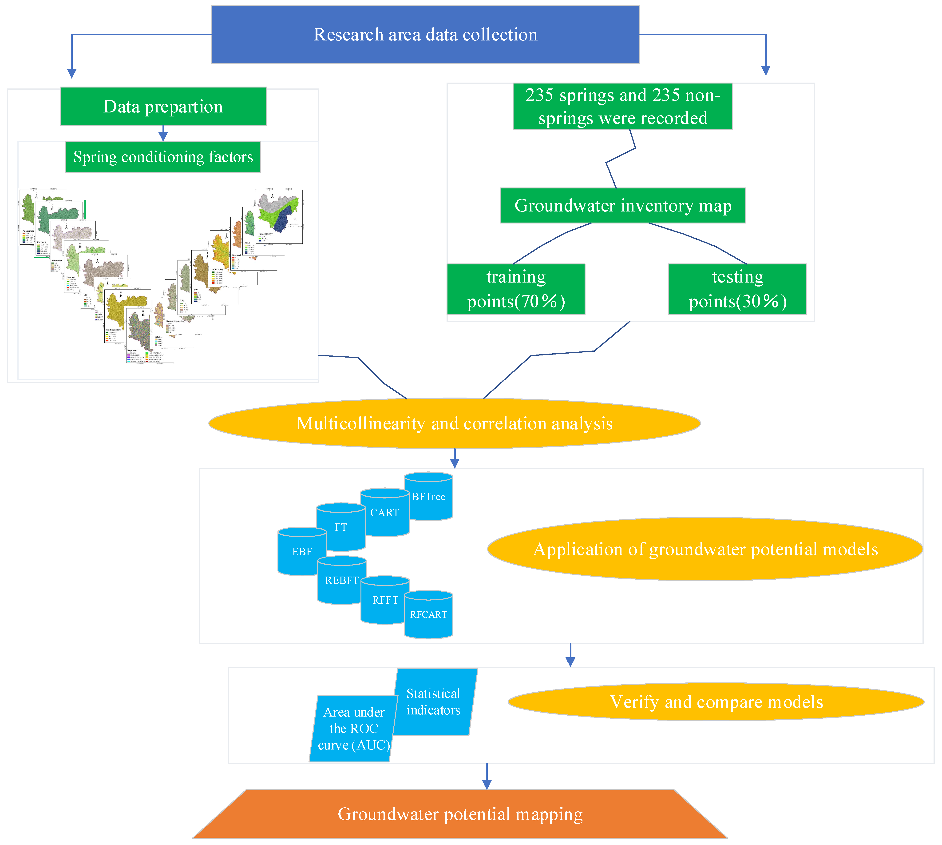
2. Materials and Methods

2.1. Study Area

Wuqi County is located in the Shaanxi Province, China, between 36°33′33″ N and 37°24′27″ N latitudes and 107°38′57″ E and 108°32′49″ E longitudes (Figure 1). It covers an area of approximately 3791 km2. The topographical elevation of the study area varies between 1230 m and 1800 m above sea level (a.s.l.) [26].
The study area is a hilly and gully region of the Loess Plateau. The rivers in the county belong to the Yellow River system, and the main stream is deep and the tributaries are densely distributed. There are 636 rivers with drainage areas larger than 1 km2, out of which 516 rivers have drainage areas between 1 and 10 km2, 93 rivers have drainage areas between 10 and 50 km2, 33 rivers have drainage areas between 50 and 100 km2, and 10 rivers have drainage areas larger than 100 km2. The total length of rivers is 3255.96 km, and the river network density is 0.86 km/km2.
The Luo River, which is the largest river in the study area, is a secondary tributary of the Yellow River and is the main body of the surface hydrological network in the area. The river network density of drainage areas larger than 1 km2 is 0.9 km/km2. The relative height difference of ravines is 120–567 m, and the average longitudinal gradient of tributaries is between 2.5‰ and 9.13‰.

2.2. Data Processing

In this study, a total of 235 springs and 235 non-springs were recorded by collecting historical groundwater-related data and conducting field investigations. In general, the occurrence and utilization of groundwater are related to various conditioning factors; sixteen conditioning factors were selected in this study, including altitude, plan curvature, profile curvature, curvature, slope angle, slope aspect, stream power index (SPI), topographic wetness index (TWI), stream transport index (STI), normalized difference vegetation index (NDVI), land use, soil, lithology, distance to roads, distance to rivers, and rainfall (Supplementary Figure S1).
Slope angle, slope aspect, plan curvature, profile curvature, curvature, altitude, SPI, TWI, and STI are topographic factors [27]. They can be extracted from a digital elevation model (DEM) with a spatial resolution of 30 m. Lithology and soil are geological factors that can be extracted from geological maps. Distances to roads and distances to rivers are extracted from topographic maps [18]. Rainfall data can be downloaded from the Met Office [28]. NDVI and land use maps are created from enhanced thematic mapper plus (ETM+) images [29], and supervised classification is carried out in ENVI software [30].
Slope angle is the change in surface altitude and is the main factor affecting surface water flow [31]. It controls the recharge of groundwater [32]. Slope angle indirectly affects groundwater conditions by affecting surface runoff velocity and vertical filtration [33]. In this study, the slope map is divided into six categories by the natural fault classification scheme [34]: 0–10°, 10–20°, 20–30°, 30–40°, 40–50°, and >50°.
Slope aspect is one of the most important conditions for the identification of groundwater status. It is divided into 10 direction categories in ArcGIS10.5: flat (−1), north (0–22.5), northeast (22.5–67.5), east (67.5–112.5), southeast (112.5–157.5), south (157.5–202.5), southwest (202.5–247.5), west (247.5–292.5), northwest (292.5–337.5), and north (337.5–360).
Altitude refers to the height of a point relative to the base level, which affects the local conditions of the groundwater distribution area [20]. In this study, DEM was used to generate elevation maps, and the natural breaks method was adopted to redivide elevation maps into six categories: 1230–1300 m, 1300–1400 m, 1400–1500 m, 1500–1600 m, 1600–1700 m, and 1700–1800 m.
Plan curvature is a topographically-based variable that shows the direction in which water flows [21]. There are three types of planar curvature: concave (curvature < 0), convex (curvature > 0), and flat (curvature = 0) [35]. In this study, Plan curvature is divided into the following 5 sections: (−7.49)–(−1.11), (−1.11)–(−0.37), (−0.37)–0.25, 0.25–0.99, 0.99–3.03.
Profile curvature shows the rate at which the slope differs in the direction of the highest slope [18]. In this study, profile curvature is divided into 5 categories: (−10.85)–(−1.57), (−1.57)–(−0.47), (−0.47)–0.37, 0.37–1.47, 1.47–10.66.
Curvature affects the spatial variation of groundwater flow, soil moisture, and other hydrological conditions, which indirectly affect the recharge of groundwater [36]. In this study, the curvature was divided into 5 categories by the natural breaks method: (−15.11)–(−2.31), (−2.31)–(−0.72), (−0.72)–0.52, 0.52–2.00, 2.00–13.78.
Based on a digital model (DEM), TWI mainly evaluates the impact of topographic and soil characteristics on soil water distribution. TWI is a secondary topographic index that can describe the location and size of topographic conditions in the saturated source area of surface runoff [37]. The formula is as follows:
T W I = l n [ S C A t a n β ]
where SCA represents the confluence area on the unit contour length flowing through a point on the surface. β represents the slope gradient of a terrain at a certain elevation. In this study, the natural breaks method is used in ArcGIS10.5 to reclassify TWI into 5 categories: <2, 2–2.5, 2.5–3.
SPI is based on the assumption that the flow rate is relative to a specific catchment area and can be used to measure the erosion capacity of flowing water [18]. It can show potential water erosion at specific locations in the basin [21]. SPI can be defined as:
S P I = A s t a n β
where, A s represents catchment area; β represents slope.
STI is a variable that describes the erosion and deposition processes of water flow [38]. In this study, STI is reclassified into 5 categories: <10, 10–20, 20–30, 30–40, and >40.
NDVI is a remote sensing index that reflects the status of land cover vegetation. [39], and it can affect changes in groundwater level [40] and groundwater flow [41]. NDVI is determined by the sum of the red portion (R) and the formula is as follows:
N D V I = I R R I R + R
This research extracts NDVI from satellite images and reclassifies them into five categories: (−0.17)–0.10, 0.10–0.14, 0.14–0.17, 0.17–0.21, 0.21–0.41.
Due to the hydrological and mechanical characteristics of vegetation, land use has also been regarded as an important factor affecting groundwater potential in many studies [42]. In this study, the land use map is divided into six categories: farm land, forest land, grass land, water bodies, construction land, and bare land.
Soil type and texture will affect runoff characteristics and infiltration groundwater recharge and play an extremely important role in groundwater potential evaluation [43]. In this study, the soil map is divided into 5 categories: sticky black loessial soils (Type A), new soils (Type B), cultivated loessial soils (Type C), red clay soils (Type D), and alluvial soils (Type E).
Lithology can affect hydrogeological characteristics such as hydraulic conductivity, aquifer porosity, and groundwater flow [44]. In this study, lithology maps are divided into four categories: Group A, Group B, Group C, and Group D.
In this study, 5 different buffers were generated in ArcGIS 10.5 at intervals of 50 m: <50 m, 50–100 m, 100–150 m, 150–200 m, and >200 m.
The existence of rivers has a significant impact on the degree of erosion and infiltration [45]. In this study, river buffer zones are divided into 5 types: <50 m, 50–100 m, 100–150 m, 150–200 m, and >200 m.
Rainfall is one of the most important factors in the evaluation of groundwater potential. Rainfall can replenish water in the aquifer [46]. In this study, the rainfall map is divided into three categories: <400 mm/year, 400–450 mm/year, and >450 mm/year.

3. Methodology

There are four main steps in this research (Figure 2): (1) Describe the study area and prepare groundwater potential conditioning factors; (2) use GIS software to extract the main control factors that affect the potential of groundwater and draw related layers; (3) optimize the selected model and select the best parameters for groundwater potential modeling; (4) use a ROC curve to verify the generated groundwater potential map.

3.1. Multicollinearity among Factors

Multicollinearity refers to the phenomenon where two or more impact factors are highly correlated in the regression model [47]. When there is a multicollinear relationship between the selected conditioning factors, the established model will find it difficult to accurately estimate the results. Therefore, the influencing factors with collinearity should be eliminated before modeling. It is generally determined by the variance inflation factor (VIF) and tolerance (TOL) [48,49]. VIF is the reciprocal of TOL [50]. The larger the VIF, the smaller the TOL, indicating that the collinearity is more serious [51].
T O L = 1 - R 2
V I F = 1 T O L

3.2. Evidential Belief Function (EBF)

The Dempster–Shafer theory, also known as belief function and evidence theory [52], is a method of mathematical evidence theory [53]. It was first proposed and introduced by Dempster in 1968, and then further improved and gradually matured by his student Shafer in 1976 [54]. It belongs to the category of artificial intelligence and was first applied to expert systems with the ability to process uncertain information [55].
The EBF model is a bivariate model based on Dempster–Shafer theory [56], which is applied to the spatial correlation evaluation of impact factors and dependent variables, including four equations.
B e l A i j = W A i j ( D ) j = 1 n W A i j ( D )
W A i j ( D ) = N ( T A i j ) / N ( T ) [ N ( A i j ) N ( T A i j ) ] / [ N ( A ) N ( T ) ]
D i s A i j = W A i j ( D ¯ ) j = 1 n W A i j ( D ¯ )
W A i j ( D ¯ ) = [ N ( A i j ) N ( T A i j ) ] / N ( A i j ) [ N ( A ) N ( T ) N ( A i j ) + N ( T A i j ) ] / [ N ( A ) N ( T ) ]
U n c A i j = 1 B e l A i j D i s A i j
P l s A i j = B e l A i j + U n c A i j = 1 D i s A i j
where T represents the dependent variable, Aij represents the jth class of the ith evaluation factor, and A represents the evaluation area; N(T) represents the total number of dependent variables; N(Aij) represents the number of evaluation units in the jth class of the ith evaluation factor; N(TAij) represents the number of dependent variables in the jth class of the ith evaluation factor; and N(A) represents the total number of evaluation units in the evaluation area.
W A i j ( D ) is the ratio of the conditional probability that D exists given the presence of Aij to the conditional probability that D exists given the absence of Aij; W A i j ( D ¯ ) is the ratio of the conditional probability that D does not exist given the presence of Aij to the conditional probability that D does not exist given the absence of Aij.

3.3. Rotation Forest (RF)

Rotating forest is a newly developed classifier ensemble technology based on feature extraction [57]. In RF, every basic cluster is trained by the principal component analysis (PCA) algorithm, and feature F is divided into K subsets. For each subset, the PCA algorithm is used to keep all principal components to avoid the loss of mutation information. The advantage of RF is that it improves the variability of data and the accuracy of clustering [58].
The main steps of establishing an RF model are: (1) randomly dividing the attributes of the training data set into K subsets; (2) sampling these subsets by Bootstrap and carrying out principal components on each subset; (3) reset the rotation matrix and train the classifier based on the rotation data set; (4) combining the results of the trained classifiers to output the final class label; and (5) assigning these class labels to each pixel. Finally, a groundwater potential map is generated in the ArcGIS environment.

3.4. Best-First Decision Tree Classifier (BFTree)

EFTree is a decision tree based on a learning algorithm. It uses multiple classifiers to create a classification that can optimize the result and make it better than a model with only one classifier [59]. The best-first decision tree finds the split that leads to maximal information gain, or Gini gain, in every splitting process [60] and stops growing trees when all instances belong to a single value, when the best information gain is not greater than zero, or when it grows to the specified number. The best-first decision tree shows good classification performance.

3.5. Classification and Regression Tree (CART)

The CART model is a binary recursive partition proposed by Breiman et al. [61]. It can deal with continuous and nominal attributes as targets and predictive indicators. It has the ability to resist missing data, and its variables do not need to have a normal distribution [62]. CART is a binary tree structure based on a decision tree. The CART builds classification trees for categorical predictor variables and regression trees for predicting continuous dependent variables [63]. There are two main ideas for establishing a classification regression tree: (1) For each predictor, all possible binary splits of the predictor values are considered, and the best split of each predictor is found. (2) Comparing each predictor by reduction of heterogeneity and finding the best split overall with the largest reduction. Repeat the two-step procedure until there is no meaningful reduction of the response variable and the CART is finished.

3.6. Functional Trees (FT)

FT is a multi-classification model using a tree model for learning that can be used for both regression and classification problems [64]. The main feature of the FT model is that the logistic regression function is used to segment the nodes in the function and predict the function leaves instead of separating inputs at tree nodes by comparing the values of input features with uniform values [65]. The accuracy of the FT model is usually related to the minimum number of instances per leaf of the bootstrap iteration and the function tree [64]. The main difference between FT and other hierarchical models is that instead of dividing inputs by comparing the values of input attributes with a constant on tree nodes, it uses logistic regression functions on functional nodes to divide them and make predictions on functional leaves [65].

3.7. Performance Evaluation of Models

The validation of the results of the established model is one of the most important tasks in groundwater potential mapping. Without verification, the prediction model has no scientific significance [66]. In this study, the predictive ability of the model was evaluated through statistical indicators and the receiver operating characteristic curve (ROC) [67]. The ROC curve is a comprehensive indicator reflecting the sensitivity and specificity of continuous variables; each point on the curve reflects the susceptibility to the same signal stimulus. The abscissa of the ROC curve is 1-specificity, also known as the false positive rate, expressed by FPR, and the ordinate is sensitivity, also known as the true positive rate, expressed by TPR. Generally, the area under the ROC curve (AUC) can be used to evaluate the performance of the model [68,69]. The AUC is defined as the area under the ROC curve, with a value ranging from 0.5 to 1. It can intuitively describe the difference in model performance, and the closer the AUC value is to 1, the higher the accuracy of the corresponding model and the more realistic and reliable the prediction results [70]. The ROC curve index can be calculated using the following formula:
S e n s i t i v i t y = T P T P + F N
S p e c i f i c i t y = T N T N + F P
A c c u r a c y = T P T P + T N + F P + F N
T S S = S e n s i t i v i t y + S p e c i f i c i t y 1
M C C = T P × T N - F P × F N ( T P + F P ) ( T P + F N ) ( T N + F P ) ( T N + F N )
F - S c o r e = 2 × p r e c i s i o n × r e c a l l / ( p r e c i s i o n + R e c a l l )
where TP (true positive) and TN (true negative) are the number of pixels that are accurately classified and FP (false positive) and FN (false negative) are the number of pixels that are inaccurately classified.
TSS is true skill statistics; it is an index that measures the ability of predicted values to distinguish between events and non-events through all elements in the confusion matrix [71].
MCC is the Matthews correlation coefficient; it is a measure of binary classification [72]. The metric is the correlation coefficient between the actual and predicted classes. MCC = 1, thinking the final result is a perfect prediction; MCC = 0, representing a complete divergence between random prediction and observation; M C C = - 1 , which represents a complete divergence between prediction and observation [73].
The F-Score is mainly used to evaluate the accuracy of the two-class model.
This study also used the chi-square test to evaluate the degree of deviation between the observed value and the theoretical value in the model [74]. The chi-square value is proportional to the degree of deviation.
In addition, this study also evaluated the significance of the results by calculating the p value. p value is a parameter used to determine the result of a hypothesis test. Generally, whether the result is significant is judged by the significance level α . In this study, the 95% confidence interval is selected, and the significance level α = 0.05 is used. If p > 0.05, the result is not significant; if p < 0.05, the result is significant.

4. Results

4.1. Correlation Analysis

The results of the multicollinearity analysis in this study are shown in Figure 3. As can be seen from the above figure, among the 16 groundwater conditioning factors, the highest VIF value is 1.625 and the lowest TOL value is 0.615, indicating that there is no multicollinearity among the sixteen conditioning factors.
Subsequently, the importance of each impact factor is calculated based on the ReliefF method [75]. The algorithm can handle multi-class problems and regression problems where the target attribute is a continuous value [76]. ReliefF method results show that distance to rivers has the greatest impact on groundwater potential (AM = 0.099), while curvature has the smallest influence on groundwater potential (AM = 0.006) (Figure 4).
Based on the EBF model, this study analyzed the correlation between groundwater and conditioning factors (Supplementary Figure S2). Among them, the Bel value reflects the relationship between groundwater influencing factors and the groundwater level, and the Bel value is directly proportional to the groundwater level. The greater the Bel value, the greater the impact on groundwater potential.
For the plan curvature, in the (0.25–0.99) level, the Bel value is the largest (0.251), followed by the (−1.11)–(−0.37) level, where the Bel value is 0.223. From the perspective of profile curvature, the Bel value of 0.37–1.47 is the largest (0.294). Regarding curvature, in the categories (0.52–2.00) and (−2.31)–(−0.72), the Bel value is the largest, 0.247 and 0.242, respectively. In terms of slope angle, the slope angle is between (0–10°), and the Bel value is the largest (0.327), followed by the slope angle between (10–20°), and the Bel value is 0.271. This shows that the slope range (0–20°) has the greatest impact on groundwater potential. The slope bel = 0 greater than 40° has no effect on the groundwater potential. In terms of slope aspect, the north slope (Bel = 0.231) and the east slope (Bel = 0.180) have a greater impact on the potential of groundwater, with the least impact in the flat direction (Bel = 0). In the altitude range (1230–1500 m), the Bel value increases with the increase in altitude, and when the Bel value reaches its maximum at 1400–1500 m, then the Bel value decreases as the altitude increases. When the altitude increases to 1700–1800 m, the Bel decreases to 0. The range of SPI is (60–80) and (>80), and the Bel value is 0.254 and 0.239, respectively. It shows that the stronger the erosion ability of flowing water, the greater the impact on groundwater potential. In the range of (>3.5) and (3–3.5), the Bel value is the largest, at 0.339 and 0.256, respectively. Shows that the greater the recharge of the groundwater aquifer, the greater the impact on groundwater potential. STI is in the range (<10), and the Bel value is the largest (Bel = 0.271). NDVI is in the range of (−0.17)–(0.10), and the Bel value is the largest (Bel = 0.290). It shows that the NDVI value is in the range of (−0.17)–(0.10), which will have a greater impact on the potential of groundwater. In terms of land use, the Bel value of the forest land category is the largest (Bel = 0.523). When the soil type is B, the Bel value is the largest (Bel = 0.646). In soil type D, Bel = 0, indicating that this type has little effect on groundwater potential. In GroupD, the lithology has the largest Bel value (Bel = 0.400), followed by GroupB, with a Bel value of 0.318. This is because the lithology and hydrological characteristics of this group are poor, which has a greater impact on the flow characteristics of groundwater and the porosity and permeability of the aquifer. Therefore, it has a greater impact on groundwater potential. The Bel value of GroupC lithology is 0, indicating that the lithology of this group has almost no effect on the potential of groundwater. For road distance within the range of (<50 m) and (50–100 m), the Bel value is the largest, 0.427 and 0.339, respectively. This is because the road affects the diving of groundwater and the capillary water rising from the upper stagnant surface. The distance to the river is within the range of 50–100 m, and the Bel value is the largest (Bel = 0.390). As rivers increase the recharge and infiltration of groundwater, the further away from the river, the lower the potential of groundwater. Rainfall is a crucial factor because it will directly affect the hydrological characteristics of groundwater, such as runoff and recharge. Its three categories all have large Bel values. Among them, the rainfall is within the medium level range of 400–450 mm/year, and the Bel value is the largest (Bel = 0.491), indicating that medium rainfall is more conducive to groundwater recharge.

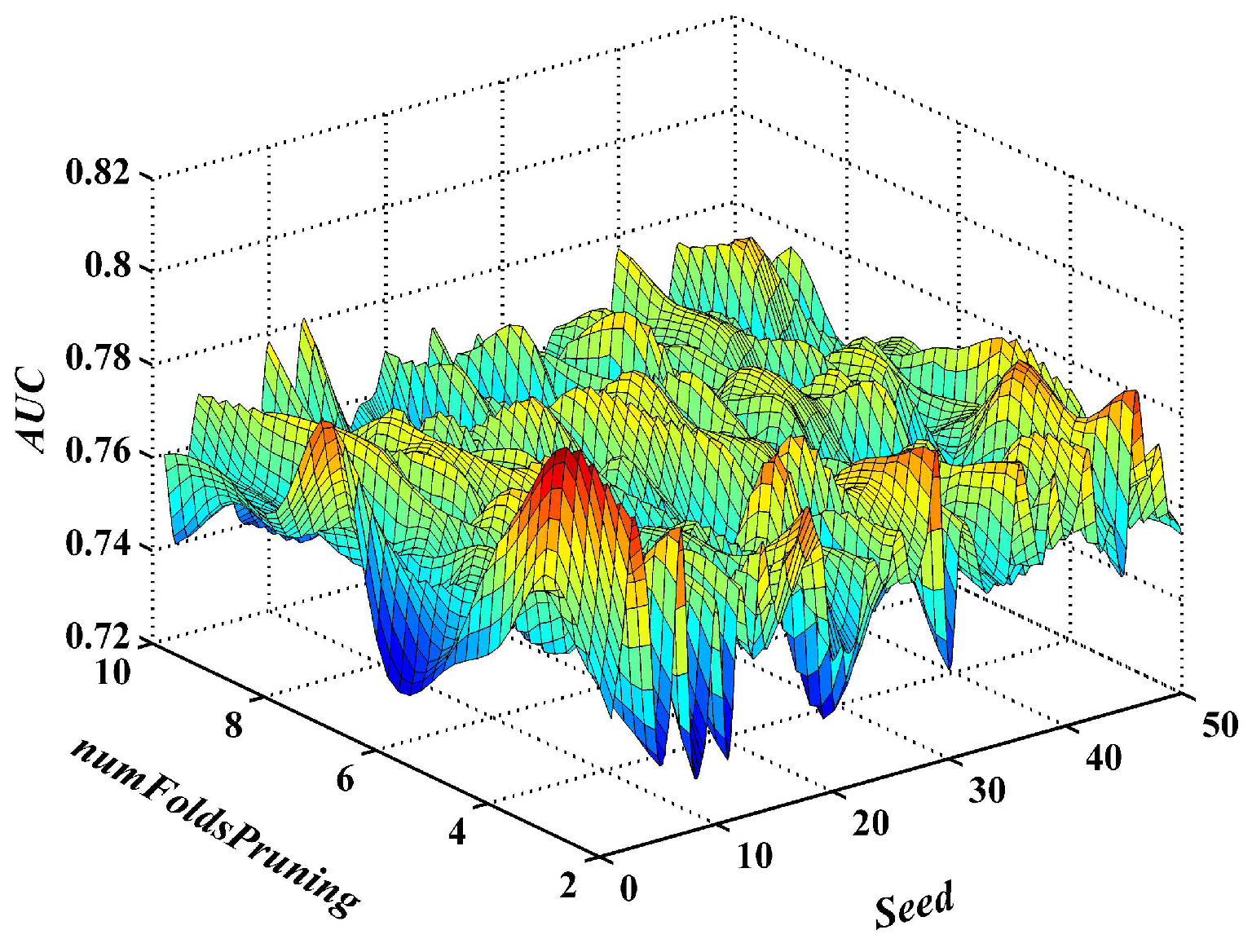
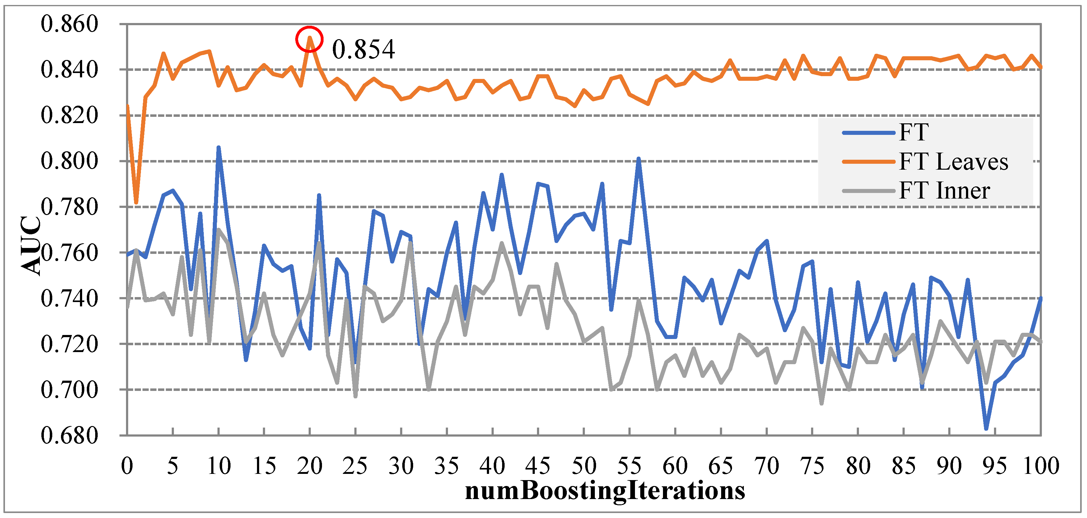
4.2. Configuration and Training of the Models

Groundwater potential mapping models were constructed using the Weka and Matlab platforms. In the training process of the BFT model, the optimal value of the parameters is found through the heuristic test using the training data set, and the groundwater potential model is established. In this process, the BFT model selects post-pruning and pre-pruning as pruning strategies and then adjusts seed and numFoldsPruning, where seed represents the random number seed to be used and numFoldsPruning represents the number of folds for internal cross-validation.
Finally, import all seed values, numFoldsPruning values, and corresponding AUC values into Matlab software to establish the optimized surface of the BFT model (Figure 5a).
The CART model is also optimized by adjusting the parameters of seed and numFoldsPruning, and its optimized surface is shown in Figure 6.
There are three types of FT models: FT, FTLeaves, and FTInner. All model types require tuning of the parameter numboostingiteration (numBoostingIteration represents setting a fixed number of iterations for LogitBoost). Record the AUC values corresponding to each parameter on the curve. The optimization curves corresponding to these three model types are shown in Figure 7.
For hybrid models, the optimal parameters of the base models are first found, and then the relevant parameters (seed and number of iterations) of the ensemble models are adjusted. NumIterations represents the number of iterations to perform. Finally, draw the optimized surface of each ensemble model according to the optimization parameters calculated by Weka software (Figure 8). The optimized parameters of all selected models are shown in Table 1.

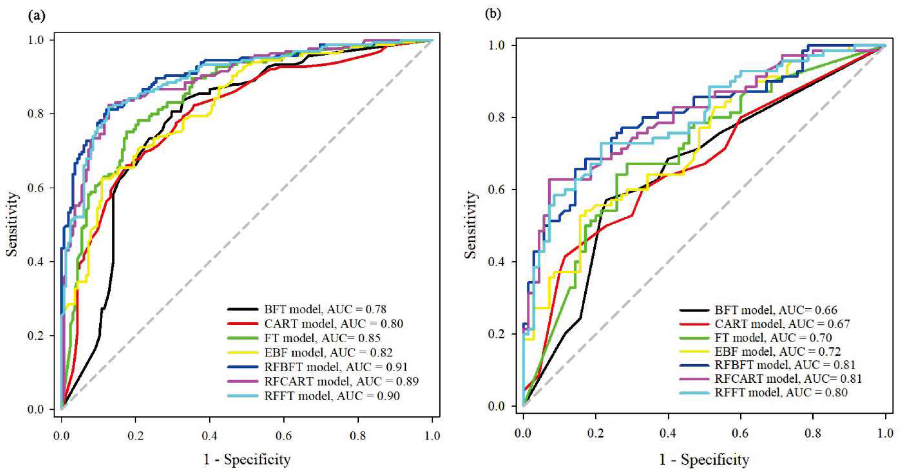
4.3. Model Performance and Validation

Performance of models using cutoff-dependent metrics (Supplementary Table S1). The training data of the RFCART model has the highest MCC value (0.679), indicating that in the training data set, the correlation coefficient between the actual category and the predicted category of the model is the largest and the correlation is the highest. Its TSS value is also the largest (0.678), which shows that in the training data set, the fit between the actual groundwater level and the predicted groundwater level is excellent. In addition, the accuracy value and F-score value of the training data of the RF-CARF model are higher than those of other models.
Validation of models using cutoff-dependent metrics (Supplementary Table S2). In this table, the accuracy, F-Score, and TSS values of the validation data sets of the RF-BFT and RF-FT models are more obvious. The MCC value of the validation data of the RF-BFT model is the largest (0.489), which shows that in the validation data set, the correlation between the actual and predicted classes of this model is more consistent.
Parameters of ROC curves with a training dataset (Table 2): It can be seen that in the training data set, all seven models have good predictive capabilities. Among them, the RF-BFT model has the highest AUC value (0.911), followed by the RF-FT model and the RF-CART model, at 0.898 and 0.894, respectively. In addition, Table 3 also describes the standard errors (SE) of these 7 models and the upper and lower limits of the asymptotic 95% confidence interval. These results all show an error value within the normal range. The p values in Table 3 are all <0.0001, indicating that the result is significant.
Parameters of ROC curves with testing datasets (Table 3): In this table, the result of the validation data set shows that the RF-CART model has the largest AUC value (0.808), followed by the RF-BFT and RF-FT, 0.807 and 0.800, respectively. Shows that the RF-CART model has excellent predictive performance. This is the same result as the training data set.

4.4. Comparison of the Hybrid Model with Benchmark Models

The chi-square test and p value can determine the statistical significance between models [77]. Therefore, this study uses the chi-square value and p value to compare the significant difference in performance between the hybrid model and the benchmark model.
Under the condition of significance level α = 0.05 , the larger the chi-square value and the corresponding p value is less than 0.05, indicating that the model performance is significantly different. It can be seen that there are significant differences in the performance of all models (Table 4).

4.5. Generation of Groundwater Potential Maps

After training and testing procedures in this study, groundwater potential maps of these 7 models were obtained, and four different classification methods were used to reclassify the obtained GPM into 5 categories: very low (VLC), low (LC), moderate (MC), high (HC), and very high (VHC). The four classification methods are: geometric interval, natural breaks, quantile, and equal interval [78]. Figure 9a shows the spatial distribution and proportion of each potential class of each model under these four classification methods. It can be seen from the figure that in the high potential category, groundwater is more distributed, and all models have similar spatial distributions. In order to select the optimal classification method, this study uses the five potential classes as the abscissa and the groundwater point density (GSD) as the ordinate to draw the point density line graphs of these four classification methods (Figure 10). The point density line chart can intuitively reflect the distribution proportions of the five potential classes under different models. It can be seen from the figure that in the natural breaks classification method, the higher the potential category, the larger the GSD value, and the more groundwater distribution. Furthermore, the natural break method has the best classification performance, among which the results of the RF-BFT model are the most reliable. Therefore, this study uses the natural breaks method to reclassify the groundwater potential map.
The histogram of the spatial distribution of the five potential classes of each model obtained using the natural break method is shown in Supplementary Figure S3b. In this figure, the five potential classes of the RFBFT, RF-ART, and RFFT ensemble models have similar spatial distributions. The pixel percentage decreases with the increase in the potential category, and the percentage of groundwater distribution increases with the increase in the potential category. This rule is confirmed in other articles [79]. The EBF model shows different results: The pixel percentage in the LC and MC categories is larger, while the pixel percentage in the VLC category is relatively small.
This study uses the natural breaks method to generate the final groundwater potential maps of seven models (Figure 11). It can be seen from the figure that the very high (VHC) groundwater level area in Wuqi is mainly distributed in the eastern and western valleys with lower altitude, and the distribution ratio is consistent with the above results, which also shows that the classification selected in this paper is appropriate.

5. Discussion

This article uses the BFT model, CART model, and FT model as the base classifiers to integrate the rotation forest model with them to model the distribution of groundwater in Wuqi County, China. In addition, the area under the receiver operating characteristic curve (AUC) is used to verify the accuracy and success rate of the training and test data. The results show that the AUC values of the ensemble model are all greater than those of the benchmark model. The articles of Nguyen et al. [80], Razavi-Termeh [22] and Lee and Oh [81] also have relevant instructions for sub-model integration. In the report of Hosseinalizadeh et al. [82], they integrated Bag, RS, and RF methods with the BFT model, respectively. The final training and verification results show that the AUC value of the BFT single model is the smallest. In addition, some researchers have also tried to combine different base models. Pham [20] integrated three different hybrid computing intelligent models with basic decision stump classifiers to draw groundwater potential maps. Kordestani [21] implemented the evidence belief function and the enhanced regression tree (EBF-BRT) ensemble algorithm in groundwater potential mapping. Although the ensemble methods used by the researchers are different, the final results all explain that the correct combination of weak classifiers can effectively solve the overfitting problem in the modeling process, thereby improving the performance of the model. This also confirms that the conclusions of this study are true and accurate. The rotation forest algorithm used in this study has obtained good application results in some studies [83]. However, Naghibi et al. [15] have obtained different results. The scholar used the EBFTM data mining method as a new integrated model and compared it with the tree-based rotation forest model to establish a groundwater potential map. It was found that the results obtained by the EBFTM method were even better. The reason for the different research results in this literature may be due to the differences in the characteristics of the data samples and the research objects in the selected study area. Therefore, in future research, researchers should choose the corresponding integration method according to the different research areas and apply the selected method to more than two research areas as much as possible, so as to better judge the applicability of the model.
Compared with other studies on groundwater potential, in order to obtain more reliable modeling results, this article also uses the Weka platform to optimize the modeling parameters of the study area and uses a 10-fold cross-validation method to process the sample data. In the study of Naghibi et al. [15], the training data prediction rate of the CART model is only 0.7870. The research results of Nguyen et al. [84] show that the AUC values obtained by the RFBFT model after training and verification are 0.891 and 0.826, respectively. In the report of Pham et al. [64], the AUC value of the FT model training sample is 0.849. However, Zhao and Chen [85] optimized the parameters of one of the models (the LMT model) in the study and finally found that the AUC values of the remaining models that did not participate in the optimization were lower than the LMT model (for example, the AUC values of the RFFT model training and validation data sets are 0.839 and 0.740, respectively). By comparing the reports of these researchers, it can be seen that it is necessary and effective to optimize the parameters of the selected model. However, in the research of Yariyan et al. [86] and Chen et al. [87], the BFT model obtained a better AUC value than this paper without optimization. The reason for this result may be that the climate and hydrological characteristics of the study area are different, which makes the BFT model less applicable to the study area.
Different classification methods produce different results for groundwater potential maps. In this study, four different classification systems (natural break method, quantile, geometric interval, and equal interval) were selected to partition groundwater potential mapping. The reclassification results indicate that the natural break method is the most effective. Baeza et al. [88] also used different methods (equal interval, natural break method, quantile, and standard deviation) to classify landslide sensitivity mapping. The final result demonstrates that the natural break method is the most suitable classification method. Youssef et al. [89] applied the same classification method as this study to partition the landslide sensitivity map, and results illustrate that the quantile method is the most accurate distribution classifier. The initial guess as to the reason for this phenomenon is that the model chosen by the scholar is different from this article. Furthermore, the study area of the report is a basin, while this study area is the Loess Plateau. The difference in the geomorphic units of the study area makes the classification method applicable to different degrees.
This study judged the weight of the selected conditioning factor classes based on the EBF model. When the slope is small, the surface runoff velocity is large, and the impact on the groundwater potential is more obvious. In the research of Ozdemir [90], Naghibi and Pourghasemi [91], the correlation analysis between slope and groundwater potential yielded the same result. Abd Manap et al. [92] believe that altitude has a moderate impact on groundwater potential. According to the study of Tien Bui [33], the larger the SPI value, the greater the impact on the hydrological characteristics of groundwater. Zabihi [35] and Pham [20] believe that the greater the TWI value, the greater the recharge of groundwater aquifers. Chen et al. [13] proposed that the smaller the NDVI value, the easier it is for surface water to penetrate into the ground. The research results of these scholars are basically consistent with this research. However, the STI indicator expressed unexpected results; Kordestani [21] proposed that areas with higher STI values have higher groundwater potential because of the higher groundwater level. This difference may be due to the inconsistency of the impact factor with the geographical characteristics and groundwater generation mechanisms of this study area.
In summary, this study integrates BFTree, CART, FT and RF models, and uses BFTree, CART, FT, RF-BFT, RF-CART, RF-FT, and EBF benchmark models to map groundwater potential in Wuqi County, China. According to the multicollinearity analysis results, the sixteen conditioning factors were not highly correlated. The ReliefF method was used to calculate the importance of each influence factor. The results show that the distance from the river has the greatest influence on the groundwater potential, while the curvature has the least influence on the groundwater potential. Based on the EBF model, we could conclude that all factors contributed to groundwater potential modeling. Finally, use statistical indicators and the ROC curve to verify the accuracy of the model results. The results show that the AUC value of the ensemble model is greater than that of the benchmark model, its prediction rate is higher, and its performance is better. Among them, the RF-BFT model has the highest prediction rate. In summary, the research results obtained in this paper could provide certain reference guidelines for the rational utilization of groundwater resources, ecological environment protection, and regional land planning.

6. Concluding Remarks

Accurate assessment and analysis of the groundwater potential play a pivotal role in groundwater management, development, and utilization. This study uses a decision tree algorithm based on a rotating forest to model the groundwater space in Wuqi County, China. First, sixteen conditioning factors were selected in the study area. Secondly, analyze the collinearity and correlation between the impact factor and groundwater and optimize the various parameters of the selected model. After that, use the BFTree, CART, EBF, and FT models and the RF-BFT, RF-CART, and RF-FT ensemble models to model the groundwater in Wuqi County. Finally, use statistical indicators and the ROC curve to verify the accuracy of the model results. The results show that the AUC value of the ensemble model is greater than the benchmark model, its prediction rate is higher, and the performance is better [93]. Among them, the RF-BFT model has the highest prediction rate. This study also reclassified the groundwater potential map obtained by different classification methods and chose the best classification method to generate the final groundwater potential map of the study area. After comparative analysis, the groundwater potential map results of this study are reliable and can be used as a useful tool for the local government of Wuqi County to explore and develop groundwater potential.

Supplementary Materials

The following supporting information can be downloaded at https://www.mdpi.com/article/10.3390/w15122287/s1, Figure S1: Spring conditioning factors; Figure S2: Conditioning factor histogram based on EBF; Figure S3: Selection of the best classification method for groundwater potential map: (a) geometrical interval, (b) natural breaks, (c) quantile, (d) equal interval; Table S1: Performance of models using cutoff-dependent metrics; Table S2: Validation of models using cutoff-dependent metrics.

Author Contributions

Conceptualization, W.C. and Z.W.; methodology, Z.W., G.W. and W.C.; software, B.L., S.L. and W.X.; validation, Z.W., G.W. and W.C.; formal analysis, Z.W.; investigation, G.W. and W.C.; writing—original draft preparation, Z.W., P.T. and I.I.; writing—review and editing, W.C., Z.N., P.T. and I.I. All authors have read and agreed to the published version of the manuscript.

Funding

This study is supported by the National Natural Science Foundation of China (Grant No. 41807192), the Natural Science Basic Research Program of Shaanxi (Program No. 2019JLM-7), and the Shaanxi Key Research Programme on the QINCHUANGYUAN Scientist and Engineer Project (No. 2023KXJ-134).

Data Availability Statement

Not applicable.

Acknowledgments

The authors wish to express their sincere thanks to Zhao Duan and Xinjian Chen for the useful information provided.

Conflicts of Interest

The authors declare no conflict of interest.

References

  1. Saha, A.; Pal, S.C.; Chowdhuri, I.; Roy, P.; Chakrabortty, R. Effect of hydrogeochemical behavior on groundwater resources in Holocene aquifers of moribund Ganges Delta, India: Infusing data-driven algorithms. Environ. Pollut. 2022, 314, 120203. [Google Scholar] [CrossRef] [PubMed]
  2. Ruidas, D.; Saha, A.; Chowdhuri, I.; Pal, S.C.; Islam, A.T. Application of novel data-mining technique based nitrate concentration susceptibility prediction approach for coastal aquifers in India. J. Clean. Prod. 2022, 346, 131205. [Google Scholar]
  3. He, S.; Wu, J. Hydrogeochemical Characteristics, Groundwater Quality, and Health Risks from Hexavalent Chromium and Nitrate in Groundwater of Huanhe Formation in Wuqi County, Northwest China. Expo. Health 2019, 11, 125–137. [Google Scholar] [CrossRef]
  4. Ruidas, D.; Pal, S.C.; Islam, A.R.M.T.; Saha, A. Characterization of groundwater potential zones in water-scarce hardrock regions using data driven model. Environ. Earth Sci. 2021, 80, 809. [Google Scholar] [CrossRef]
  5. Jaydhar, A.K.; Chandra Pal, S.; Saha, A.; Islam, A.R.M.T.; Ruidas, D. Hydrogeochemical evaluation and corresponding health risk from elevated arsenic and fluoride contamination in recurrent coastal multi-aquifers of eastern India. J. Clean. Prod. 2022, 369, 133150. [Google Scholar] [CrossRef]
  6. He, X.; Wu, J.; He, S. Hydrochemical characteristics and quality evaluation of groundwater in terms of health risks in Luohe aquifer in Wuqi County of the Chinese Loess Plateau, northwest China. Hum. Ecol. Risk Assess. 2019, 25, 32–51. [Google Scholar] [CrossRef]
  7. He, X.; Li, P. Surface Water Pollution in the Middle Chinese Loess Plateau with Special Focus on Hexavalent Chromium (Cr6+): Occurrence, Sources and Health Risks. Expo. Health 2020, 12, 385–401. [Google Scholar] [CrossRef]
  8. Tian, R.; Wu, J. Groundwater quality appraisal by improved set pair analysis with game theory weightage and health risk estimation of contaminants for Xuecha drinking water source in a loess area in Northwest China. Hum. Ecol. Risk Assess. 2019, 25, 132–157. [Google Scholar] [CrossRef]
  9. Das, B.; Pal, S.C.; Malik, S.; Chakrabortty, R. Modeling groundwater potential zones of Puruliya district, West Bengal, India using remote sensing and GIS techniques. Geol. Ecol. Landsc. 2019, 3, 223–237. [Google Scholar] [CrossRef] [Green Version]
  10. Chowdhury, A.; Jha, M.; Chowdary, V.; Mal, B. Integrated remote sensing and GIS-based approach for assessing groundwater potential in West Medinipur district, West Bengal, India. Int. J. Remote Sens. 2009, 30, 231–250. [Google Scholar] [CrossRef]
  11. Kumar, V.A.; Mondal, N.; Ahmed, S. Identification of groundwater potential zones using RS, GIS and AHP techniques: A case study in a part of Deccan volcanic province (DVP), Maharashtra, India. J. Indian Soc. Remote Sens. 2020, 48, 497–511. [Google Scholar] [CrossRef]
  12. Das, S. Comparison among influencing factor, frequency ratio, and analytical hierarchy process techniques for groundwater potential zonation in Vaitarna basin, Maharashtra, India. Groundw. Sustain. Dev. 2019, 8, 617–629. [Google Scholar] [CrossRef]
  13. Chen, W.; Li, H.; Hou, E.; Wang, S.; Wang, G.; Panahi, M.; Li, T.; Peng, T.; Guo, C.; Niu, C.; et al. GIS-based groundwater potential analysis using novel ensemble weights-of-evidence with logistic regression and functional tree models. Sci. Total Environ. 2018, 634, 853–867. [Google Scholar] [CrossRef] [PubMed] [Green Version]
  14. Golkarian, A.; Naghibi, S.A.; Kalantar, B.; Pradhan, B. Groundwater potential mapping using C5. 0, random forest, and multivariate adaptive regression spline models in GIS. Environ. Monit. Assess. 2018, 190, 149. [Google Scholar] [CrossRef] [PubMed]
  15. Naghibi, S.A.; Pourghasemi, H.R.; Dixon, B. GIS-based groundwater potential mapping using boosted regression tree, classification and regression tree, and random forest machine learning models in Iran. Environ. Monit. Assess. 2016, 188, 44. [Google Scholar] [CrossRef]
  16. Mahato, S.; Pal, S. Groundwater potential mapping in a rural river basin by union (OR) and intersection (AND) of four multi-criteria decision-making models. Nat. Resour. Res. 2019, 28, 523–545. [Google Scholar] [CrossRef]
  17. Zeinivand, H.; Ghorbani Nejad, S. Application of GIS-based data-driven models for groundwater potential mapping in Kuhdasht region of Iran. Geocarto Int. 2018, 33, 651–666. [Google Scholar] [CrossRef]
  18. Naghibi, S.A.; Ahmadi, K.; Daneshi, A. Application of Support Vector Machine, Random Forest, and Genetic Algorithm Optimized Random Forest Models in Groundwater Potential Mapping. Water Resour. Manag. 2017, 31, 2761–2775. [Google Scholar] [CrossRef]
  19. Lee, S.; Hong, S.-M.; Jung, H.-S. GIS-based groundwater potential mapping using artificial neural network and support vector machine models: The case of Boryeong city in Korea. Geocarto Int. 2018, 33, 847–861. [Google Scholar] [CrossRef]
  20. Pham, B.T.; Jaafari, A.; Prakash, I.; Singh, S.K.; Quoc, N.K.; Bui, D.T. Hybrid computational intelligence models for groundwater potential mapping. Catena 2019, 182, 104101. [Google Scholar] [CrossRef]
  21. Kordestani, M.D.; Naghibi, S.A.; Hashemi, H.; Ahmadi, K.; Kalantar, B.; Pradhan, B. Groundwater potential mapping using a novel data-mining ensemble model. Hydrogeol. J. 2019, 27, 211–224. [Google Scholar] [CrossRef] [Green Version]
  22. Razavi-Termeh, S.V.; Sadeghi-Niaraki, A.; Choi, S.-M. Groundwater potential mapping using an integrated ensemble of three bivariate statistical models with random forest and logistic model tree models. Water 2019, 11, 1596. [Google Scholar] [CrossRef] [Green Version]
  23. Dietterich, T.G. Ensemble methods in machine learning. In International Workshop on Multiple Classifier Systems; Springer: Berlin/Heidelberg, Germany, 2000; pp. 1–15. [Google Scholar]
  24. Ruidas, D.; Pal, S.C.; Towfiqul Islam, A.R.M.; Saha, A. Hydrogeochemical Evaluation of Groundwater Aquifers and Associated Health Hazard Risk Mapping Using Ensemble Data Driven Model in a Water Scares Plateau Region of Eastern India. Expo. Health 2022, 15, 113–131. [Google Scholar] [CrossRef]
  25. Avand, M.; Janizadeh, S.; Tien Bui, D.; Pham, V.H.; Ngo, P.T.T.; Nhu, V.-H. A tree-based intelligence ensemble approach for spatial prediction of potential groundwater. Int. J. Digit. Earth 2020, 13, 1408–1429. [Google Scholar] [CrossRef]
  26. Chen, W.; Zhao, X.; Tsangaratos, P.; Shahabi, H.; Ilia, I.; Xue, W.; Wang, X.; Ahmad, B.B. Evaluating the usage of tree-based ensemble methods in groundwater spring potential mapping. J. Hydrol. 2020, 583, 124602. [Google Scholar] [CrossRef]
  27. He, C.-B. The Method for Collecting Regional Topographic Factors based on Digital Elevation Model (DEM). For. Inventory Plan. 2007, 2, 18–21. [Google Scholar]
  28. Rahmati, O.; Nazari Samani, A.; Mahdavi, M.; Pourghasemi, H.R.; Zeinivand, H. Groundwater potential mapping at Kurdistan region of Iran using analytic hierarchy process and GIS. Arab. J. Geosci. 2015, 8, 7059–7071. [Google Scholar] [CrossRef]
  29. Yue, W.; Xu, J.; Tan, W.; Xu, L. The relationship between land surface temperature and NDVI with remote sensing: Application to Shanghai Landsat 7 ETM+ data. Int. J. Remote Sens. 2007, 28, 3205–3226. [Google Scholar] [CrossRef]
  30. Jusuf, S.K.; Wong, N.H.; Hagen, E.; Anggoro, R.; Hong, Y. The influence of land use on the urban heat island in Singapore. Habitat Int. 2007, 31, 232–242. [Google Scholar] [CrossRef]
  31. Ettazarini, S. Groundwater potentiality index: A strategically conceived tool for water research in fractured aquifers. Environ. Geol. 2007, 52, 477–487. [Google Scholar] [CrossRef]
  32. Ettazarini, S.; El Mahmouhi, N. Vulnerability mapping of the Turonian limestone aquifer in the Phosphates Plateau (Morocco). Environ. Geol. 2004, 46, 113–117. [Google Scholar] [CrossRef]
  33. Tien Bui, D.; Shirzadi, A.; Chapi, K.; Shahabi, H.; Pradhan, B.; Pham, B.T.; Singh, V.P.; Chen, W.; Khosravi, K.; Bin Ahmad, B. A hybrid computational intelligence approach to groundwater spring potential mapping. Water 2019, 11, 2013. [Google Scholar] [CrossRef] [Green Version]
  34. Bui, D.T.; Pradhan, B.; Lofman, O.; Revhaug, I.; Dick, O.B. Landslide susceptibility assessment in the Hoa Binh province of Vietnam: A comparison of the Levenberg–Marquardt and Bayesian regularized neural networks. Geomorphology 2012, 171, 12–29. [Google Scholar]
  35. Zabihi, M.; Pourghasemi, H.R.; Pourtaghi, Z.S.; Behzadfar, M. GIS-based multivariate adaptive regression spline and random forest models for groundwater potential mapping in Iran. Environ. Earth Sci. 2016, 75, 665. [Google Scholar] [CrossRef]
  36. Dar, I.A.; Sankar, K.; Dar, M.A. Remote sensing technology and geographic information system modeling: An integrated approach towards the mapping of groundwater potential zones in Hardrock terrain, Mamundiyar basin. J. Hydrol. 2010, 394, 285–295. [Google Scholar] [CrossRef]
  37. Razandi, Y.; Pourghasemi, H.R.; Neisani, N.S.; Rahmati, O. Application of analytical hierarchy process, frequency ratio, and certainty factor models for groundwater potential mapping using GIS. Earth Sci. Inform. 2015, 8, 867–883. [Google Scholar] [CrossRef]
  38. Conforti, M.; Robustelli, G.; Luca, F. Comparison of GIS-based gullying susceptibility mapping using bivariate and multivariate statistics: Northern Calabria South Italy. Geomorphology 2011, 134, 297–308. [Google Scholar]
  39. Bischof, R.; Loe, L.E.; Meisingset, E.L.; Zimmermann, B.; Van Moorter, B.; Mysterud, A. A migratory northern ungulate in the pursuit of spring: Jumping or surfing the green wave? Am. Nat. 2012, 180, 407–424. [Google Scholar] [CrossRef] [Green Version]
  40. Aguilar, C.; Zinnert, J.C.; Polo, M.a.J.; Young, D.R. NDVI as an indicator for changes in water availability to woody vegetation. Ecol. Indic. 2012, 23, 290–300. [Google Scholar] [CrossRef]
  41. Petus, C.; Lewis, M.; White, D. Using MODIS Normalized Difference Vegetation Index to monitor seasonal and inter-annual dynamics of wetland vegetation in the Great Artesian Basin: A baseline for assessment of future changes in a unique ecosystem. Int. Arch. Photogramm. Remote Sens. Spatial Inf. Sci. 2012, XXXIX–B8, 187–192. [Google Scholar] [CrossRef] [Green Version]
  42. Davoudi Moghaddam, D.; Rahmati, O.; Haghizadeh, A.; Kalantari, Z. A Modeling Comparison of Groundwater Potential Mapping in a Mountain Bedrock Aquifer: QUEST, GARP, and RF Models. Water 2020, 12, 679. [Google Scholar] [CrossRef] [Green Version]
  43. Termeh, S.V.R.; Khosravi, K.; Sartaj, M.; Keesstra, S.D.; Tsai, F.T.-C.; Dijksma, R.; Pham, B.T. Optimization of an adaptive neuro-fuzzy inference system for groundwater potential mapping. Hydrogeol. J. 2019, 27, 2511–2534. [Google Scholar] [CrossRef]
  44. Ayazi, M.H.A.; Pirasteh, S.; Pili, A.K.A.; Biswajeet, P.; Nikouravan, B.; Mansor, S.J.D.A. Disasters and risk reduction in groundwater: Zagros Mountain, Southwest Iran using geoinformatics techniques. Disaster Adv. 2010, 3, 51–57. [Google Scholar]
  45. Chen, W.; Panahi, M.; Tsangaratos, P.; Shahabi, H.; Ilia, I.; Panahi, S.; Li, S.; Jaafari, A.; Ahmad, B.B.J.C. Applying population-based evolutionary algorithms and a neuro-fuzzy system for modeling landslide susceptibility. CATENA 2019, 172, 212–231. [Google Scholar] [CrossRef]
  46. Oikonomidis, D.; Dimogianni, S.; Kazakis, N.; Voudouris, K. A GIS/Remote Sensing-based methodology for groundwater potentiality assessment in Tirnavos area, Greece. J. Hydrol. 2015, 525, 197–208. [Google Scholar] [CrossRef]
  47. Ruidas, D.; Chakrabortty, R.; Islam, A.R.M.T.; Saha, A.; Pal, S.C. A novel hybrid of meta-optimization approach for flash flood-susceptibility assessment in a monsoon-dominated watershed, Eastern India. Environ. Earth Sci. 2022, 81, 145. [Google Scholar] [CrossRef]
  48. Ruidas, D.; Saha, A.; Islam, A.R.M.T.; Costache, R.; Pal, S.C. Development of geo-environmental factors controlled flash flood hazard map for emergency relief operation in complex hydro-geomorphic environment of tropical river, India. Environ. Sci. Pollut. Res. 2022, 1–16. [Google Scholar] [CrossRef]
  49. Ruidas, D.; Pal, S.C.; Saha, A.; Chowdhuri, I.; Shit, M. Hydrogeochemical characterization based water resources vulnerability assessment in India’s first Ramsar site of Chilka lake. Mar. Pollut. Bull. 2022, 184, 114107. [Google Scholar] [CrossRef]
  50. O’Brien, R.M. A Caution Regarding Rules of Thumb for Variance Inflation Factors. Qual. Quant. 2007, 41, 673–690. [Google Scholar] [CrossRef]
  51. Arabameri, A.; Pourghasemi, H.R. Spatial modeling of gully erosion using linear and quadratic discriminant analyses in GIS and R. In Spatial Modeling in GIS and R for Earth and Environmental Sciences; Elsevier: Amsterdam, The Netherlands, 2019; pp. 299–321. [Google Scholar]
  52. Shafer, G. Dempster-shafer theory. Encycl. Artif. Intell. 1992, 1, 330–331. [Google Scholar]
  53. Sentz, K.; Ferson, S. Combination of Evidence in Dempster-Shafer Theory; Sandia National Laboratories Albuquerque Contemporary Pacific: Sandia, Peru, 2002; Volume 4015. [Google Scholar] [CrossRef] [Green Version]
  54. Liu, Q.; Tian, Y.; Kang, B. Derive knowledge of Z-number from the perspective of Dempster–Shafer evidence theory. Eng. Appl. Artif. Intell. 2019, 85, 754–764. [Google Scholar] [CrossRef]
  55. Cortes-Rello, E.; Golshani, F. Uncertain reasoning using the Dempster-Shafer method: An application in forecasting and marketing management. Expert Syst. 1990, 7, 9–18. [Google Scholar] [CrossRef]
  56. Pourghasemi, H.R.; Kerle, N. Random forests and evidential belief function-based landslide susceptibility assessment in Western Mazandaran Province, Iran. Environ. Earth Sci. 2016, 75, 185. [Google Scholar] [CrossRef]
  57. Rodriguez, J.J.; Kuncheva, L.I.; Alonso, C.J. Rotation forest: A new classifier ensemble method. IEEE Trans. Pattern Anal. Mach. Intell. 2006, 28, 1619–1630. [Google Scholar] [CrossRef] [PubMed]
  58. Kuncheva, L.I.; Rodríguez, J.J. In An experimental study on rotation forest ensembles. In Multiple Classifier Systems; Haindl, M., Kittler, J., Roli, F., Eds.; Springer: Berlin/Heidelberg, Germany, 2017; pp. 459–468. [Google Scholar]
  59. Kumar, N.; Reddy, G.; Chatterji, S. Evaluation of best first decision tree on categorical soil survey data for land capability classification. Int. J. Comput. Appl. 2013, 72, 5–8. [Google Scholar] [CrossRef]
  60. Shi, H. Best-First Decision Tree Learning. Master’s Thesis, The University of Waikato, Hamilton, New Zealand, 2007. [Google Scholar]
  61. Breiman, L.; Friedman, J.; Stone, C.J.; Olshen, R.A. Classification and Regression Trees; CRC Press: Boca Raton, FL, USA, 1984. [Google Scholar]
  62. Belgiu, M.; Dragut, L. Random forest in remote sensing: A review of applications and future directions. ISPRS J. Photogramm. Remote Sens. 2016, 114, 24–31. [Google Scholar] [CrossRef]
  63. Chaurasia, V.; Pal, S. Early prediction of heart diseases using data mining techniques. Caribb. J. Sci. Technol. 2013, 1, 208–217. [Google Scholar]
  64. Gama, J. Functional Trees. MLear 2004, 55, 219–250. [Google Scholar] [CrossRef]
  65. Pham, B.T.; Tien Bui, D.; Pourghasemi, H.R.; Indra, P.; Dholakia, M.B. Landslide susceptibility assesssment in the Uttarakhand area (India) using GIS: A comparison study of prediction capability of naïve bayes, multilayer perceptron neural networks, and functional trees methods. Theor. Appl. Climatol. 2017, 128, 255–273. [Google Scholar] [CrossRef]
  66. Chung, C.-J.F.; Fabbri, A.G. Validation of Spatial Prediction Models for Landslide Hazard Mapping. Nat. Hazards 2003, 30, 451–472. [Google Scholar] [CrossRef]
  67. Chen, Q.; Yan, E.; Huang, S.; Wang, Q. Susceptibility evaluation of geological disasters in southern Huanggang based on samples and factor optimization. Bull. Geol. Sci. Technol. 2020, 39, 175–185. [Google Scholar] [CrossRef]
  68. Chen, W.; Shahabi, H.; Shirzadi, A.; Hong, H.; Akgun, A.; Tian, Y.; Liu, J.; Zhu, A.X.; Li, S. Novel hybrid artificial intelligence approach of bivariate statistical-methods-based kernel logistic regression classifier for landslide susceptibility modeling. Bull. Eng. Geol. Environ. 2018, 78, 4397–4419. [Google Scholar] [CrossRef]
  69. Huang, F.; Li, J.; Wang, J.; Mao, D.; Sheng, M. Modelling rules of landslide susceptibility prediction considering the suitability of linear environmental factors and different machine learning models. Bull. Geol. Sci. Technol. 2022, 41, 44–59. [Google Scholar]
  70. Miraki, S.; Zanganeh, S.H.; Chapi, K.; Singh, V.P.; Shirzadi, A.; Shahabi, H.; Pham, B.T. Mapping groundwater potential using a novel hybrid intelligence approach. Water Resour. Manag. 2019, 33, 281–302. [Google Scholar] [CrossRef]
  71. Pourghasemi, H.R.; Kariminejad, N.; Amiri, M.; Edalat, M.; Zarafshar, M.; Blaschke, T.; Cerda, A. Assessing and mapping multi-hazard risk susceptibility using a machine learning technique. Sci. Rep. 2020, 10, 3203. [Google Scholar] [CrossRef] [PubMed] [Green Version]
  72. Matthews, B.W. Comparison of the predicted and observed secondary structure of T4 phage lysozyme. Biochim. Biophys. Acta 1975, 405, 442–451. [Google Scholar] [CrossRef]
  73. Wang, Y.; Fang, Z.; Hong, H. Comparison of convolutional neural networks for landslide susceptibility mapping in Yanshan County, China. Sci. Total Environ. 2019, 666, 975–993. [Google Scholar] [CrossRef]
  74. Sarkar, S.; Kanungo, D. An integrated approach for landslide susceptibility mapping using remote sensing and GIS. Photogramm. Eng. Remote Sens. 2004, 70, 617–625. [Google Scholar] [CrossRef]
  75. Robnik-Šikonja, M.; Kononenko, I. Theoretical and empirical analysis of ReliefF and RReliefF. Mach. Learn. 2003, 53, 23–69. [Google Scholar] [CrossRef] [Green Version]
  76. Kononenko, I.; Robnik-Sikonja, M.; Pompe, U. ReliefF for estimation and discretization of attributes in classification, regression, and ILP problems. Artif. Intell. Methodol. Syst. Appl. 1996, 2, 31–40. [Google Scholar]
  77. Tallarida, R.J.; Murray, R.B. Chi-square test. In Manual of Pharmacologic Calculations; Springer: Berlin/Heidelberg, Germany, 1987; pp. 140–142. [Google Scholar]
  78. Pradhan, B.; Lee, S. Delineation of landslide hazard areas on Penang Island, Malaysia, by using frequency ratio, logistic regression, and artificial neural network models. Environ. Earth Sci. 2010, 60, 1037–1054. [Google Scholar] [CrossRef]
  79. Li, Y.; Chen, W. Landslide Susceptibility Evaluation Using Hybrid Integration of Evidential Belief Function and Machine Learning Techniques. Water 2020, 12, 113. [Google Scholar] [CrossRef] [Green Version]
  80. Nguyen, P.T.; Ha, D.H.; Jaafari, A.; Nguyen, H.D.; Van Phong, T.; Al-Ansari, N.; Prakash, I.; Le, H.V.; Pham, B.T. Groundwater Potential Mapping Combining Artificial Neural Network and Real AdaBoost Ensemble Technique: The DakNong Province Case-study, Vietnam. Int. J. Environ. Res. Public Health 2020, 17, 2473. [Google Scholar] [CrossRef] [PubMed] [Green Version]
  81. Lee, S.; Oh, H.-J. Ensemble-based landslide susceptibility maps in Jinbu area, Korea. In Terrigenous Mass Movements; Springer: Berlin/Heidelberg, Germany, 2012; pp. 193–220. [Google Scholar]
  82. Hosseinalizadeh, M.; Kariminejad, N.; Chen, W.; Pourghasemi, H.R.; Alinejad, M.; Behbahani, A.M.; Tiefenbacher, J.P. Spatial modelling of gully headcuts using UAV data and four best-first decision classifier ensembles (BFTree, Bag-BFTree, RS-BFTree, and RF-BFTree). Geomorphology 2019, 329, 184–193. [Google Scholar] [CrossRef]
  83. Hong, H.; Liu, J.; Bui, D.T.; Pradhan, B.; Acharya, T.D.; Pham, B.T.; Zhu, A.-X.; Chen, W.; Ahmad, B.B. Landslide susceptibility mapping using J48 Decision Tree with AdaBoost, Bagging and Rotation Forest ensembles in the Guangchang area (China). Catena 2018, 163, 399–413. [Google Scholar] [CrossRef]
  84. Nguyen, V.V.; Pham, B.T.; Vu, B.T.; Prakash, I.; Jha, S.; Shahabi, H.; Shirzadi, A.; Ba, D.N.; Kumar, R.; Chatterjee, J.M. Hybrid machine learning approaches for landslide susceptibility modeling. Forests 2019, 10, 157. [Google Scholar] [CrossRef] [Green Version]
  85. Zhao, X.; Chen, W. GIS-Based Evaluation of Landslide Susceptibility Models Using Certainty Factors and Functional Trees-Based Ensemble Techniques. Appl. Sci. 2020, 10, 16. [Google Scholar] [CrossRef] [Green Version]
  86. Yariyan, P.; Janizadeh, S.; Van Phong, T.; Nguyen, H.D.; Costache, R.; Van Le, H.; Pham, B.T.; Pradhan, B.; Tiefenbacher, J.P. Improvement of best first decision trees using bagging and dagging ensembles for flood probability mapping. Water Resour. Manag. 2020, 34, 3037–3053. [Google Scholar] [CrossRef]
  87. Chen, W.; Zhang, S.; Li, R.; Shahabi, H. Performance evaluation of the GIS-based data mining techniques of best-first decision tree, random forest, and na ve Bayes tree for landslide susceptibility modeling. Sci. Total Environ. 2018, 644, 1006–1018. [Google Scholar] [CrossRef]
  88. Baeza, C.; Lantada, N.; Amorim, S. Statistical and spatial analysis of landslide susceptibility maps with different classification systems. Environ. Earth Sci. 2016, 75, 1318. [Google Scholar] [CrossRef] [Green Version]
  89. Youssef, A.M.; Pradhan, B.; Pourghasemi, H.R.; Abdullahi, S. Landslide susceptibility assessment at Wadi Jawrah Basin, Jizan region, Saudi Arabia using two bivariate models in GIS. Geosci. J. 2015, 19, 449–469. [Google Scholar] [CrossRef]
  90. Ozdemir, A. Using a binary logistic regression method and GIS for evaluating and mapping the groundwater spring potential in the Sultan Mountains (Aksehir, Turkey). J. Hydrol. 2011, 405, 123–136. [Google Scholar] [CrossRef]
  91. Naghibi, S.A.; Pourghasemi, H.R. A comparative assessment between three machine learning models and their performance comparison by bivariate and multivariate statistical methods in groundwater potential mapping. Water Resour. Manag. 2015, 29, 5217–5236. [Google Scholar] [CrossRef]
  92. Abd Manap, M.; Sulaiman, W.N.A.; Ramli, M.F.; Pradhan, B.; Surip, N. A knowledge-driven GIS modeling technique for groundwater potential mapping at the Upper Langat Basin, Malaysia. Arab. J. Geosci. 2013, 6, 1621–1637. [Google Scholar] [CrossRef]
  93. Liu, H.; Duan, Z.; Li, Y.; Lu, H. A novel ensemble model of different mother wavelets for wind speed multi-step forecasting. Appl. Energy 2018, 228, 1783–1800. [Google Scholar] [CrossRef]
Figure 1. Location of the study area.
Water 15 02287 g001
Figure 2. Flow chart of this study area.
Water 15 02287 g002
Figure 3. Collinearity result graph.
Water 15 02287 g003
Figure 4. Importance of factors based on ReliefF method.
Water 15 02287 g004
Figure 5. Optimization of BFT method for (a) post-pruning and (b) pre-pruning strategies.
Water 15 02287 g005
Figure 6. Optimization of CART method.
Water 15 02287 g006
Figure 7. Optimization of FT method with different model types.
Water 15 02287 g007
Figure 8. (a) Optimization of RFBFT method; (b) Optimization of RFCART method; (c) Optimization of RFFT method.
Water 15 02287 g008
Figure 9. ROC curves with the (a) training dataset and the (b) testing dataset.
Water 15 02287 g009
Figure 10. Point density figure: (a) geometrical interval, (b) natural breaks, (c) quantile, (d) equal interval.
Water 15 02287 g010
Figure 11. Groundwater potential maps: (a) EBF model; (b) BFT model; (c) CART model; (d) FT model; (e) RFBFT model; (f) RFCART model; (g) RFFT model.
Water 15 02287 g011
Table 1. The calculating parameters of the algorithms utilized in the study.
MethodsAlgorithmsParameterAUC
Base classifierBFTseed, 8; numFoldsPruning, 6; pruning used.0.784
CARTseed, 2; numFoldsPruning, 3.0.801
FTFT Leaves; numBoostingIterations, 20; FT and FT Inner used.0.854
EnsemblesRFUse a base classifier, BFT; seed, 9; numIteration, 32.0.911
Use a base classifier, CART; seed, 37; numIteration, 15.0.894
Use a base classifier, FT; seed, 43; numIteration, 16.0.898
Table 2. Parameters of ROC curves with training dataset.
Test VariablesBFTreeRF-BFTEBFCARTRF-CARTFTRF-FT
AUC0.7840.9110.8240.8010.8940.8520.898
SE0.0260.0160.0220.0250.0180.0210.017
95% CI0.733–0.8360.880–0.9420.780–0.8680.753–0.8490.859–0.9280.811–0.8930.865–0.932
p Value<0.0001<0.0001<0.0001<0.0001<0.0001<0.0001<0.0001
Table 3. Parameters of ROC curves with testing dataset.
Test VariablesBFTreeRF-BFTEBFCARTRF-CARTFTRF-FT
AUC0.6590.8070.7250.6690.8080.7050.800
SE0.0460.0370.0420.0450.0370.0440.037
95% CI0.569–0.7480.735–0.8790.642–0.8070.580–0.7570.736–0.8800.619–0.7910.727–0.873
p Value0.0012<0.0001<0.00010.0006<0.0001<0.0001<0.0001
Table 4. Comparison of the hybrid model with benchmark models using Chi-Square.
Pairwise ComparisonChi-SquareSignificance Level pSignificance
RF-BFT vs. EBF10.849.958 × 10−4Yes
RF-BFT vs. BFT28.667<0.0001Yes
RF-BFT vs. CART26.923<0.0001Yes
RF-BFT vs. FT13.8232.008 × 10−4Yes
RF-CART vs. EBF6.6930.010Yes
RF-CART vs. BFT20.891<0.0001Yes
RF-CART vs. CART19.630<0.0001Yes
RF-CART vs. FT6.5510.010Yes
RF-FT vs. EBF7.5336.057 × 10−3Yes
RF-FT vs. BFT21.464<0.0001Yes
RF-FT vs. CART18.642<0.0001Yes
RF-FT vs. FT8.9882.718 × 10−3Yes
Disclaimer/Publisher’s Note: The statements, opinions and data contained in all publications are solely those of the individual author(s) and contributor(s) and not of MDPI and/or the editor(s). MDPI and/or the editor(s) disclaim responsibility for any injury to people or property resulting from any ideas, methods, instructions or products referred to in the content.

