Modeling of Distributed Control System for Network of Mineral Water Wells

Abstract

The article is devoted to solving the problem of designing a distributed control system for a network of production wells on the example of mineral water deposits in the Caucasus Mineral Waters region, Russia. The purpose was to determine the set of parameters of the control system to ensure technologically effective and safe operating modes of mineral water deposits. A mathematical model of the deposit was developed taking into account the given configuration and production rate of the network of the wells. The detailed algorithm is presented for designing the control system under consideration based on the frequency concept of analysis and synthesis for distributed control systems. The experimental tests and model validation were performed at the production wells facility of “Narzan”, Kislovodsk, Russia. The results of modeling and field experiments confirmed the adequacy of the mathematical model and the effectiveness of the proposed algorithm. The authors came to the conclusion that the adapted mathematical model can be used to create a regional automated field cluster management system for monitoring, operational management and forecasting the nature of real hydrogeological processes and ensuring their stability.

1. Introduction

More than 200 years ago, mineral water (MW) deposits were explored in the south of Russia, where the largest resort region called the Caucasus Mineral Waters (CMW) was formed. This area includes such world famous resort towns as Kislovodsk, Essentuki, Pyatigorsk, Zheleznovodsk. The economic and ecological well-being of the CMW region is largely determined by balneological resources, including the state of mineral water deposits used for health spa medical treatment and industrial MW bottling.

The growth of technological and technogenic load on the hydrogeological system naturally causes negative consequences for the local resorts. The construction of large sanatorium buildings in the 50–70th of the 20th century, the increase in production of mineral water, environmental degradation together led to degradation of quality indicators of the mineral composition for a number of MW springs. Over the last 25 years, the transition to a market economy has been accompanied by the replenishment of the list of subsoil users and a significant increase in the production of mineral waters. The volume of production has more than doubled, and in some cases such an increase has been made without any serious justification of operating modes. As an example, we can consider well No. 5/0-bis of Dolomitny Narzan mineral water, which cannot be used for drinking both due to bacteriological contamination and due to the complete loss of conditions (by 2012, average annual values of mineralization amounted to 1.16 g/dm³ (norm is 2–3 g/dm³), dissolved carbon dioxide-to 0.40 g/dm³ (norm is 1.0–2.5 g/dm³)) [1]. The dynamics of changes in mineralization and dissolved carbon dioxide in Dolomite Narzan and in Sulfate Narzan is given in [1]. Existing problems and ways to solve them in relation to groundwater in sanatorium-resort areas are described in detail in [1,2,3]. There were also studies of the industrial facilities influence at water quality, in particular gravel pits [4] and waste disposal sites [5]. Works [6,7,8] are devoted to the study of the factors that determine the quality and change in groundwater reserves. Works [9,10] are devoted to the problems of the risk of polluted water for health. The problems of transboundary groundwater resources management are considered in [11,12].

Currently, there are local control systems for individual wells, as well as a reference network of control wells for monitoring the state of the hydrogeological system [13,14]. An important practical and ecological task is to create a unified system of operational monitoring [15,16,17], forecasting [18,19] and control of processes in the hydrogeological system of the CMW region.

The procedure for developing a system for operational management of MW wells operation modes includes the following stages:

• determination of permissible technologically safe modes during the exploitation of MW deposits (formation of target functions for well network control systems) [20,21];
• determination of the optimal number of production wells;
• calculation of parameters of distributed controllers for local control systems [1,22,23];
• monitoring the current state of the hydrogeological system;
• forecasting processes in the hydrogeological system for short-term (up to 10 years) and long-term (up to 100 years) perspectives.

To date, a number of methods have been developed for the modeling [24,25,26], analysis [27,28,29] and synthesis of control systems for objects with distributed parameters [30,31,32], including hydrogeological processes, as well as technical means for their implementation [1,33,34]. An algorithm for management decision-making on such projects implementation was proposed in [35]. Evaluation methods for hydrogeological parameters are described in [36]. A simulation/optimization model for the identification of unknown groundwater well locations and pumping rates for two-dimensional aquifer systems was proposed in [37]. A way to implement process performance monitoring is described in [38].

When designing a distributed control system for a network of MW production wells, it is necessary to take into account the effect of pumping rate from each individual well on the lowering level in neighboring wells. Obviously, pumping rate impact can’t be similar for all wells and it must be calculated for each well, taking into account their relative position. The solution for a linear wells location is given in [33,39].

The CMS region is located in the foothills of the Caucasus Mountains. The terrain of the region in the northeastern part is flat with the presence of laccolithic mountains. The southwestern part of the region is characterized by features of a mountainous landscape. The features of the region terrain determine the fact that the isolines of the piezometric levels and levels of distribution of groundwater mineralization have a shape close to elliptical [1]. So, in practice, there is a problem when it is necessary to create a distributed control system for an existing deposit, in which the production wells are located in an ellipse or circle of specified dimensions. This configuration corresponds to the natural boundaries of many explored mineral and artesian water deposits.

The difference between this mathematical model and the previously considered models is the configuration of the network of production MW wells located on the ground surface in an elliptical shape.

As a rule, the choice of the target function is determined by economic interests, and the specified restrictions are dictated by environmental requirements. The purpose of this study was to determine the optimal number of production MW wells for a network of elliptical shape that provide maximum profit during a given deposit lifetime. The solution to this problem is limited by the permissible lowering of the water level in wells (less than 2 m). The presented adapted model can also be used for development of a regional network control system production MW wells.

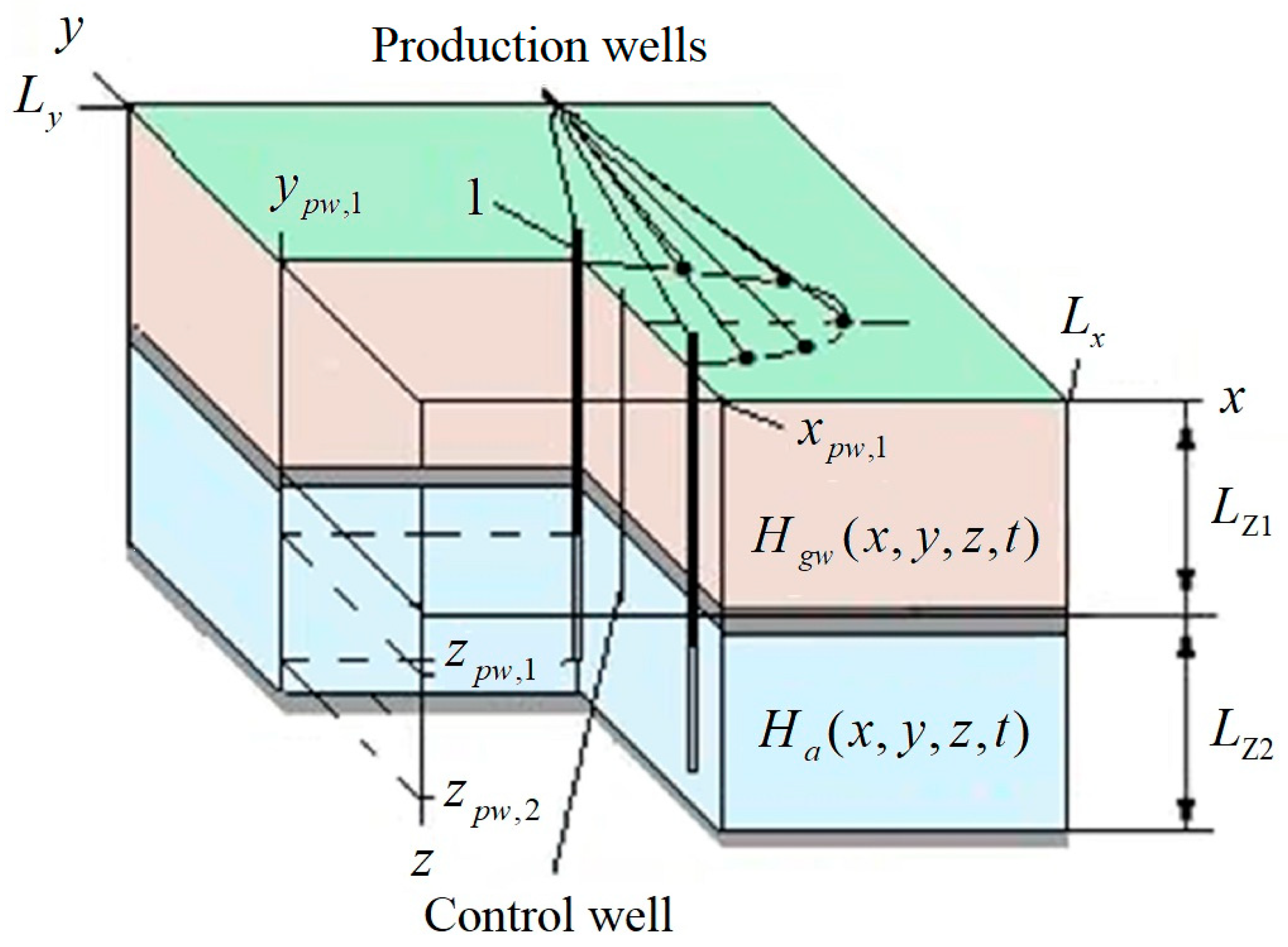
2. Materials and Methods

The development of the production MW wells network control system is based on the frequency analysis and synthesis concept for distributed systems. The theoretical provisions of this method are described in details in [1]. The mathematical model of the hydrogeological process for the MW deposit can be expressed as a partial differential transport equation [1,33]. The boundary conditions are selected based on the analysis of the structure of aquifers, according to the results of geological surveys [33,40,41]. The physical characteristics of aquifers can be set using the method of estimating parameters for aquifers based on experimental filtration operations under hydraulic connection conditions [1].

In this study, the dynamic characteristics of the control object were determined based on the results of experiments at production MW wells (Joint stock company “Narzan”, Kislovodsk, Russia). The hydrogeological profile of the Kislovodsk deposit is given in [1,39]. The estimation of variation in the dynamic characteristics of distributed objects during approximation is given in [1]. An approximating link was used to describe the static characteristics of the object under consideration [42]. The input effect on the object (pumping rate) is formed in the form of spatial modes [13].

The hydrogeologicalprocess for the MW deposit is considered as a control object, the scheme of which illustrated in Figure 1.

The cross section in Figure 1 shows free aquifer and confined aquifer separated by impervious layer. Production wells are located along the perimeter of the ellipse. The control well is used to monitor the pressure reduction in the confined aquifer.

Let us describe the groundwater flows in the free aquifer that lies on the first impervious layer from the surface by Equation (1) and in the confined aquifer by Equation (2) according to [1,33]:

$$\begin{array}{l}\frac{\partial H_{gw}(x,y,z,t)}{\partial t}=k_{gw,x}\times \frac{{\partial }^2{H}_{gw}(x,y,z,t)}{\partial x^2}+k_{gw,y}\times \frac{{\partial }^2{H}_{gw}(x,y,z,t)}{\partial y^2}+k_{gw,z}\times \frac{{\partial }^2{H}_{gw}(x,y,z,t)}{\partial z^2},\\ 0<x<L_x;\hspace{1em}0<y<L_y;\hspace{1em}0<z<L_{\mathrm{Z}1},\end{array}$$

(1)

$$\begin{array}{l}\frac{\partial H_a(x,y,z,t)}{\partial t}=\frac{1}{{\eta }_a}\times \left(k_{a,x}\times \frac{{\partial }^2{H}_a(x,y,z,t)}{\partial x^2}+k_{a,y}\times \frac{{\partial }^2{H}_a(x,y,z,t)}{\partial y^2}+k_{a,z}\times \frac{{\partial }^2{H}_a(x,y,z,t)}{\partial z^2}\right)+\\ +V(x_{pw,i},y_{pw,i},t)\times \delta (x_{pw,i},y_{pw,i},z_{pw,1}\le z\le z_{pw,2}),\\ V(x_{pw,i}, y_{pw,i}, t)=K_i\times Q_i(t),\hspace{1em}0<x<L_x;\hspace{1em}0<y<L_y;\hspace{1em}{L}_{\mathrm{Z}1}<z<L_{\mathrm{Z}2},\end{array}$$

(2)

where: H_gw is the water column height in the free aquifer, m; H_a is the water column height in the confined aquifer, m; k_gw,x, k_gw,y, k_gw,z are the hydraulic conductivities along spatial coordinates in the free aquifer, m/day, k_a,x, k_a,y, k_a,z are the hydraulic conductivities along spatial coordinates in the confined aquifer, m/day; x_pw,i, y_pw,i are coordinates of the location of production wells, m; η_a is the coefficient of elastic capacity, m⁻¹, in this case η_a = 1.6 × 10⁻³ m⁻¹; x, y, z are the spatial coordinates, m; N is number of wells, [–]; i is an order number of the production well, i = 1…N, [–]; t is time, day; a function δ(x_pw,i, y_pw,i, z_pw,1 ≤ z ≤ z_pw,2) = 1, if x = x_pw,i, y = y_pw,i, z_pw,1 ≤ z ≤ z_pw,2 (that corresponds to an imperfect water intake from an aquifer), and δ(x_pw,i, y_pw,i, z_pw,i ≤ z ≤ z_pw,i) = 0 in all other cases, [–]; V is a decrease in the water column height due to the impact of the production rate Q_i of the i-th well, m/day; K_i is a coefficient determined experimentally, in this case K_i = 0.187 m⁻²; Q_i(t) are production well rates, m³/day. In modeling, the condition was accepted that production rates are evenly distributed over the interval z_pw,1 ≤ z ≤ z_pw,2.

The hydraulic conductivities (m/day) along spatial coordinates are taken on the basis of experimental data: k_gw,x = 0.099; k_gw,y = 0.097; k_gw,z = 0.095; k_a,x = 0.199; k_a,y = 0.197; k_a,z = 0.108.

The leakage processes between free aquifer and the upper boundary of the confined aquifer are given in the following form:

$$\begin{gathered} \frac{\partial H_{gw}\left(x,y,L_{Z1},t\right)}{\partial t}=b_o\times \left(H_a\left(x,y,L_{Z1},t\right)-H_{gw}\left(x,y,L_{Z1},t\right)\right), \\ \frac{\partial H_a\left(x,y,L_{Z1},t\right)}{\partial t}=-b_o\times \left(H_a\left(x,y,L_{Z1},t\right)-H_{gw}\left(x,y,L_{Z1},t\right)\right), \end{gathered}$$

(3)

where b_o = 3 × 10⁻⁵ day⁻¹ is a leakage parameter.

For the lower boundary of the confined aquifer:

$$\frac{\partial H_a\left(x,y,L_{Z2},t\right)}{\partial z}=0.$$

(4)

For the lateral boundaries of the area under consideration:

$$\begin{array}{l}{H}_{gw}\left(0,y,z,t\right)=H_{gw}\left(L_x,y,z,t\right)=H_{gw}\left(x,0,z,t\right)=H_{gw}\left(x,L_y,z,t\right)=h_{gw,0},\\ H_a\left(0,y,z,t\right)=H_a\left(L_x,y,z,t\right)=H_a\left(x,0,z,t\right)=H_a\left(x,L_y,z,t\right)=H_{a,0}.\end{array}$$

(5)

When establishing boundary conditions along the y coordinate, it was assumed that the thickness of the confined aquifer is sufficient so that disturbances from production wells do not affect the state of the reservoir at the boundary points.

Initial conditions of undisturbed aquifers:

$$\begin{array}{l}{h}_{gw,0}\left(x,y,z,0\right)=z,\hspace{1em}0\le x\le L_x,\hspace{1em}0\le y\le L_y,\hspace{1em}0\le z\le L_{Z1},\\ H_{a,0}\left(x,y,z,0\right)=70-8\times x/L_{\mathrm{x}},\hspace{1em}0\le x\le L_x,\hspace{1em}0\le y\le L_y,\hspace{1em}{L}_{Z1}\le z\le L_{Z2}.\end{array}$$

(6)

Geometric data of the MW deposit: L_x = 150 m; L_y = 120 m; L_z1 = 55 m; L_z2 = 85 m.

Production wells are located along the perimeter of an ellipse, the half-axes of which are equal to a = 35 m, b = 20 m. The control well is offset along the y axis by a distance of 10 m relative to well 1.

3. Results

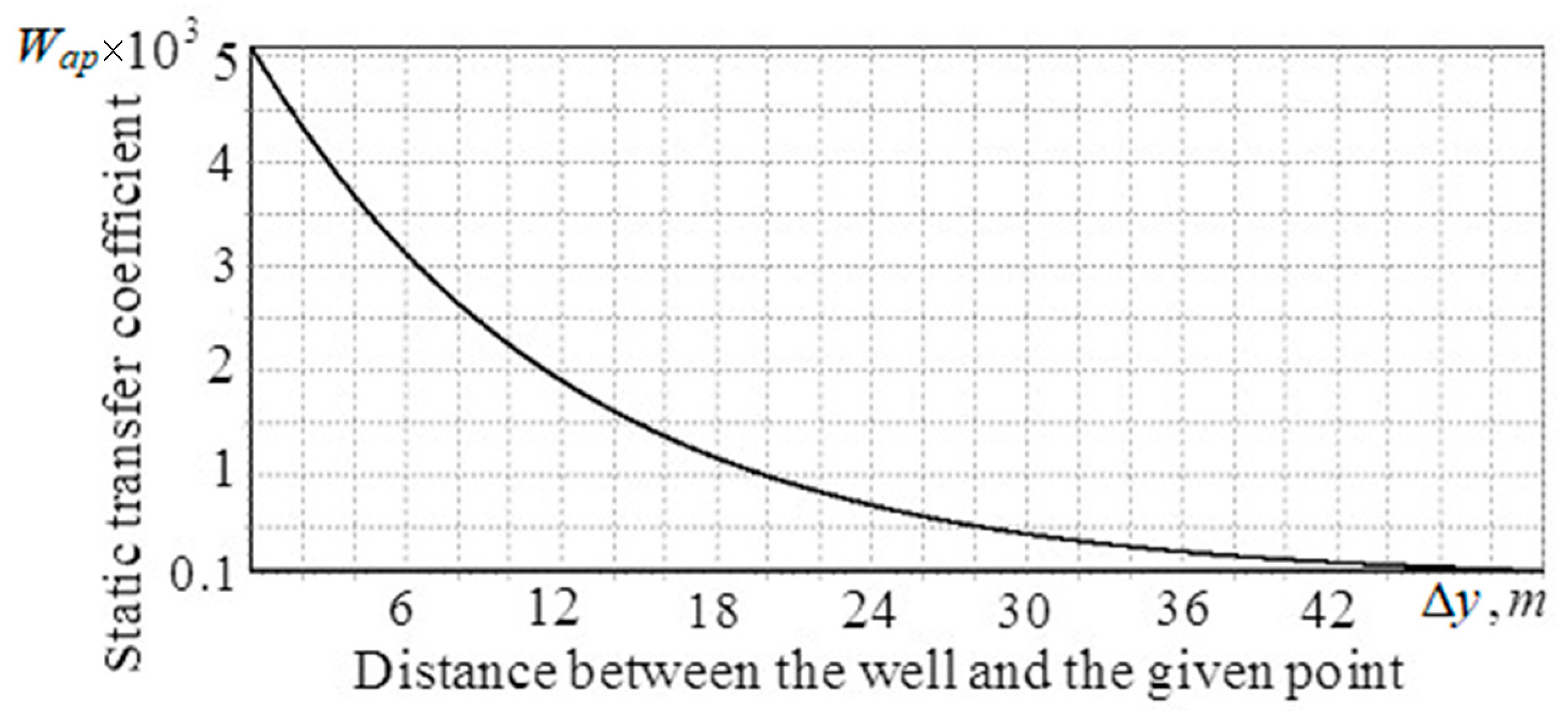
3.1. Study of the Characteristics of the Hydrogeological Process

Usually, during a mineral water field development, one production and one control wells are equipped. In this case, the production well 1 and the control well have equipment for measuring the level decrease. At the first stage, the operation of only these two wells was simulated in order to study the functional dependence between the level lowering in one well and the pumping rate of another well taking into account the distance between them.

In the course of experimental studies at the control object, a constant pumping rate in the production well was provided equal to Q₁ = 100 m³/day. This value was used to determine the static transfer coefficients K_p and K_c, respectively, for the production and control wells. The static transfer coefficient is equal to the steady-state level change in the corresponding well measured at the midpoint z = (z_pw,1 + z_pw,2)/2 m, divided by the pumping rate (input action) Q₁:

K_p = −0.512/(−100) = 5.12 × 10⁻³ m⁻²; K_c = −0.202/(−100) = 2.02 × 10⁻³ m⁻².

(7)

Structural schemes of approximating links for distributed objects have been considered in [33,42]. In these studies, it is shown that in the case of two wells, when describing the static characteristics of the object, the following structure of the approximating link can be recommended:

$$W_{ap}=\frac{K}{\sqrt{B}}\times \exp \left(-\sqrt{B}\times \Delta y\right),$$

(8)

where: W_ap is the transfer function of the approximating link; s is differential operator; K, B are parameters whose values are determined using experimental data or numerical modeling.

To find the parameters of the approximating link, the following data must be inserted into the Equation (8): static transfer coefficients K_p, K_c, as well as geometric data: the radius of the well Δy₁ = 0.2 m [1] and the distance between the production well 1 and the control well Δy₂ = 10 m.

$$\left\{\begin{array}{c}5.012\times {10}^{-3}=\frac{K}{\sqrt{B}}\times \exp \left(-\sqrt{B}\times 0.2\right),\\ 2.02\times {10}^{-3}=\frac{K}{\sqrt{B}}\times \exp \left(-\sqrt{B}\times 10\right).\end{array}\right.$$

(9)

The solution of the system of Equation (9) is that K = 4.9522 × 10⁻⁴ m⁻²; B = 9.007 × 10⁻³ [–].

Thus, the static transfer coefficient of an object can be written as Equation (10):

$$W_{ap}=\frac{4.9522\times {10}^{-4}}{\sqrt{9.007\times {10}^{-3}}}\cdot \exp \left(-\sqrt{9.007\times {10}^{-3}}\times \Delta y\right)=5.218\times {10}^{-3}\times \exp \left(-0.0949\times \Delta y\right),$$

(10)

where Δy is the distance from the well to the point under consideration, m.

Based on the simulation results, the plot of the static transfer coefficient of the object was presented as a function of the distance between the well and the given point (Figure 2).

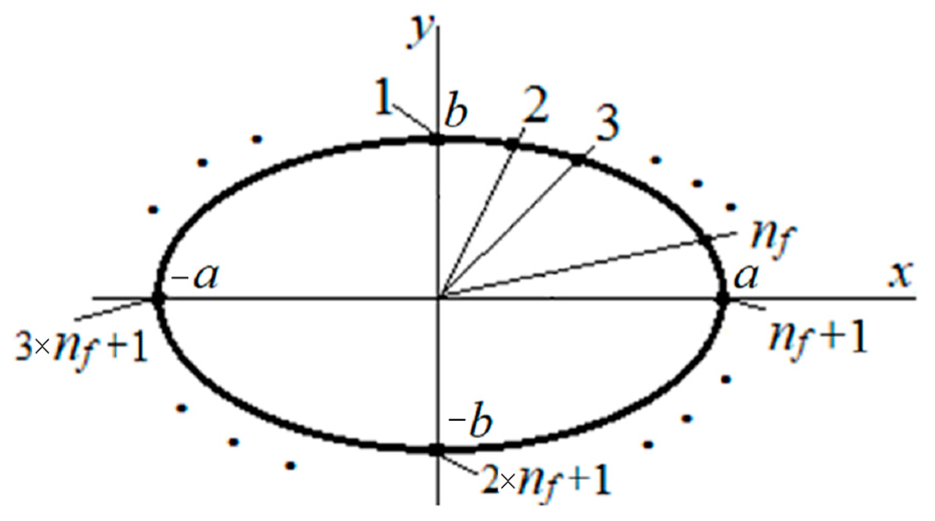
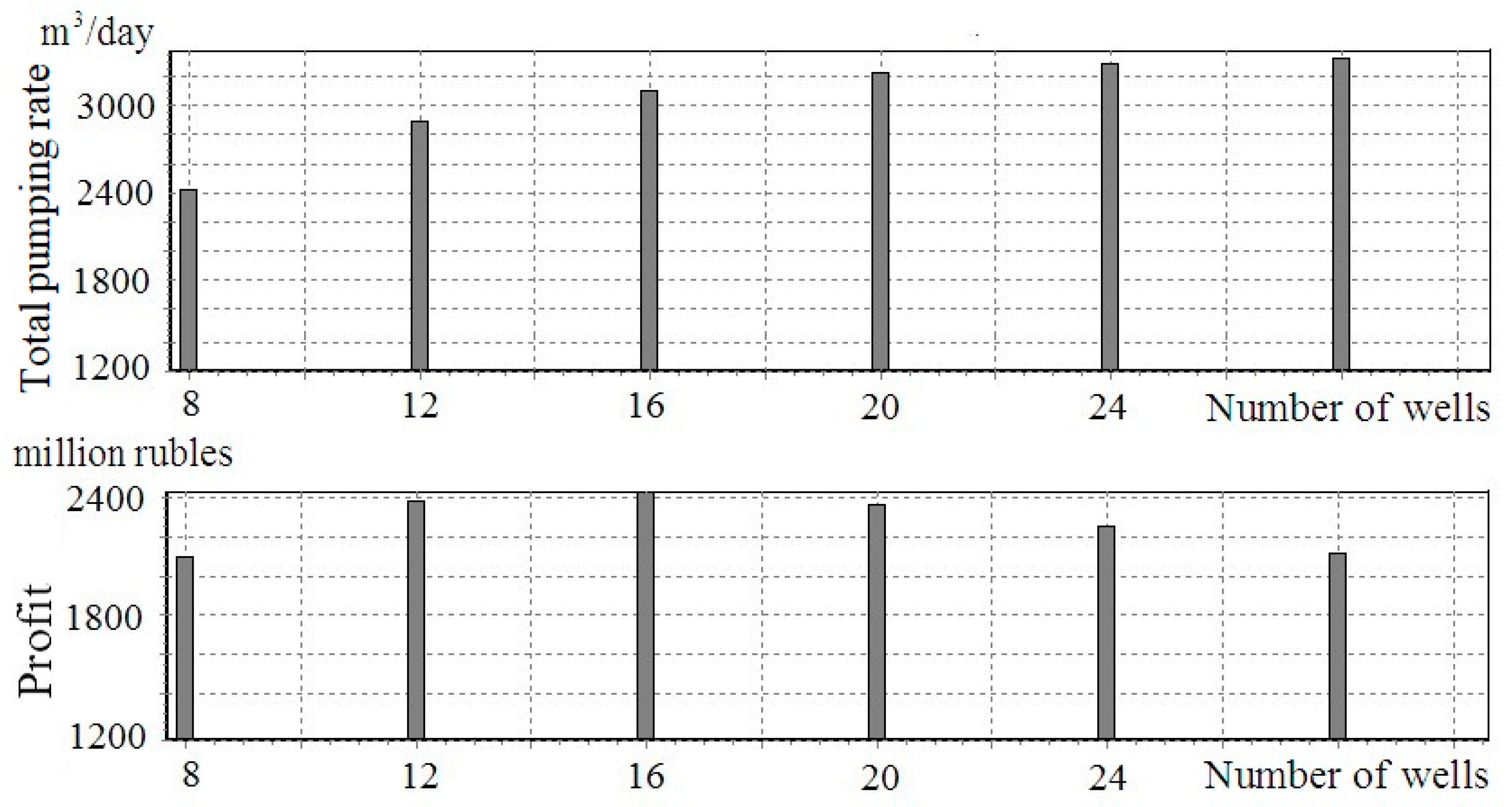
3.2. Determination of the Optimal Number of Production Wells

In the second stage of the control system development the simulation of the joint operation of the MW wells network in the form of an ellipse was performed. The layout is shown in Figure 3.

The coordinates of production wells are defined as follows: the first well is located at point 1 (x = x₁ = 0; y = y₁ = b); then the angle π/2 rad is divided into n_f parts. The canonical ellipse equation and the straight line equation are used to determine the coordinates of the second well:

$$\left\{\begin{array}{c}{y}_i=x_i\times tg\left(\frac{\pi }{2}\times \left(1-\frac{(i-1)}{n_f}\right)\right),\\ \frac{x_i{}^2}{a^2}+\frac{y_i{}^2}{b^2}=1.\end{array}\right.$$

(11)

The solution of the system of Equation (11) for the given values a, b, n_f and i provides the coordinates of the point i (x_i, y_i). The coordinates of the other points of the ellipse were defined in the similar way. A total of 4n_f points were obtained.

The problem of optimizing the number of production wells has the following statement: for the deposit under consideration (Figure 1 and Figure 3), it is necessary to determine the number of production wells (4n_f) that provide the highest profit for the period of operation of the deposit, taking into account the restrictions described below.

In this case, the following conditions must be met: the maximum permissible lowering of the level in the production wells ∆h = 2 m; well radius r_w = 0.2 m; MW wells operate 24 h per day for 10 years (3650 days); the cost of 1 m³ of extracted mineral water p₁ is 350 rubles; expenses for the maintenance of buildings and equipment and personnel for 10 years of operation C_p is 520 million rubles, the cost of drilling, construction, equipment and maintenance of each well for 10 years C is 45 million rubles; subsoil use tax is 7.5% [43].

The static transfer coefficient of the object is written by Equation (10). The effect of production wells pumping rate on lowering of the level in i-th production well in accordance with [42] can be represented as Equation (12):

$$\Delta h=\frac{K_i\times Q_i}{\sqrt{B}}\times \exp \left(-\beta \times \Delta r_w\right)+{\displaystyle \sum _{j=1,j\ne i}^{4nk}\frac{K_j\times Q_j}{\sqrt{B}}\times \exp \left(-\beta \times \Delta r_{i,j}\right)},\hspace{1em}i=1,\dots 4n_f,$$

(12)

where: ∆h is the lowering of the level in the i-th well (i = 1…4n_k), m; r_w is the radius of the well, m; ∆r_i,j is the distance from the i-th to the j-th interacting wells, m; Q_i, Q_j are the pumping rates of the i-th and j-th wells, m³/day.

In the mathematical model, Equation (7) was presented in matrix form. The total production rate Q can be determined as the sum of the n-well production rates:

$$Q={\displaystyle \sum _{i=1}^{4n_{\mathrm{f}}}{Q}_i.}$$

(13)

Knowing total production rate, the highest profit for 10 years of deposit operation can be estimated using Equation (14):

P = 3650 × Q × p₁ (1 − 0.075) − C_p − 4 × C × n_f.

(14)

Based on the results of calculations, the changes in the total pumping rate Q and profit P depending on the number of wells are shown in Figure 4.

As follows from the graphs, the maximum profit is achieved when using sixteen production wells. The projected income from the operation of the MW deposit for 10 years will amount to 2428.846 million rubles, at the total production rate of Q = 3104 m³/day.

3.3. Synthesis of a Distributed Controller

Method of synthesis of distributed controllers is reported in [1]. These scientific studies describe a number of dynamic distributed links by analogy with typical dynamic links. These links can be used to control objects with distributed parameters. Also in study [1] characteristics of dynamic distributed links are investigated, rationale for their choice and application is presented. Methods of modeling and transition from concentrated systems to systems with distributed parameters was shown in [44].

The development of the control system for the linear location of wells is described in [33]. In the case the production wells that are positioned in the shape of the ellipse, it is necessary to make the following modifications.

The spatial modes of the input action are formed as follows:

$$\begin{array}{l}{U}_i=Q\times \cos ({\psi }_{\mathrm{j}}\times {\gamma }_i ); \hspace{1em}{\psi }_j=2\times \pi \times j/L; \hspace{1em}\\ {\gamma }_i=\Delta \gamma \times (i-1);\hspace{1em}i=1, 2 , \dots 16;\hspace{1em}j=1, 2, \dots ,\end{array}$$

(15)

where: ψ_j is the spatial frequency; γ_i is the distance between two considered wells; Δγ is the distance between adjacent wells.

The spatial mode of the input action on the considered control object is distributed along the perimeter of the ellipse L, which is equal to 176.5 m. The formation of the first mode (j = 1) of the input action is shown in Figure 5. Other spatial modes are formed in a similar way (j = 2, 3, …).

As a rule, in accordance with the method of synthesis of distributed control systems, it is necessary to determine the reaction of an object to any two spatial modes. The first mode is formed in the space {γ}, and is implemented at the given points (x_pw,i, y_pw,i) in the space {x, y} (at the points of location of the production wells). If the calculated value U_i (i = 1… 16) is displayed in the space {x, y}, then the following expression can be obtained:

$$U(x_{pw,i},y_{pw,i})=U_i,\hspace{1em}V(x_{pw,i},y_{pw,i},t)=K_i\times U(x_{pw,i},y_{pw,i}),\hspace{1em}i=1\dots 16.$$

(16)

Mathematical modeling allows determining the response of the object to the first and second spatial modes (Equation (15)), and calculating the transfer coefficient of the control object for the considered modes of the input action. The calculated values of the transfer coefficients (K₁ and K₂) and the generalized coordinate (G₁ and G₂) were determined as:

K₁ = 775.0 m⁻²; G₁ = ψ₁² = (2 × π × 1/L)² = 1.003 × 10⁻³ [–]; K₂ = 583.3 m⁻²; G₂ = ψ₂² = (2 × π × 2/L)² = 4.01 × 10⁻³ [–].

(17)

Based on the modeling, the plots of the input action and the output function were drawn for all wells, which allowed determining the phase shift of the output function relative to the input action. The graphs of the input action and the output function for the production well 8 is shown in Figure 6.

Further, the phase shift of the output function relative to the input action is determined graphically:

∆φ = 2 × π × (−2.214)/17.45 = −0.797 rad.

(18)

It is shown in [33,39] that the dynamic characteristics of objects with a linear location of the well network can be described by the following structure of approximating links:

$$W_{ap}(s,G)=\frac{K}{\beta +1}\times \exp \left(-\beta \times D_{\gamma }\right), \hspace{1em}\beta ={\left(\frac{s}{a}+G\right)}^{0.5},\hspace{1em}{G}_j\le G\le \infty ,$$

(19)

where: K, a, D_γ are the defined parameters.

Using the previously calculated values K₁ = 775.0 m⁻²; G₁ = 1.003 × 10⁻³ [–]; K₂ = 583.3 m⁻²; G₂ = 4.01 × 10⁻³ [–]; ∆φ = −0.797 rad, an approximation model of the control object was determined:

$$W_{ap}(s,G)=\frac{1030.67}{1+\sqrt{\frac{s}{5.916\times {10}^{-3}}+G}}\times \exp \left(-8.02\times \sqrt{\frac{s}{5.916\times {10}^{-3}}+G}\right),\hspace{1em}{G}_1\le G\le \infty .$$

(20)

The transfer function of the distributed controller [1,13] can be written as:

$$W\left(\gamma ,s\right)=E_a\times \left(\frac{n_a-1}{n_a}-\frac{1}{n_a}{\nabla }^2\right)+E_i\times \left(\frac{n_i-1}{n_i}-\frac{1}{n_i}{\nabla }^2\right)\times \frac{1}{s}+E_d\times \left(\frac{n_d-1}{n_d}-\frac{1}{n_d}{\nabla }^2\right)\times s,$$

(21)

where: E_a, E_i, E_d are the overall gains of the spatially amplifying, spatially integrating and spatially differentiating links, respectively; γ is the spatial coordinate; s is differential operator; ${\nabla }^2$ is Laplacian; n_a, n_i, n_d are weighting factors of the spatially amplifying, spatially integrating, and spatially differentiating links.

During the synthesis of the distributed controller, the following restrictions must be taken into account: phase stability margin ∆φ ≥ π/6 rad; stability margin modulo ∆L ≥ 10 dB; parameter that takes into account parametric disturbances of the control object ∆ = 2.5 [–].

As a result of the implementation of the synthesis procedure, parameters of distributed controller (Equation (21)) are obtained: E_a = 0.22999 m², E_i = 0.00108 m², E_d = 7.71 m²_, n_a = 1.065 [–], n_i = 1.0859 [–], n_d $\to$ ∞ [–].

4. Discussion

Thus, when forming the control action for each of the well location points, the mismatch and the accumulated error both at the given and neighboring points will be taken into account, while the differential link will form the corresponding component of the control action only based on the change rate of the mismatch at a given point.

The block diagram of a distributed control system for a MW well network positioned in the form of an ellipse is shown in Figure 7.

To analyze the operation of a closed loop control system, a signal ∆H_a(i,t) is sent to the input of the controller, this signal is a mismatch between the desired value of the level H_ad(i,t) in the well location zones and the current value of the level H_a(i,t):

∆H_a (i,t) = H_ad (i,t) − H_a(i,t),  i = 1, 2, …, 16.

(22)

The output is the function Q_i (pumping rate of the i-th production well):

$$\begin{array}{c}{Q}_i(t)=0.22999\times \left(\frac{0.065}{1.065}\times \Delta H_a(i,t)-\frac{1}{1.065}\times {\nabla }^2\Delta H_a(i,t)\right)+\\ +0.00108\times {\displaystyle \underset{0}{\overset{t}{\int }}\left(\frac{0.0859}{1.0859 }\times \Delta H_a(i,\tau )-\frac{1}{1.0859}\times {\nabla }^2\Delta H_a(i,\tau )\right)}d\tau +7.71\times \frac{d\Delta H_a(i,t)}{dt},\\ i=1,\dots 16,\end{array}$$

(23)

$$\begin{gathered} {\nabla }^2\Delta H_a(i,t)=\frac{\Delta H_a(i-1,t)-2\times \Delta H_a(i,t)+\Delta H_a(i+1,t)}{\Delta {\gamma }^2}, i=2,\dots 15, \\ {\nabla }^2\Delta H_a(1,t)=\frac{\Delta H_a(16,t)-2\times \Delta H_a(1,t)+\Delta H_a(2,t)}{\Delta {\gamma }^2}, \\ {\nabla }^2\Delta H_a(16,t)=\frac{\Delta H_a(15,t)-2\times \Delta H_a(16,t)+\Delta H_a(1,t)}{\Delta {\gamma }^2}. \end{gathered}$$

(24)

Based on the results of modeling the operation of a closed loop control system, transient graphs were obtained for all wells, which allowed us to assess the quality of regulation. Transient graph for the MW well 13 is shown in Figure 8.

According to the graph, it can be seen that the level of stabilization (zero misalignment) can be achieved after 13.25 h when the input action is applied and conclude that the obtained parameters of the controller can ensure stable operation of the control system under the specified restrictions.

Thus, a model of a distributed control system for a network of mineral water production wells has been developed. The novelty of the proposed model lies in the fact that, in comparison with previous models with a linear configuration of the MW network, the elliptical shape of the location of the MW wells was investigated. The elliptical configuration more accurately reflects the natural boundaries of the explored mineral and artesian water deposits [1]. Due to the consideration of another area of the MV field, a quantitative comparison of this model with the model presented in the study [33] is not possible. However, the linear configuration of wells during field development is not always possible due to the peculiarities of the terrain of the region under consideration and the need to preserve natural monuments, as well as objects of historical and cultural heritage. In addition, the elliptical location of production wells will allow equipping the MW field based on the conditions of proximity of mineralization levels and piezometric levels in the wells of the field if the isolines of these levels are close to elliptical, which is common for the region under consideration [1].

For the first time, the article presents an algorithm for developing a distributed control system for the considered well network, as well as solving practical problems, including determining dynamic characteristics for the control object under study and calculating the parameters of a distributed controller. Based on the results of modeling the operation of a closed loop control system, a transition processes schedules were obtained, which makes it possible to evaluate the quality indicators of the control process. When studying the hydrogeological processes, it is necessary to consider the influence of random factors. The issues of control of hydrodynamic processes under random impacts in the aquifers of mineral water deposits considered in [45]. The influence of random factors can be largely leveled by introducing feedback into the system, which is implemented in this work.

The advantages of a feedback system are regulation by deviation from the set value and robustness. Regulation by deviation from the set value (i.e., based on the results of current measurements) allows us to take into account changes in productivity during the operation of the field. Robustness (low sensitivity to parametric disturbances) makes it possible to maintain a given value of the output function (level lowering in production wells) with some changes in the parameters of the object, for example, hydraulic conductivity. The degree of robustness of the synthesized system can be the object of further research.

Also, the optimal number of production wells was found, based on the condition of maximum economical profit for the specified period of the deposit operation (for 10 years). When solving the problem, the restriction in the form of acceptable lowering of of the level in the production wells is taken into account. The projected income from the operation of the deposit for 10 years is approximately 2428.846 ruble for the total production rate of MW of Q = 3104 m³/day.

The development is based on the frequency analysis and synthesis concept for distributed control systems. An important advantage of the frequency controller synthesis method is the possibility of developing mathematical models based on the dynamic characteristics of the object obtained experimentally.

5. Conclusions

The article presents a solution to the theoretical problem of developing an algorithm for the synthesis of a distributed control system with the location of production wells in the form of an ellipse. The practical problems were also solved. The optimal number and pumping rate of production wells in the well network providing the maximum profit for the enterprise during a given operation period of the deposit have been determined. The dynamic characteristics for the control object under consideration, as well as the parameters of a distributed controller for the control system of the network of mineral water wells have been calculated.

The developed algorithm for the synthesis of a distributed control system for a deposit, in which the production wells are located in an ellipse, can be applied to both free and confined aquifers with different thickness, length, lithology, hydraulic conductivity by making appropriate changes to the original mathematical model. The description of the boundary conditions can also be changed when considering another (or larger) area of the deposit, which may be a direction for further research, but does not entail restrictions in the application of the proposed algorithm for the synthesis of a mineral water well network control system.

The effectiveness of the proposed approach is confirmed by the results of modeling. The proposed model can be used for operational monitoring and forecasting of hydrogeological processes and creating a regional management system for mineral water production in the network of explored deposits.

References

1. Malkov, A.V.; Pershin, I.M.; Pomelyayko, I.S.; Utkin, V.A.; Korolev, B.I.; Dubogrey, V.F.; Khmel, V.V.; Pershin, M.I. Kislovodsk Carbon Dioxide Mineral Water Field: System Analysis, Diagnostics, Forecast, Control; Nauka: Moscow, Russia, 2015; ISBN 978-5-02-039162-8. (In Russian) [Google Scholar]
2. Pomelyaiko, I.S.; Malkov, A.V. Quality Problems of Surface Water and Groundwater at the Health Resorts in the Regions of Caucasian Mineral Waters and Ways to Their Solution. Water Resour. 2019, 46, 214–225. [Google Scholar] [CrossRef]
3. Drovosekova, T.I.; Rusak, S.N.; Harish, N.P. Issues of and outlook for using geothermal water. In Proceedings of the 2019 International Science and Technology Conference “EastConf”, Vladivostok, Russia, 1–2 March 2019; p. 8725307. [Google Scholar] [CrossRef]
4. Karlović, I.; Marković, T.; Smith, A.C.; Maldini, K. Impact of Gravel Pits on Water Quality in Alluvial Aquifers. Hydrology 2023, 10, 99. [Google Scholar] [CrossRef]
5. Semyachkov, A.I.; Pochechun, V.A.; Semyachkov, K.A. Hydrogeoecological conditions of technogenic groundwater in waste disposal sites. J. Min. Inst. 2023, 260, 168–179. [Google Scholar] [CrossRef]
6. Wang, J.; Xu, J. Spatial Distribution and Controlling Factors of Groundwater Quality Parameters in Yancheng Area on the Lower Reaches of the Huaihe River, Central East China. Sustainability 2023, 15, 6882. [Google Scholar] [CrossRef]
7. Ostad, H.; Mohammadi, Z.; Fiorillo, F. Assessing the Effect of Conduit Pattern and Type of Recharge on the Karst Spring Hydrograph: A Synthetic Modeling Approach. Water 2023, 15, 1594. [Google Scholar] [CrossRef]
8. Ahamed, A.; Knight, R.; Alam, S.; Morphew, M.; Susskind, T. Remote Sensing-Based Estimates of Changes in Stored Groundwater at Local Scales: Case Study for Two Groundwater Subbasins in California’s Central Valley. Remote Sens. 2023, 15, 2100. [Google Scholar] [CrossRef]
9. Ramos, E.; Bux, R.K.; Medina, D.I.; Barrios-Piña, H.; Mahlknecht, J. Spatial and Multivariate Statistical Analyses of Human Health Risk Associated with the Consumption of Heavy Metals in Groundwater of Monterrey Metropolitan Area, Mexico. Water 2023, 15, 1243. [Google Scholar] [CrossRef]
10. Gad, M.; Gaagai, A.; Eid, M.H.; Szűcs, P.; Hussein, H.; Elsherbiny, O.; Elsayed, S.; Khalifa, M.M.; Moghanm, F.S.; Moustapha, M.E.; et al. Groundwater Quality and Health Risk Assessment Using Indexing Approaches, Multivariate Statistical Analysis, Artificial Neural Networks, and GIS Techniques in El Kharga Oasis, Egypt. Water 2023, 15, 1216. [Google Scholar] [CrossRef]
11. Golovina, E.; Shchelkonogova, O. Possibilities of Using the Unitization Model in the Development of Transboundary Groundwater Deposits. Water 2023, 15, 298. [Google Scholar] [CrossRef]
12. Golovina, E.; Pasternak, S.; Tsiglianu, P.; Tselischev, N. Sustainable Management of Transboundary Groundwater Resources: Past and Future. Sustainability 2021, 13, 12102. [Google Scholar] [CrossRef]
13. Shestopalov, M.Y.; Pershin, I.M.; Tsapleva, V.V. Distributed Control Systems Designing. In Proceedings of the 2019 III International Conference on Control in Technical Systems (CTS), St. Petersburg, Russia, 30 October–1 November 2019; pp. 85–88. [Google Scholar] [CrossRef]
14. Pershin, I.M.; Papush, E.G.; Malkov, A.V.; Kukharova, T.V.; Spivak, A.O. Operational Control of Underground Water Exploitation Regimes. In Proceedings of the 2019 III International Conference on Control in Technical Systems (CTS), St. Petersburg, Russia, 30 October–1 November 2019; pp. 77–80. [Google Scholar] [CrossRef]
15. Grigorev, G.S.; Salishchev, M.V.; Senchina, N.P. On the applicability of electromagnetic monitoring of hydraulic fracturing. J. Min. Inst. 2021, 250, 492–500. [Google Scholar] [CrossRef]
16. Zhukovskiy, Y.L.; Korolev, N.A.; Malkova, Y.M. Monitoring of grinding condition in drum mills based on resulting shaft torque. J. Min. Inst. 2022, 256, 686–700. [Google Scholar] [CrossRef]
17. Martirosyan, A.V.; Ilyushin, Y.V. The Development of the Toxic and Flammable Gases Concentration Monitoring System for Coalmines. Energies 2022, 15, 8917. [Google Scholar] [CrossRef]
18. Zakharov, L.A.; Martyushev, D.A.; Ponomareva, I.N. Predicting dynamic formation pressure using artificial intelligence methods. J. Min. Inst. 2022, 253, 23–32. [Google Scholar] [CrossRef]
19. Arefiev, I.B.; Afanaseva, O.V. Implementation of Control and Forecasting Problems of Human-Machine Complexes on the Basis of Logic-Reflexive Modeling. Lect. Notes Netw. Syst. 2022, 442, 187–197. [Google Scholar] [CrossRef]
20. Kovalev, D.A.; Rusinov, L. Increase in environmental safety of recovery boiler. IOP Conf. Ser. Earth Environ. Sci. 2022, 990, 012068. [Google Scholar] [CrossRef]
21. Veselov, G.E.; Sinicyn, A. Synthesis of sliding control system for automotive suspension under kinematic constraints. J. Vibroengineering 2021, 23, 1446–1455. [Google Scholar] [CrossRef]
22. Pershin, I.M.; Liashenko, A.L.; Papush, E.G. General Principles for Designing Distributed Control Systems. In Proceedings of the 2020 Wave Electronics and its Application in Information and Telecommunication Systems (WECONF), St. Petersburg, Russia, 1–5 June 2020; pp. 1–6. [Google Scholar] [CrossRef]
23. Makarova, A.A.; Kaliberda, I.V.; Kovalev, D.A.; Pershin, I.M. Modeling a Production Well Flow Control System Using the Example of the Verkhneberezovskaya Area. In Proceedings of the 2022 Conference of Russian Young Researchers in Electrical and Electronic Engineering, St. Petersburg, Russia, 25–28 January 2022; pp. 760–764. [Google Scholar] [CrossRef]
24. Sizov, S.; Drovosekova, T.; Pershin, I. Application of Machine Learning Methods in Modeling Hydrolithospheric Processes. Commun. Comput. Inf. Sci. 2021, 1395, 422–431. [Google Scholar] [CrossRef]
25. Tsapleva, V.V.; Masyutina, G.V.; Danchenko, I.V. Construction of a mathematical model for the extraction of mineral raw materials. IOP Conf. Ser. Earth Environ. Sci. 2020, 613, 012154. [Google Scholar] [CrossRef]
26. Pershin, I.; Sidyakin, P.; Belaya, E.; Shchitov, D. Modeling the formation of acoustic resonant waves in a closed space. IOP Conf. Ser. Mater. Sci. Eng. 2019, 698, 077054. [Google Scholar] [CrossRef]
27. Martirosyan, A.V.; Martirosyan, K.V.; Mir-Amal, A.M.; Chernyshev, A.B. Assessment of a Hydrogeological Object’s Distributed Control System Stability. In Proceedings of the 2022 Conference of Russian Young Researchers in Electrical and Electronic Engineering, St. Petersburg, Russia, 25–28 January 2022; pp. 768–771. [Google Scholar] [CrossRef]
28. Grigoriev, V.V.; Bystrov, S.V.; Mansurova, O.K.; Pershin, I.M.; Bushuev, A.B.; Petrov, V.A. Exponential stability regions estimation of nonlinear dynamical systems. Mekhatronika Avtom. Upr. 2020, 21, 131–135. [Google Scholar] [CrossRef]
29. Dagaev, A.; Pham, V.D.; Kirichek, R.; Afanaseva, O.; Yakovleva, E. Method of Analyzing the Availability Factor in a Mesh Network. Commun. Comput. Inf. Sci. 2022, 1552, 346–358. [Google Scholar] [CrossRef]
30. Liashenko, A.L.; Pershin, I.M.; Moreva, S.L. Development of a Distributed System of Control of the Supply of the Coolant in Steam Generator Installations. In Proceedings of the 2020 Wave Electronics and its Application in Information and Telecommunication Systems (WECONF), St. Petersburg, Russia, 1–5 June 2020; pp. 1–5. [Google Scholar] [CrossRef]
31. Fetisov, V.; Ilyushin, Y.V.; Vasiliev, G.G.; Leonovich, I.A.; Müller, J.; Riazi, M.; Mohammadi, A.H. Development of the automated temperature control system of the main gas pipeline. Sci. Rep. 2023, 13, 3092. [Google Scholar] [CrossRef] [PubMed]
32. Martirosyan, A.V.; Ilyushin, Y.V.; Afanaseva, O.V. Development of a Distributed Mathematical Model and Control System for Reducing Pollution Risk in Mineral Water Aquifer Systems. Water 2022, 14, 151. [Google Scholar] [CrossRef]
33. Pershin, I.M.; Malkov, A.V.; Pomelyayko, I.S. Design of a Distributed Debit Management Network of Operating Wells of Deposits of the CMW Region. Commun. Comput. Inf. Sci. 2021, 1396, 317–328. [Google Scholar] [CrossRef]
34. Satsuk, T.P.; Sharyakov, V.A.; Sharyakova, O.L.; Kovalev, D.A.; Vorob’ev, A.A.; Makarova, E.I. Erratum to: Automatic Voltage Stabilization of an Electric Rolling Stock Catenary System. Russ. Electr. Eng. 2021, 92, 349. [Google Scholar] [CrossRef]
35. Tsiglianu, P.; Romasheva, N.; Nenko, A. Conceptual Management Framework for Oil and Gas Engineering Project Implementation. Resources 2023, 12, 64. [Google Scholar] [CrossRef]
36. González de Vallejo, L.I.; Ferrer, M.; Ortuño, L.; Oteo, C. Ingeniería Geológica; Prentice Hall-Pearson Educación: Madrid, Spain, 2002; p. 750. [Google Scholar]
37. Ayvaz, M.T.; Karahan, H. A Simulation/Optimization Model for the Identification of Unknown Groundwater Well Locations and Pumping Rates. J. Hydrol. 2008, 357, 76–92. [Google Scholar] [CrossRef]
38. Ilyushin, Y.V.; Afanaseva, O.V. Development of scada-model for trunk gas pipeline’s compressor station. J. Min. Inst. 2019, 240, 686–693. [Google Scholar] [CrossRef] [Green Version]
39. Ilyushin, Y.V.; Asadulagi, M.-A.M. Development of a Distributed Control System for the Hydrodynamic Processes of Aquifers, Taking into Account Stochastic Disturbing Factors. Water 2023, 15, 770. [Google Scholar] [CrossRef]
40. Li, Y.; Zhou, Z.; Zhuang, C.; Dou, Z. Estimating Hydraulic Parameters of Aquifers Using Type Curve Analysis of Pumping Tests with Piecewise-Constant Rates. Water 2023, 15, 1661. [Google Scholar] [CrossRef]
41. Angelaki, A.; Bota, V.; Chalkidis, I. Estimation of Hydraulic Parameters from the Soil Water Characteristic Curve. Sustainability 2023, 15, 6714. [Google Scholar] [CrossRef]
42. Pershin, M.I.; Papush, E.G.; Spivak, A.O. Approximation Models for the Hydrolitospheric Processes. In Proceedings of the 2018 International Multi-Conference on Industrial Engineering and Modern Technologies (FarEastCon 2018), Vladivostok, Russia, 2–4 October 2018; pp. 1–6. [Google Scholar] [CrossRef]
43. Nosova, V.A.; Pershin, I.M. Determining the optimal number of wells during field development. In Proceedings of the 2021 4th International Conference on Control in Technical Systems (CTS 2021), St. Petersburg, Russia, 21–23 September 2021; pp. 42–44. [Google Scholar] [CrossRef]
44. Ilyushin, Y.V.; Afanasieva, O.V. Synthesis of a distributed control system. Int. J. Control Theory Appl. 2016, 9, 41–60. [Google Scholar]
45. Asadulagi, M.M.; Ioskov, G.V. Simulation of the control system for hydrodynamic process with random disturbances. Topical Issues of Rational Use of Natural Resources. In Proceedings of the International Forum-Contest of Young Researchers, St. Petersburg, Russia, 18–20 April 2018; pp. 399–405. [Google Scholar]
Figure 1. Mineral water (MW) deposit scheme with control and production wells.
Water 15 02289 g001
Figure 2. Static transfer coefficient Wapy) as a function of distance.
Water 15 02289 g002
Figure 3. Layout of wells.
Water 15 02289 g003
Figure 4. Changes in the total pumping rate Q and profit P depending on the number of wells.
Water 15 02289 g004
Figure 5. Formation of the first spatial mode.
Water 15 02289 g005
Figure 6. Graphs of input action and output function.
Water 15 02289 g006
Figure 7. Block diagram of a distributed control system for a MW well network.
Water 15 02289 g007
Figure 8. Transient graph for well 13.
Water 15 02289 g008
Disclaimer/Publisher’s Note: The statements, opinions and data contained in all publications are solely those of the individual author(s) and contributor(s) and not of MDPI and/or the editor(s). MDPI and/or the editor(s) disclaim responsibility for any injury to people or property resulting from any ideas, methods, instructions or products referred to in the content.