Meteorological and Hydrological Drought Risk Assessment Using Multi-Dimensional Copulas in the Wadi Ouahrane Basin in Algeria

Abstract

A persistent precipitation deficiency (meteorological drought) could spread to surface water bodies and produce a hydrological drought. Meteorological and hydrological droughts are thus closely related, even though they are separated by a time lag. For this reason, it is paramount for water resource planning and for drought risk analysis to study the connection between these two types of drought. With this aim, in this study, both meteorological and hydrological drought were analyzed in the Wadi Ouahrane Basin (Northwest Algeria). In particular, data from six rainfall stations and one hydrometric station for the period 1972–2018 were used to evaluate the Standardized Precipitation Index (SPI) and the Standardized Runoff Index (SRI) at multiple timescales (1, 2, 3, 4, …, 12 months). By means of a copula function, the conditional return period for both types of drought was evaluated. Results evidenced that runoff is characterized by high level of temporal correlation in comparison to rainfall. Moreover, the composite index JDHMI (Joint Deficit Hydro-meteorological Index) was evaluated. This index is able to reflect the simultaneous hydrological and meteorological behavior at different timescales of 1–12 months well and can present the probability of a common hydrological and meteorological deficit situation more accurately and realistically compared to precipitation or runoff-based indicators. It was found that, over the analyzed basin, the average severity of combined hydro-meteorological drought (JDHMI) was 10.19, with a duration of 9 months and a magnitude of 0.93.

1. Introduction

In recent years, modifications in catchment dynamics as a consequence of environmental and climate changes have been observed. In fact, both human impact and climate variability can affect the hydrological processes of a river catchment [1,2], with consequences for water resources, hydropower production [3,4], and crop yield [5]. Indeed, depending on the region, the climate variability can increase or decrease the components of the hydrological regime. As an example, in Morocco, the authors of [6] analyzed future streamflow regimes by means of the Indicator of Hydrological Alterations (IHA) and detected that, under future changes in climate patterns, flow regimes, expressed as monthly flow magnitude and frequency flow pulses, can be altered. Such changes would in turn influence the ecological status of a river. Ref. [7], by analysing future climate prediction for the Heihe River basin in northwest China, concluded that climate change may affect stream ecosystems through flow regime alterations. Henriksen et al. [8] showed significant changes in the freshwater cycle with climate factors in two large-scale catchments in Denmark. At the same time, at higher elevations or latitudes, climate change is expected to weaken the modulating effect of snow and glacier fields, with possibly strong impacts on hydropower generation, floods and droughts, irrigation water supplies, and associated food production [9]. Moreover, the variability of a hydrological regime is strongly affected by anthropogenic actions such as irrigation, urbanization, and recreational activities [10]. In particular, land cover change is a dominant factor affecting ecosystems [11,12] and the hydrological regime [13]. For example, Lopez et al. [14] detected that forest conversion to agriculture use has directly affected the surface runoff and groundwater contribution of the Upper Teles Pires (Brazil). Zhang et al. [15] evidenced that the watershed size influences the sensitivity of annual runoff to forest cover change and that annual runoff is more sensitive to forest cover change in water-limited watersheds than in energy-limited watersheds. In a study proposed by Dorjsuren et al. [16] in Mongolia, it was pointed out that land cover changes are directly linked to the hydro-meteorological parameters and that in arid and semi-arid regions, climate change significantly impacts land cover changes. Wojkowski et al. [17] examined landscape hydric potential as a descriptor of water storage and showed that land cover can influence the predictability of maximum annual flow in a mountainous region of central Europe.

Drought, which is characterized by a high spatial and temporal variability [18], is currently one of the main global problems for water resources and has significant environmental, social, and economic consequences [19]. In particular, the investigation of the relation between meteorological and hydrological drought is important for water management and early warning and mitigation at the basin scale [20]. In fact, meteorological and hydrological droughts are inherently correlated, but with a time lag [21]. Knowledge of this relationship can be used for water resource planning and for developing drought resistance measures. This relationship can be represented, e.g., by copula-based bivariate probabilities [22]. Ding et al. [23], by analyzing meteorological and hydrological drought in China, highlighted a weaker propagation relationship in arid environments than in moist environments and evidenced a stronger relationship between the two types of drought, especially in summer and autumn. Bevacqua et al. [24] indicated that, over 457 basins in Brazil, hydrological droughts are usually more long-lasting, severe, and with a slower recovery time compared to meteorological droughts. Moreover, hydrometeorological variables very often are non-stationary, so there is justification for introducing time dependence into the definition of standardized drought indices. In this context, Zhang et al. [25] introduced the Nonstationary Meteorological and Hydrological Drought Index (NMHDI) and detected that the time-varying copula model can better predict the drought induced under a changing environment in the Weihe River Basin (western China). Ho et al. [26] applied run theory to a high-resolution remote sensing daily dataset to analyze some standardized drought indices representing precipitation, runoff, evapotranspiration, and soil moisture in the Central Asian subcontinent. As shown by Zhu et al. [20], a traditional statistical model can be inappropriate in drought analyses, while a copula-based conditional distribution method can provide a satisfactory probabilistic prediction of hydrological drought characteristics based on the information about meteorological drought characteristics. Gu et al. [27], using copulas, analyzed drought in three catchments of China and detected that drought shows lengthened duration, amplified severity, and time-delay phenomena among these catchments. In order to analyze drought characteristics and the connection between meteorological and hydrological droughts over the Yellow River basin, Zhu et al. [20] proposed a probabilistic framework based on the copula function. Farrokhi et al. [28] introduced a new methodology for modeling multivariate dependence structures of meteorological drought characteristics based on the combination of four-dimensional vine copulas and a data mining algorithm. Wang et al. [29] used the Frank copula to analyze meteorological and hydrological drought in the Yellow River basin.

With regard to Algeria, several studies, e.g., [30,31,32], have been performed on meteorological drought using the Standardized Precipitation Index (SPI). However, although in an arid and semi-arid country such as Algeria the problem of water scarcity caused by the strong spatial and temporal variability of precipitation is pervasive, a coupled analysis of meteorological and hydrological drought has not been performed [33]. The application of the composite index JDHMI, to analyze meteorological and hydrological drought in this region, better reflects actual problems with water resources. In fact, this index includes the main sources of drought, i.e., the deficit of precipitation that in consequence results in decreasing flow. Moreover, a more complex index of drought can be an excellent tool for decision makers to analyze drought and water management in regards to mitigation activities to prevent drought. In this context, the objective of this study is thus to investigate both meteorological and hydrological drought in the Wadi Ouahrane Basin (northwest Algeria) by using two standard drought indices, the SPI for meteorological drought and the SRI for hydrological drought, evaluated at different timescales (1, 2, 3, 4, …, 12 months). In particular, the conditional return period for both types of drought will be evaluated by means of copula functions.

2. Materials and Methods

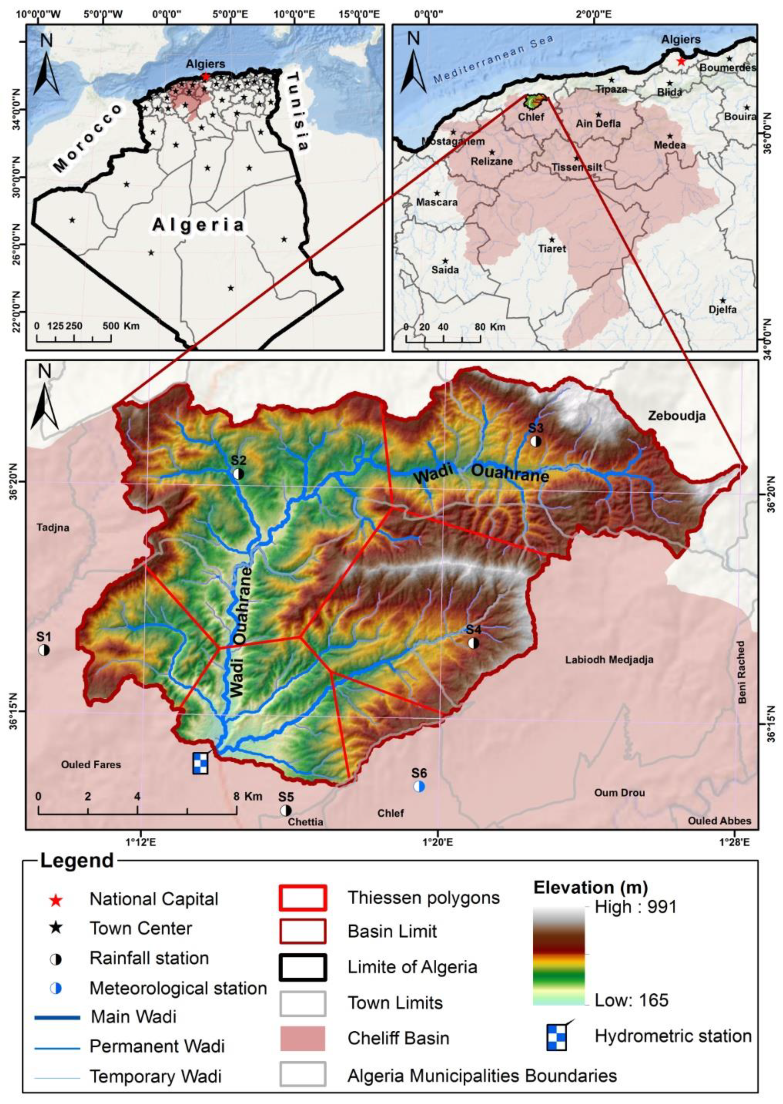
2.1. Study Area and Data Collection

The study area is the Wadi Ouahrane Basin in north Algeria, which is located between 36°00′ and 36°24′ N and between 01°00′ and 01°3′ E. It is a small tributary of the Wadi Cheliff Basin (Figure 1) and has an area of more than 270 km², with a maximum altitude of 991 m a.s.l. and a minimum altitude of 165 m a.s.l.

The Wadi Ouahrane Basin is limited to the east by the basin of Wadi Fodda, to the west by the Wadi Ras Basin, to the north by the Wadi Allala Basin, and to the south by the Wadi Sly Basin. It has a Mediterranean climate, with an annual average rainfall of 333 mm over the period 1972–2018. The mean annual temperature is 18 °C.

The rainfall series used in this study includes data collected monthly at 6 stations (Figure 1 and

Table 1. Rainfall and hydrometric station characteristics.

Stations	Type	ID	Name	Longitude	Latitude	Elevation (m)
S1	H	012201	LARBAT OULED FARES	01°13′56″	36°14′14″	173
S1	R	012201	LARBAT OULED FARES	01°09′18″	36°16′20″	116
S2	R	012224	BOUZGHAIA	01°14′27″	36°20′15″	217
S3	R	012205	BENAIRIA	01°22′28″	36°21′04″	320
S4	R	012221	MEDJAJA	01°20′53″	36°16′39″	487
S5	R	012209	CHETIA	01°15′53″	36°12′56″	108
S6	R	NMO	Airport, Chlef	01°19′28″	36°13′31″	158

H: Hydrometric Station; R: Rainfall Station.

) in the period from 1972 to 2018. These rainfall data were taken from the National Agency of the Water Resources (Agence Nationale des Ressources Hydrauliques–ANRH) and the National Meteorological Office (Office National de Météorologique–ONM). Monthly runoff data from 1972 to 2018 were also collected from ANRH.

With regard to land use/land cover (LULC), changes over the Wadi Ouahrane Basin were evaluated using a remote sensing and geographic information system (GIS). The images were collected for different years, i.e., 1979, 1989, 1999, 2009, and 2017 from the Landsat 2, Landsat 5, Landsat 7, and Landsat 8, with the objective of deriving information on different LULC classes. The multi-temporal remotely sensed images were used for detailed LULC classification. The classified maps for the years 1979, 1989, 1999, 2009, and 2017 are presented in Figure 2. The spatial variation of LULC classes (dense vegetation, moderate vegetation, sparse vegetation, bare soil, and water surface) in different years can be clearly visualized. From

Table 2. Areal coverage details of LULC classes over the Wadi Ouahrane Basin.

Soil Occupation	1979		1989		1999		2009		2017
	Area (km2)	Area (%)	Area (km2)	Area (%)	Area (km2)	Area (%)	Area (km2)	Area (%)	Area (km2)	Area (%)
Dense vegetation	0.00	0.00	0.25	0.09	1.30	0.48	0.17	0.06	0.24	0.09
Moderate vegetation	10.46	3.87	39.87	14.77	56.48	20.92	93.08	34.47	187.80	69.56
Sparse vegetation	86.68	32.10	94.73	35.08	72.52	26.86	96.85	35.87	77.00	28.52
Bare soil	172.86	64.02	135.05	50.02	139.68	51.73	79.90	29.59	4.90	1.81
Water surface	0.00	0.00	0.10	0.04	0.02	0.01	0.00	0.00	0.06	0.02
Total	270	100	270	100	270	100	270	100	270	100

, the temporal changes in individual LULC classes over the Wadi Ouahrane Basin can be noticed. The percentage of basin area under each of these classes during 1979, 1989, 1999, 2009, and 2017 is also presented.

2.2. Analysis Methods

2.2.1. Univariate Indices in Monitoring of Meteorological and Hydrological Drought

In this study, the Thiessen polygons method was first applied to compute the mean monthly areal rainfall in the study area, which was then used to find SPI. SPI and SRI were first proposed by McKee et al. [34] and Shukla and Wood [35], respectively, and are widely used to assess meteorological (SPI) and hydrological (SRI) droughts. If X_w represents the total precipitation (runoff) over a period of w previous months, by fitting a suitable distribution such as the gamma distribution of the X_w time series, $u_w=F_{x_w\left(x_w\right)}$, a marginal cumulative distribution function (CDF) is obtained. Then the SPI (SRI) is transformed to normality by applying the inverse CDF for the standard normal distribution or ${\phi }^{-1}\left(u_w\right)$. In other words, the distribution of the SPI or SRI time series at any timescale w is described by a standard normal variable (mean zero and standard deviation of 1).

Although the method of calculating SPI and SRI seems logical in appearance, it has its drawbacks. For example, there may be significant autocorrelation in the observations, leading to a skewed probabilistic fit. This problem is exacerbated for longer timescales, because the successive samples have more overlap. To solve this problem, according to Kao and Govindarajo [36], a modified SPI and SRI were used in this study. The modification is in normalizing the precipitation or runoff series ending in each month of the year separately, so that SPI and SRI both have zero mean and unit standard deviation for any month of the year, and autocorrelation within each subseries is greatly reduced [36]. X_w is grouped by its ending month to create a new dataset $X_w^{\mathrm{month}}$, in which month represents one of the months of January, February, …December. In this way, $X_1^{\mathrm{Jan}}$ represents January rainfall and $X_5^{\mathrm{Aug}}$ represents the total five-month rainfall from April to August, and thus samples in each $X_w^{\mathrm{month}}$ dataset are collected annually without overlapping as long as w ≤ 12. By fitting the distribution function to each group separately, SPI^mod was calculated similarly to the original SPI from the following equation:

$${\mathrm{SPI}}_w^{\mathrm{mod}}={\phi }^{-1}\left(u_w^{\mathrm{month}}\right)={\phi }^{-1}\left(F_{X_w^{\mathrm{month}}}\left(u_w^{\mathrm{month}}\right)\right)$$

(1)

Precipitation margins (univariate cumulative distribution functions) $\left\{u_1,u_2\dots u_{12}\right\}$ with different timescales from 1 to 12 months can be generated by the SPI^mod method. u₁ shows last month’s rainfall status (u₁ is important for detecting the onset of drought) and u₁₂ represents last year’s rainfall status (important for diagnosing long-term droughts). It should be noted that none of the u_i can completely reflect the information of the other u_j, and each single u_i can only reflect a partial view of the meteorological drought as a cross-timescale phenomenon. The same process can be applied to generate runoff indices based on 1 to 12 month timescale modified SRI, {v₁, v₂, …, v₁₂}, which each give a partial representation of hydrological drought.

2.2.2. Drought Definition and Characteristics

Table 3. Classification of drought based on SPI (SRI).

SPI Values	Drought Category
2.00 or more	Extremely wet
1.50 to 1.99	Very wet
1.00 to 1.49	Moderately wet
0 to 0.99	Near normal
−0.99 to 0	Mild drought
−1.00 to −1.49	Moderate drought
−1.50 to −1.99	Severe drought
−2.00 or less	Extreme drought

shows the classification of drought severity based on SPI values, which can be used also for the SRI.

In this study, according to the recommendation of Loucas and Vasiliads [37], meteorological (resp. hydrological) drought events were defined as periods in which drought index values (such as the modified SPI or resp. SRI at some given timescale w) are less than zero. Some other researchers, such as Xiao [38], Shiau and Modarres [39], and Mirabbasi et al. [40] have defined drought in the same way. A period of drought begins when the drought index value is consistently negative (for two months or more) [34]. This period ends when the index returns to positive values. Therefore, each drought event has a period of time that is defined by its onset and end, which is called drought duration. Drought severity is defined as accumulated index deficit, which indicates the amount of moisture deviation from normal during a determined period [41]. Acute water resource problems during droughts are generally associated with long-term and severe events.

2.2.3. Copula Functions

Copulas are a flexible way to create probability distributions with different margin functions. In essence, copula is a function that combines any specified margins of univariate distribution functions to form a two- or multi-variate distribution function. Copulas are multivariate distribution functions whose one-dimensional margins are uniform over the range [0,1]. Sklar [42] showed theoretically how any univariate distribution functions can be combined with any copula to form valid multivariate distributions. Although copula theory was proposed for general dimensions (2 or more), the complexity of the joints increases rapidly with an increasing number of variables. Therefore, many researchers use empirical copulas in multivariate analysis (especially in dimensions much higher than 2). The concept of empirical copulas is in fact similar to the concept of graph positional formulas used in the univariate statistical analysis. When a large enough sample is available, empirical copulas can be used to create non-parametric joint empirical probability distributions that are computationally efficient [43,44].

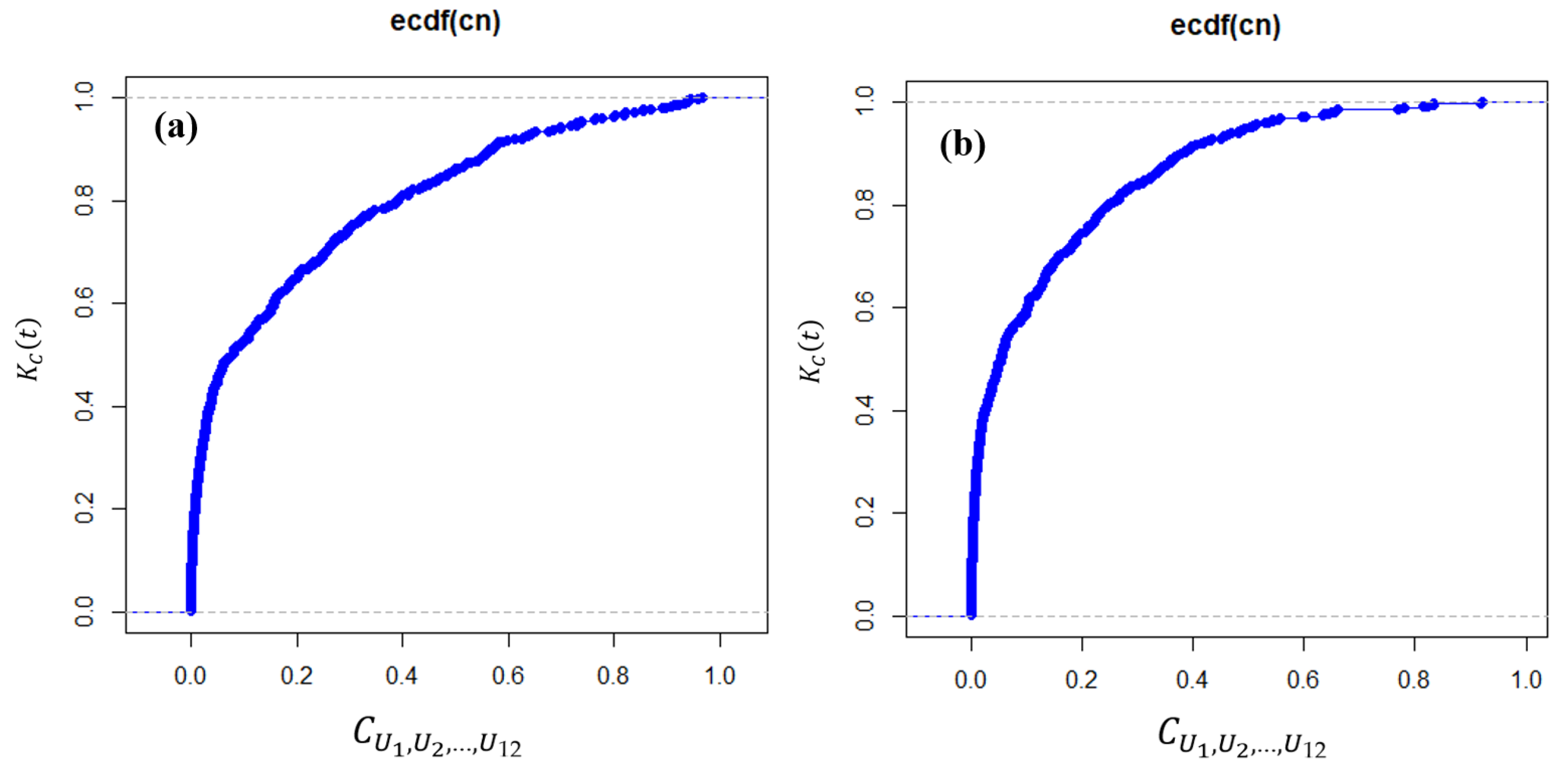
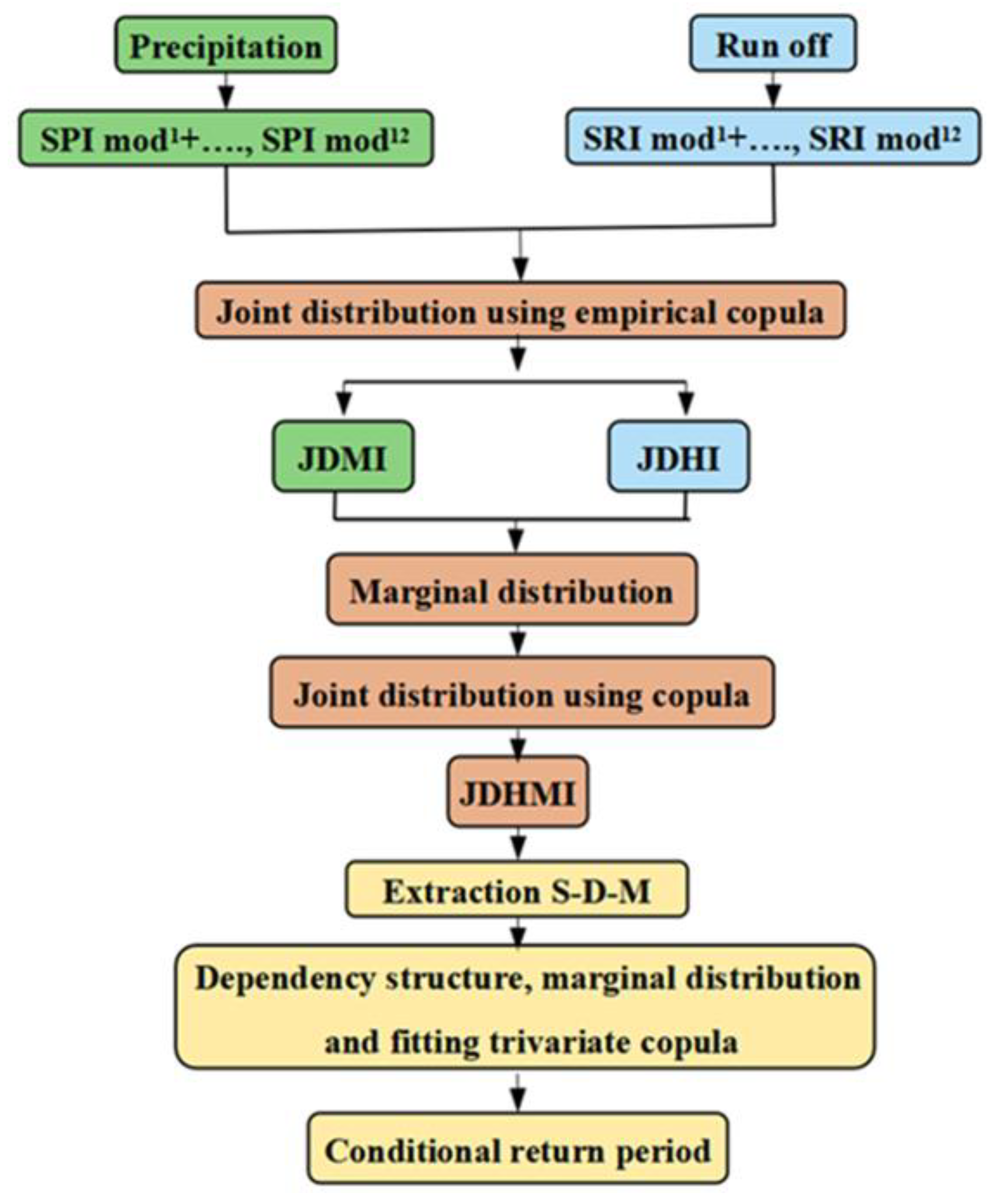
2.2.4. Joint Deficit Index (JDI)

Kao and Govindarauo [36] defined the joint drought index (JDI) using the joint distribution function to provide a scientific description of the general drought condition across a set of timescales (1 to 12 months). In order to create the JDI, parametric or empirical copulas can be used to create the dependency structure of the u₁, u₂, …, u₁₂ (or v₁, v₂, …, v₁₂) set. However, due to the mathematical complexity of 12-dimensional parametric copulas, Kao and Govindaraju [36] used empirical joints for this purpose. To specify the dependence structure encoded in a copula, either parametric or non-parametric approaches can be used. However, in a higher-dimensional setting, the non-parametric approach has an advantage over the parametric one, given the complexity of parameter estimation as well as the strong assumptions that have to be made in the parametric approach. Empirical Copula [45] with dependence structure defined by independent rank transformations of the samples in each of the dimensions of the multivariate data space, provides a non-parametric alternative to circumvent the above issues associated with the parametric approach. According to the definition of Empirical Copula, if two multivariate samples have identical rank structures, their Empirical Copulas are the same [46]. The choice of u₁, u₂, …, u₁₂ in forming high-dimensional copulas increases the complexity of the dependency model [47]. However, because the duration of droughts shows wide time variations, droughts can only be well described by considering different periods (from 1 to 12 months). In addition, this structure allows for a month-by-month assessment of future conditions. Kao and Govindaraju [36] did not consider timescales longer than 12 months (w > 12) because they observed that the samples used will overlap, and even after applying the modified SPI process, the results could be distorted. Therefore, in this study, only 12 modified SPIs were considered to create the joint deficit meteorological index (JDMI), and the corresponding modified SRIs were used to create the joint deficit hydrological index (JDHI), both special cases of the JDI concept.

A copula is actually the cumulative probability $P\left[U_1\le u_1,\dots ,U_{12}\le u_{12}\right]=t$ of the marginals of the u₁, u₂, …, u₁₂ sample. As each margin indicates the conditions of moisture deficiency for each given period of time, the conditions of joint deficit are determined by t. Clearly, a smaller cumulative probability indicates drier conditions (drought on different time scales), and a larger value indicates wetter conditions. Assuming t reflects the severity of the combined drought, knowing the probability of events occurring with joint values less than or equal to t (i.e., events drier than a certain threshold) will be very beneficial. For this purpose, the definition of the joint distribution function is used, because the joint distribution function is in fact the cumulative probability $K_C\left(t\right)=P\left[C_{U_1,U_2,\dots ,U_{12}}\left(u_1,u_2,\dots ,u_{12}\right)\right]t$. The special advantage of using K_C is that it allows a single probabilistic criterion for joint deficit conditions to be calculated, which can be interpreted as an indicator of combined drought. In fact, K_C is the joint CDF. Figure 3 shows the distribution function of K_C in different values of $C_{U_1,U_2,\dots ,U_{12}}$ joints for the rainfall (Figure 3a) and runoff (Figure 3b) of the study area.

Therefore, the joint deficit index (JDI) was defined similar to the SPI (SRI) [47].

$$\mathrm{JDI}={\phi }^{-1}\left(K_C\right),$$

(2)

Similar to SPI (SRI), a positive JDI (K_C > 0.5) indicates a general wet condition, a negative JDI (K_C < 0.5) indicates a general dry condition, and JDI = 0 (K_C = 0.5) indicates a normal condition. Since JDI is inverted on a normal scale (similar to SPI (SRI)), the classification of droughts based on the SPI (SRI) (Table 3) can also be applied to the JDMI (JDHI). The most important character of JDI is the evaluation of general joint conditions based on the structure of dependence of deficiency indices with different time periods.

2.3. Parametric Copula

In general, copula functions are divided into parametric and non-parametric categories. Parametric copulas are preferred, at least over 2 or 3 dimensions, since copula fitting with the input data makes it possible to extrapolate beyond its range, which is a limitation for non-parametric copulas. The copula parameters represent the intensity of the dependence of the variables and have a certain mathematical relationship with it. Due to the use of different parameters in different parametric copulas, the results will also be different [48]; the best copula type to use for a given data type can be determined using goodness of fit tests. Among the copula functions, the Archimedean and Elliptical copula family of functions are the most widely used.

Table 4. Parametric copulas used by the Archimedean and elliptical families.

Copulas	Bivariate Copula C (u, v)	Parameters
	Elliptical copulas
Student’s t	${{\displaystyle \int }}_{-\infty }^{t_{\theta }^{-1}\left(u\right)}{{\displaystyle \int }}_{-\infty }^{t_{\theta }^{-1}\left(v\right)}\frac{1}{2\pi \sqrt{1 - r^2}}{\left\{1+\frac{x^2 - 2rxy + y^2}{\theta \left(1 - r^2\right)}\right\}}^{\frac{-\theta + 2}{2}}\mathrm{dxdy}$ $t_{\theta }\left(x\right)={{\displaystyle \int }}_{-\infty }^x\frac{\Gamma \left(\frac{\theta + 1}{2}\right)}{\sqrt{\pi \theta }\Gamma \left(\theta /2\right)}{\left(1+y^2/\theta \right)}^{\frac{-\theta + 1}{2}}dy$	$\theta >2,r\in \left(0,1\right]$
Gaussian	${\Phi }_2\left({\Phi }^{-1}\left(u\right),{\Phi }^{-1}\left(v\right),\rho \right)$	$-1\le \rho \le 1$
	Archimedean copulas
Clayton	${\left(u^{-\theta }+v^{-\theta }-1\right)}^{-1/\theta }$	$\theta \in {\displaystyle \cup }\left(0,\infty \right)$
Frank	$\frac{-1}{\theta }\log \left[1+\frac{\left(e^{-\theta u} - 1\right)\left(e^{-\theta v} - 1\right)}{e^{-\theta } - 1}\right]$	$\theta \in {\displaystyle \cup }\left(0,\infty \right)$
Joe	$1-{\left[{\left(1-u\right)}^{\theta }+{\left(1-v\right)}^{\theta }-{\left(1-u\right)}^{\theta }{\left(1-v\right)}^{\theta }\right]}^{1/\theta }$	$\theta \in {\displaystyle \cup }\left(0,\infty \right)$

shows the types of parametric copulas considered and their equations and parameters.

2.4. Estimation of Parameters and Goodness of Fit Test

In the present study, the maximum likelihood (ML) method was used to estimate the parameters in marginal distribution. The Akaike (AIC) [49] and the Bayesian (BIC) [50] are the most commonly used information criteria for selecting the best model from all available models used. A model is better with a smaller AIC (or BIC). The basis of the AIC is the Kullback–Leibler distance in information theory, while the basis of BIC is the integrated neighborhood in Bayesian theory [51].

One of the advantages of using copula functions in multivariate distributions is that they take into account the correlation between variables and in fact do not require the independence of the variable, but even these functions take into account the structure of the correlation between the variables. When estimating the copula function, the value of the correlation coefficient must be specified. Three coefficients—Kendall correlation, Spearman coefficient, and Pearson coefficient—were used for this purpose [43,50].

In copulas, the Maximum Pseudo-Likelihood (MPL) method was used to estimate the parameters, and the AIC, BIC, and Cramér–von Mises test statistic were used for the goodness of fit test [52].

In the current study, the copula was selected based on the P value, which was obtained from the bootstrap method [53]. The higher the P value, the better the copula.

In addition to the numerical approach, Chi plot and Kendall plot were used to graphically represent the degree of fit, all of which are contained in the copula package in R software [54].

2.5. Conditional Return Period

The copula function interprets the dependency structure between drought characteristics very well. In this study, we used three variables—Severity-Duration-Magnitude (S-D-M)—for the conditional return period, as follows [52]:

$$P\left(S\le s,D\le d\vee M\ge m\right)=\frac{P\left(S\le s,D\le d,M\ge m\right)}{P\left(M\ge m\right)}=\frac{C_1\left(s,d\right)-C_2\left(s,d,m\right)}{1-F_m\left(m\right)}=\frac{C_1\left(s,d\right)-C_2\left(C_1\left(s,d\right),F_m\left(m\right)\right)}{1-F_m\left(m\right)},$$

(3)

The methodology steps are presented in Figure 4.

3. Results

3.1. Calculation of Univariate Drought Indices and Fitting of Marginal Distribution Functions

Table 5. Goodness of fit test statistics on SPI^mod and SRI^mod.

	Distribution	Statistics	Evaluation Index
SPImod (1,2, …, 12)	Gamma	K–S = 0.16; CM = 4.79; A–D = 27.37	AIC = 4656; BIC = 4665
SRImod (1,2, …, 12)	Log-normal	K–S = 0.15; CM = 1.26; A–D = 7.83	AIC = −788; BIC = −780

represents the results of goodness of fit tests at the 5% significance level for $X_w^{\mathrm{month}}\left(W=1,2,\dots 12\right)$ for precipitation and runoff based on Kolmogorov–Smirnov (K–S), Cramér–von Mises (CM), Anderson–Darling (A–D), AIC, and BIC.

The best fitted model on modified $X_w^{\mathrm{month}}$ (w = 1, 2, …, 12) for precipitation and runoff was determined to be the gamma and log-normal distribution, respectively (Table 5). These were used for transforming the SPI and SRI series to approximately follow standard normal distributions.

3.2. Correlation Analysis of Two Variables of Modified Rainfall and Runoff Indices

Spearman rho coefficient, Kendall tau, and Pearson coefficient correlation were used to evaluate the correlation between rainfall and runoff. In the three methods, the correlation coefficient was significant. Here the Spearman rho correlation coefficient between $\left\{u_1^{\mathrm{mod}},u_2^{\mathrm{mod}},\dots ,u_{12}^{\mathrm{mod}}\right\}$ (precipitation marginal distribution functions) and $\left\{v_1^{\mathrm{mod}},v_2^{\mathrm{mod}},\dots ,v_{12}^{\mathrm{mod}}\right\}$ (runoff margin distribution functions) is presented in

Table 6. Spearman correlation coefficient between u_i, u_j (upper triangle) for precipitation marginal and v_i, v_j (lower triangle) for runoff marginal cumulative distribution functions (r_ij = r_ji).

	i	$\mathrm{Spearman}\prime \mathrm{s} r_{ij} \mathrm{between} u_i^{\mathrm{mod}}$$\mathrm{and} u_j^{\mathrm{mod}}$
j		1	2	3	4	5	6	7	8	9	10	11	12
Spearman’s ri,j between vimod and vjmod	1		0.84	0.70	0.57	0.42	0.28	0.17	0.07	0.00	0.00	0.08	0.19
	2	0.87		0.90	0.77	0.64	0.49	0.35	0.24	0.15	0.11	0.16	0.26
	3	0.76	0.92		0.92	0.81	0.68	0.53	0.41	0.30	0.24	0.24	0.32
	4	0.65	0.83	0.94		0.93	0.83	0.70	0.56	0.44	0.36	0.33	0.35
	5	0.53	0.71	0.84	0.94		0.94	0.83	0.71	0.58	0.47	0.41	0.40
	6	0.42	0.58	0.72	0.85	0.94		0.94	0.84	0.71	0.58	0.49	0.45
	7	0.34	0.48	0.62	0.75	0.86	0.95		0.94	0.83	0.71	0.59	0.51
	8	0.28	0.40	0.52	0.65	0.77	0.87	0.95		0.94	0.82	0.70	0.60
	9	0.25	0.35	0.46	0.56	0.68	0.79	0.88	0.96		0.93	0.81	0.70
	10	0.24	0.33	0.41	0.50	0.61	0.71	0.81	0.90	0.96		0.93	0.82
	11	0.26	0.33	0.40	0.47	0.56	0.65	0.74	0.83	0.91	0.97		0.93
	12	0.31	0.36	0.41	0.47	0.54	0.62	0.70	0.79	0.86	0.93	0.97

.

In this table, the values of the Spearman correlation coefficient (r_ij) are shown in pairs for the marginal distribution functions ${\mathrm{SPI}}_W^{\mathrm{mod}}$ and ${\mathrm{SRI}}_W^{\mathrm{mod}}$ for w = 1, 2, …, 12. For precipitation marginal distributions as shown in Table 5, the short-term marginals $u_1^{\mathrm{mod}}$ have a high correlation with $u_2^{\mathrm{mod}}$, which is equal to 0.84. The correlation coefficient decreases with increasing time window i (when i ≥ 6, the correlation between $u_1^{\mathrm{mod}}$ and $u_i^{\mathrm{mod}}$ becomes less than 0.13). The long-term margin distribution function $u_{12}^{\mathrm{mod}}$ has a high correlation with $u_j^{\mathrm{mod}}$ at j > 5, and the correlation coefficient decreases when the time window is shorter (less than 5). These findings are consistent with the results of Kao and Govindaraju [55] for calculating the joint deficit index using precipitation and runoff data. $u_1^{\mathrm{mod}}$ shows last month’s rainfall status (important for identifying ongoing droughts), and $u_{12}^{\mathrm{mod}}$ shows last year’s rainfall status (important for identifying long-term droughts). Although not well correlated with each other, none of them can be ignored.

Table 5 also shows that no single $u_1^{\mathrm{mod}}$ ($v_1^{\mathrm{mod}}$) can represent other time windows alone, and therefore each $u_1^{\mathrm{mod}}$ ($v_1^{\mathrm{mod}}$) represents a small fraction of meteorological (hydrological) drought. Similar observations can be made about runoff. Compared to rainfall marginal distribution functions, a high level of temporal correlation is observed for runoff, as expected. However, similar to precipitation, a single time window cannot be used to show the total drought situation.

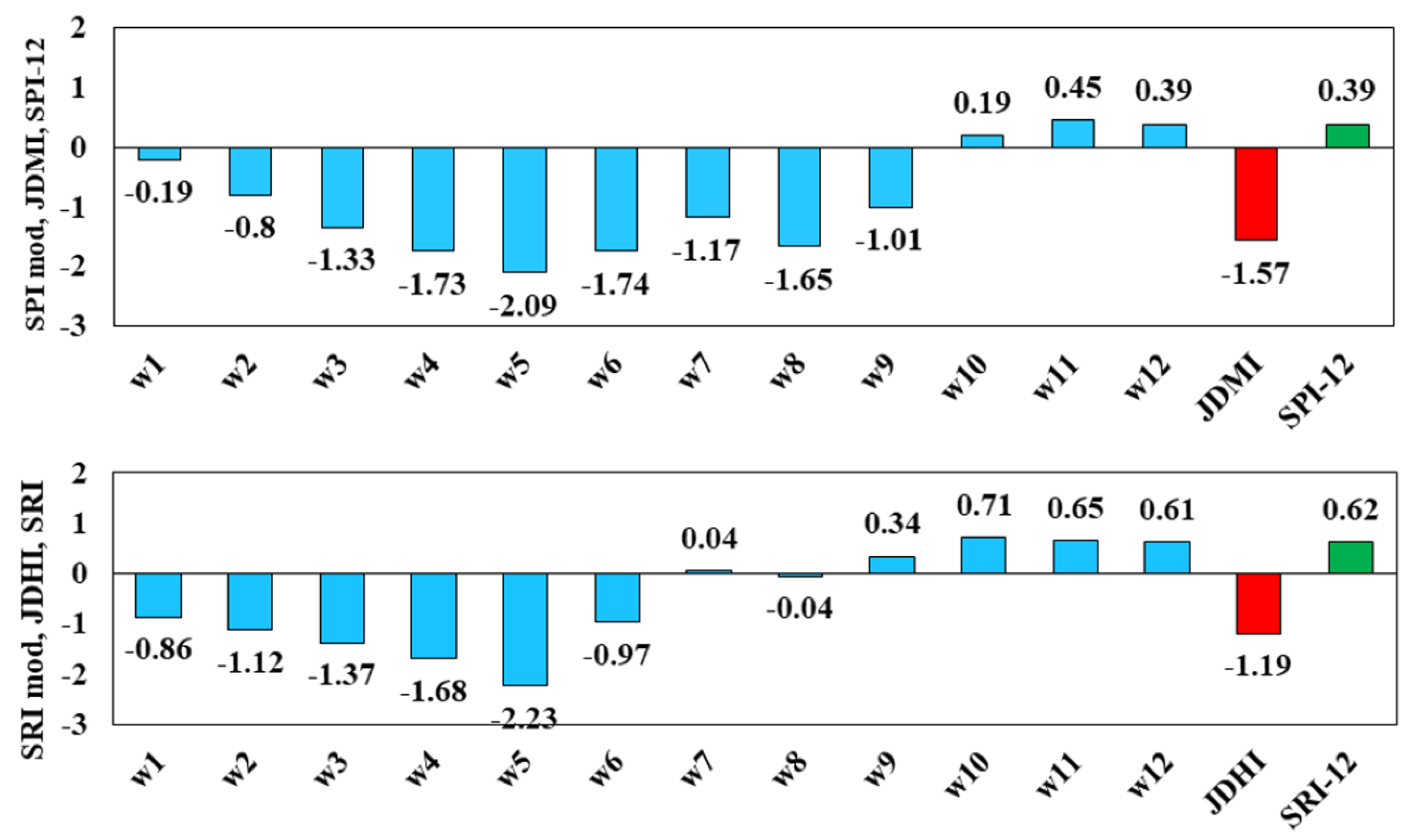
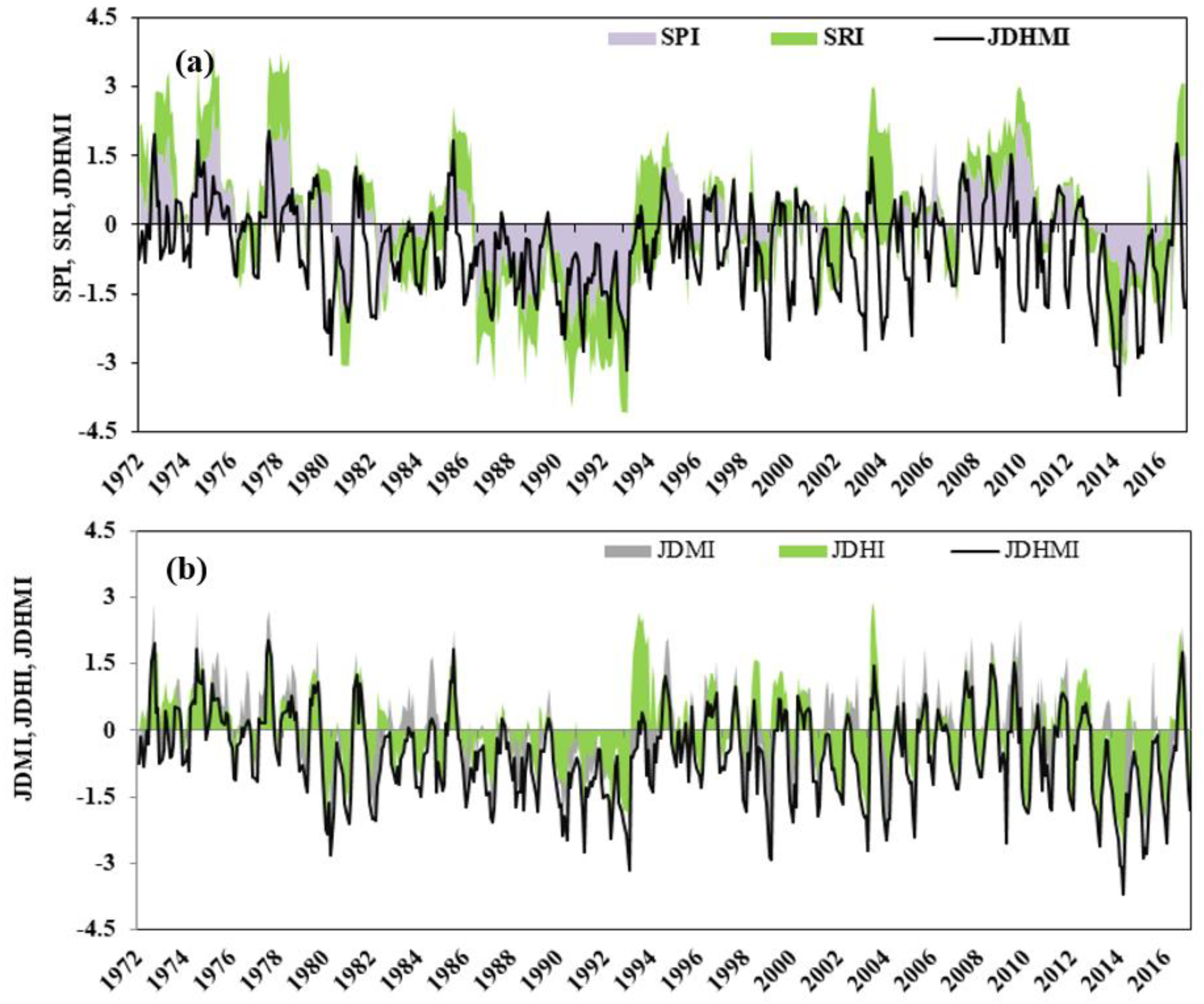
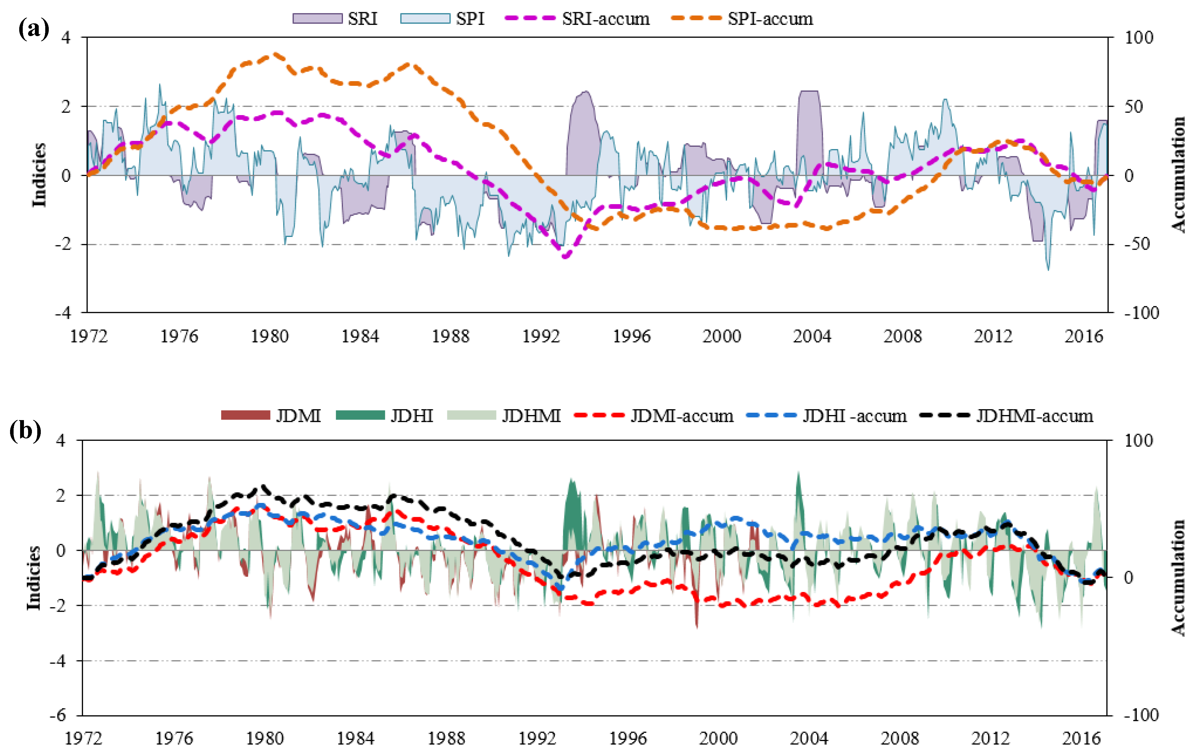
3.3. Comparison of Multivariate Indices with Univariate Indices

After examining the correlation between the variables in Section 3.2, JDMI and JDHI indices were calculated. Figure 5 shows a comparison of the values of SPI, SPI^mod, and JDMI for precipitation and SRI, SRI^mod, and JDHI for runoff in October 1982 as examples. The rate of change in precipitation during this period (October 1982 in the past 12 months) varies from 0 mm to 88 mm, and runoff from 0 to 0.392 m³/s. This month was selected because, in this period, the joint deficit indices (JDHI, JDMI) showed severe and extreme drought, and thus it is a good example to show the efficiency of hydrometeorological indices.

As described in the methodology, JDMI (JDHI) is obtained from the combination of ${\mathrm{SPI}}_1^{\mathrm{mod}}$–${\mathrm{SPI}}_{12}^{\mathrm{mod}}$ (${\mathrm{SRI}}_1^{\mathrm{mod}}$–${\mathrm{SRI}}_{12}^{\mathrm{mod}}$) using the empirical Kendall copula function. According to this figure, the SPI value is 0.39 while the JDMI is −1.57. In this case, the interpretation of drought in such a situation is more complex. This is because the precipitation rate has changed greatly over the last 12 months. The univariate index is not able to accurately define the drought situation. However, the JDMI shows the state of the meteorological drought based on the structure of the dependence between the precipitation of the last 12 months. In other words, for October 1982, while the precipitation rate was normal for the last 12 months on the whole, the lack of precipitation in the previous months (w₁, w₂, …, w₉) was so severe that it negatively affected the JDMI index (severe drought). The case for hydrological drought is similar to that for meteorological drought. Thus, the SRI value in October 1982 was 0.62, indicating wet conditions, while the calculated JDHI value was −1.19, indicating drought.

3.4. Hydro-Meteorological Joint Deficit Drought Index

Using the parametric copula function, two indices, JDMI and JDHI, were joined, and JDHMI was obtained. To compare the reliability of a JDHMI composite index with other univariate and multivariate indices, the JDHMI time series was compared with JDMI, JDHI, SRI, and SPI (Figure 6). As shown, JDHMI, unlike SPI and SRI, is based on the common probability ^mod of all SPI^mods and SRI^mods and provides a comprehensive overview of drought conditions. JDHMI fluctuations are similar to those of JDMI and JDHI when these are the same sign, but mediates between them during some transition periods when they have opposite signs. For JDMI or JDHI individually, which use SPI^mod or SRI^mod alone, a comprehensive view of the prevailing hydro-meteorological situation in the region cannot be achieved, due to not considering the simultaneous effects of precipitation and runoff in a drought. Therefore, the composite index is able to reflect the simultaneous hydrological and meteorological behavior well, and it can be inferred that JDHMI can present the probability of a common hydrological and meteorological deficit situation more accurately and realistically than univariate and multivariate precipitation-based indicators or runoff alone.

In addition, with the aim of comparing the performance of the composite index and its similarity with the indices derived from it, Figure 7 is presented. Figure 7a shows that the SPI and SRI time series cumulative values have an uptrend from 1972 to 1980 (wet) and have been lower since 1991, after a severe and prolonged drought in the later 1980s. Multivariate and composite indices derived from empirical and parametric copulas (Figure 7b) also reflect the behavior of univariate indices. Two multivariate indices (JDMI, JDHI) show similar behavior to meteorological and hydrological indices, but the composite index derived from JDMI and JDHI is a combination of hydrological and meteorological drought behavior in the region, which reflects the effect of two variables.

3.5. Correlation between Composite, Multivariate, and Univariate Indices

The degree of consistency between univariate, multivariate, and composite indices was assessed using the correlation coefficient (CC). In particular, the CC measures the linear relationship between two time series. High values of CC indicate a high agreement between multivariate indicators. According to

Table 7. Correlation coefficient between indices.

Indices	SPI-12	SRI-12	JDMI	JDHI	JDHMI
SPI-12	1.00	0.52	0.60	0.32	0.51
SRI-12	0.52	1.00	0.28	0.52	0.58
JDMI	0.60	0.28	1.00	0.61	0.89
JDHI	0.32	0.52	0.61	1.00	0.86
JDHMI	0.51	0.58	0.89	0.86	1.00

, there is high correlation between JDHMI and SPI, SRI, JDMI, and JDHI, and the correlation range is between 0.51 and 0.86. Univariate and multivariate indices contain a percentage of hydro-meteorological drought change information, but the composite index (JDHMI) is based on a fuller set of precipitation and runoff information of the region and combines the effects of two types of droughts.

Generally, correlation coefficients between the JDHMI and single drought indices are mostly over 0.5, indicating that the JDHMI can reflect the comprehensive meteorological and hydrological drought properties simultaneously. This suggests that the copulas can represent the complicated and nonlinear relationship among different drought indices to yield a satisfactory combined drought index. In addition, the margin-free characteristics are completely preserved by the copula function when constructing the joint distribution function.

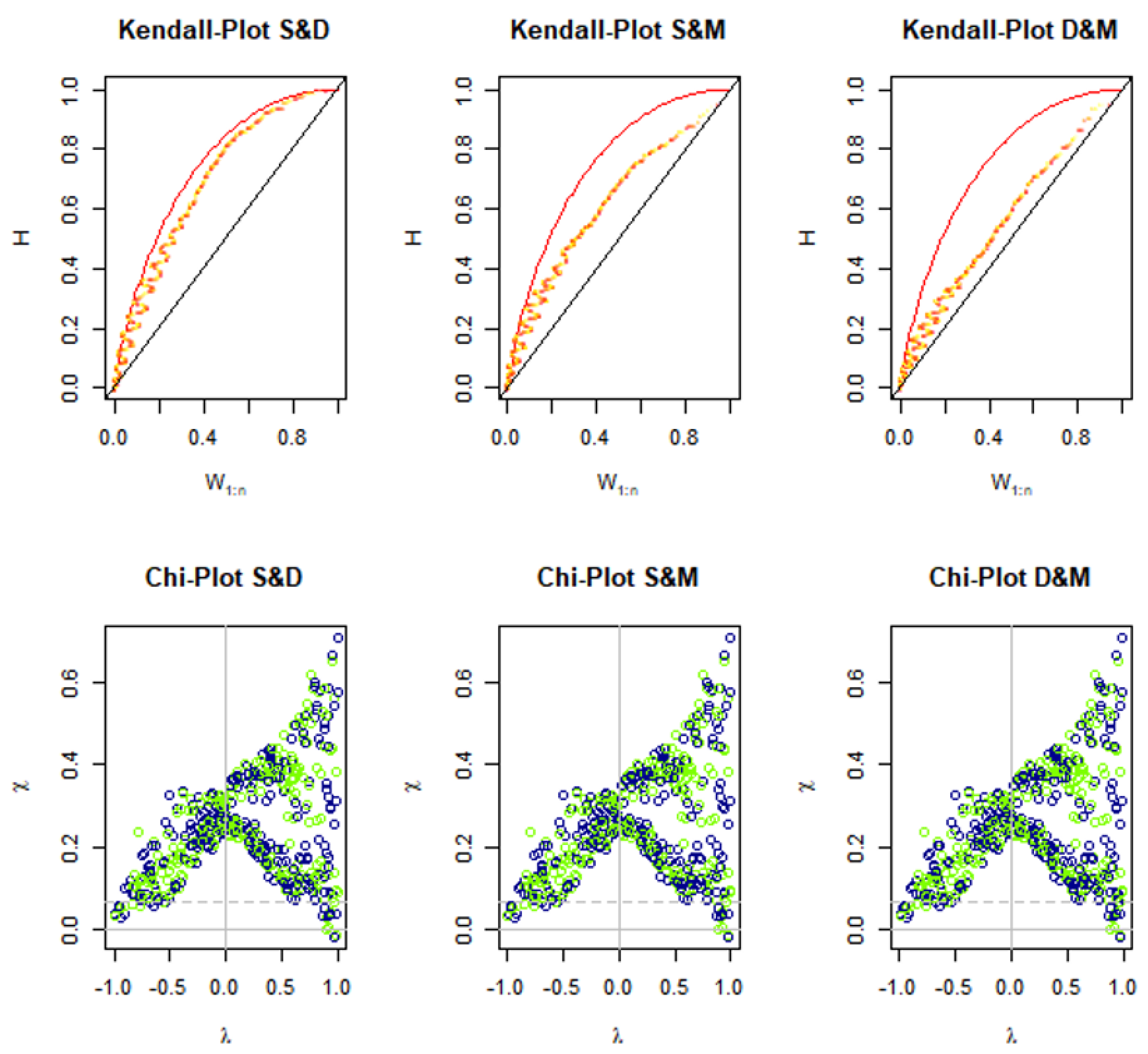
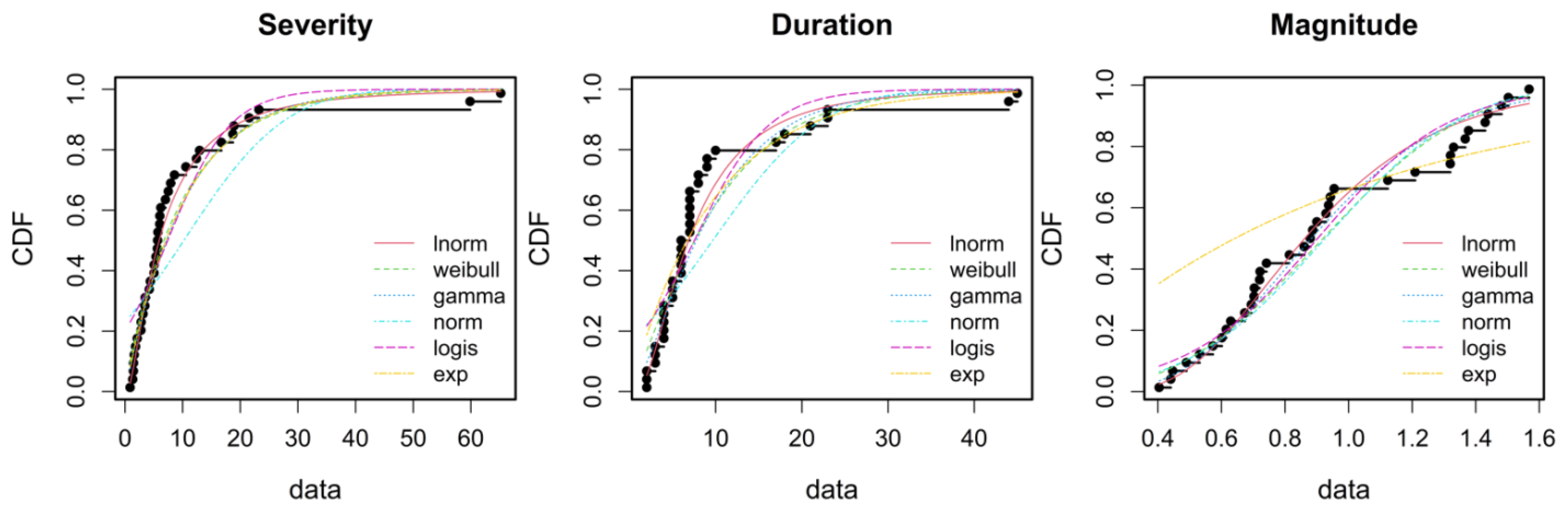
3.6. Correlation Structures of Drought Variables and Fitting of Marginal Functions

Based on the methodology of Section 2.2.1, drought severity, duration, and magnitude were extracted from JDHMI. Their descriptive characteristics are presented in

Table 8. Statistical characteristics of hydro-meteorological drought (JDHMI) variables.

	Characteristics	Value
	Number of months less than zero	261
Maximum	severity	65.19
	duration	45
	magnitude	1.57
Average	severity	10.19
	duration	9.65
	magnitude	0.93
Minimum	severity	0.88
	duration	2
	magnitude	0.41

. According to the results, 261 events of hydro-meteorological drought occurred in the study area, with maximum severity, duration, and magnitude of 65, 45 months, and 1.57, respectively. The average severity of hydro-meteorological drought in the study area was 10.19, with a duration of 9 months and a magnitude of 0.93. The study area has a minimum drought duration of 2 months, with a magnitude of 0.88 and a magnitude of 0.41.

Figure 8 shows the chi-plot and Kendall plot of the variables extracted from the JDHMI. These two graphs are a tool to study the structure of the correlation between two variables. In the Kendall plot (Figure 8, top), two variables are correlated when the event points deviate from the diagonal line. The points above the diagonal line indicate a positive correlation, and the points below the diagonal line indicate a negative correlation [56]. Based on the results of the Kendall plot, a strong deviation from the diagonal line is seen, which indicates a positive correlation between the variables of severity, duration, and magnitude of drought in the study area. The two variables can be considered independent when most events fall within the chi-plot confidence range (Figure 8) [43,57]. In the chi plot, a strong deviation from the confidence band was observed for all points, and all points are far from the chi plot confidence range. In addition, most of the studied variables are higher than the mean (positive lambda values).

Table 9. Goodness of fit test of marginal distribution function on hydro-meteorological drought characteristics.

Indices	Functions	Parameters	K–S Test		Evaluation Index
			S	p
Severity	Weibull	λ = 0.95, k = 9.88	0.05	0.15	AIC = 249.55; BIC = 252.77
	Gamma	α = 1.05; β = 0.10	0.07	0.17	AIC = 249.72; BIC = 252.94
	Log-normal	µ = 1.77; σ = 0.99	0.06	0.10	AIC = 239.85; BIC = 243.07
	Normal	µ = 10.19; σ = 13.80	0.02	0.28	AIC = 303.27; BIC = 306.49
	Logistic	λ = 7.40; k = 5.40	0.05	0.23	AIC = 285.31; BIC = 288.53
	Exponential	λ = 0.098	0.08	0.17	AIC = 247.78; BIC = 249.39
Duration	Weibull	λ = 1.1, k = 10.30	0.08	0.21	AIC = 243.96; BIC = 247.19
	Gamma	α = 1.61; β = 0.17	0.06	0.22	AIC = 241.30; BIC = 244.52
	Log-normal	µ = 1.92; σ = 0.77	0.14	0.17	AIC = 231.80; BIC = 235.02
	Normal	µ = 9.64; σ = 9.98	0.15	0.31	AIC = 143.86; BIC = 146.38
	Logistic	λ = 7.52; k = 4.31	0.11	0.22	AIC = 267.30; BIC = 270.52
	Exponential	λ = 0.10	0.09	0.19	AIC = 243.74; BIC = 245.35
Magnitude	Weibull	λ = 2.94, k = 1.04	0.09	0.14	AIC = 28.48; BIC = 31.70
	Gamma	α = 7.01; β = 7.67	0.091	0.14	AIC = 27.19; BIC = 30.42
	Log-normal	µ = −0.14; σ = 0.38	0.11	0.14	AIC = 27.32; BIC = 30.54
	Normal	µ = 0.93; σ = 0.34	0.09	0.14	AIC = 30.36; BIC = 33.58
	Logistic	λ = 0.90; k = 0.21	0.08	0.15	AIC = 33.42; BIC = 36.65
	Exponential	λ = 1.08	0.05	0.35	AIC = 70.32; BIC = 71.93

shows the marginal functions of the S-D-M variables, the function parameters, and the goodness of fit test based on AIC, SBC (Schwarz criterion), and K–S statistics. The AIC is computed based on the Kullback–Leibler distance from information theory, and the SBC is based on the integrated likelihood from Bayesian theory, which both impose an appropriate penalty on the average of the log-likelihood of models estimated given the number of coefficients estimated. A model with the lowest AIC and SBC values is the one most likely to be the best [43,44]. In the K–S test, if the p-value was more than 0.05, the null hypothesis that the drought distribution follows the candidate parametric one is accepted at 5% level of significance.

The AIC and SBC values and K–S test results are presented in Table 9. Based on the results, the normal, log-normal, and gamma functions are the best functions on marginal distribution of the variables of drought severity, duration, and magnitude, respectively. Figure 9 shows the CDF of the functions on the variables.

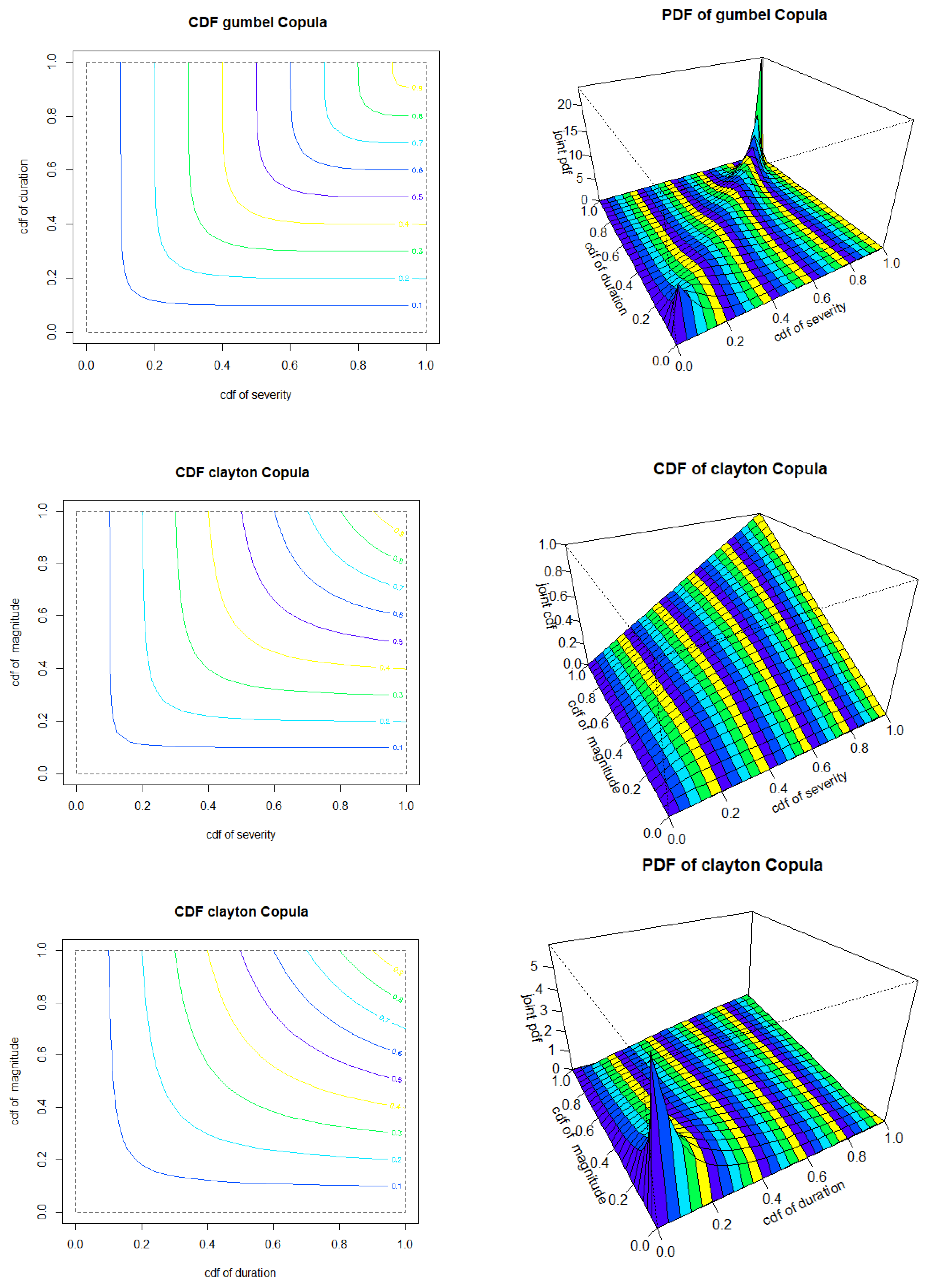
3.7. Fitting of Copula Functions to a Pair of Hydro-Meteorological Drought Variables

After proving the correlation between the variables and selecting the best marginal distribution function on S-D-M, parametric copula distribution functions of the Archimedean and elliptical families were used to construct the three-variable joint distribution functions. The best Coppola was selected based on Sn and ML statistics. According to

Table 10. The results of the optimal copulas and parameters for the S-D-M.

Variables	Function	Sn	Parameter	p-Value	ML
Severity-Duration	Frank	0.03	13.93	0.76	33.59
	Joe	0.022	5.30	0.95	34.83
	Clayton	0.060	3.65	0.053	26.25
	Normal	0.081	0.94	0.011	38.59
	T	0.080	0.94	0.01	38.59
	Gumbel	0.048	4.05	0.95	38.63
Severity-Magnitude	Frank	0.064	5.67	0.015	12.3
	Joe	0.049	1.64	0.22	4.54
	Clayton	0.04	2.19	0.78	17.22
	Normal	0.08	0.70	0.019	12.46
	T	0.04	0.70	0.08	12.52
	Gumbel	0.04	1.66	0.55	8.14
Duration-Magnitude	Frank	0.04	2.51	0.67	3.18
	Joe	0.10	1.20	0.01	0.99
	Clayton	0.10	0.89	0.461	4.58
	Normal	0.032	0.40	0.12	3.30
	T	0.038	0.41	0.11	3.40
	Gumbel	0.039	1.22	0.29	1.85
Severity-Duration-Magnitude	Frank	0.046	5.30	0.18	25.04
	Joe	0.04	1.63	0.27	12.53
	Clayton	0.032	1.77	0.83	29.28
	Normal	0.02	0.68	0.22	26.28
	T	0.050	0.67	0.97	30.42
	Gumbel	0.081	1.62	0.03	18.98

, for S-D the Gumbel function, S-M and D-M for the Clayton function, and the S-D-M for the t function were the most suitable. CDF and PDF (Probability density function) of the appropriate copulas of the variables used are shown in Figure 10.

In Figure 11, the three-dimensional plot (cloud plot) on the left shows the probability of the three variables using the t copula, and the diagram on the right shows the cumulative distribution.

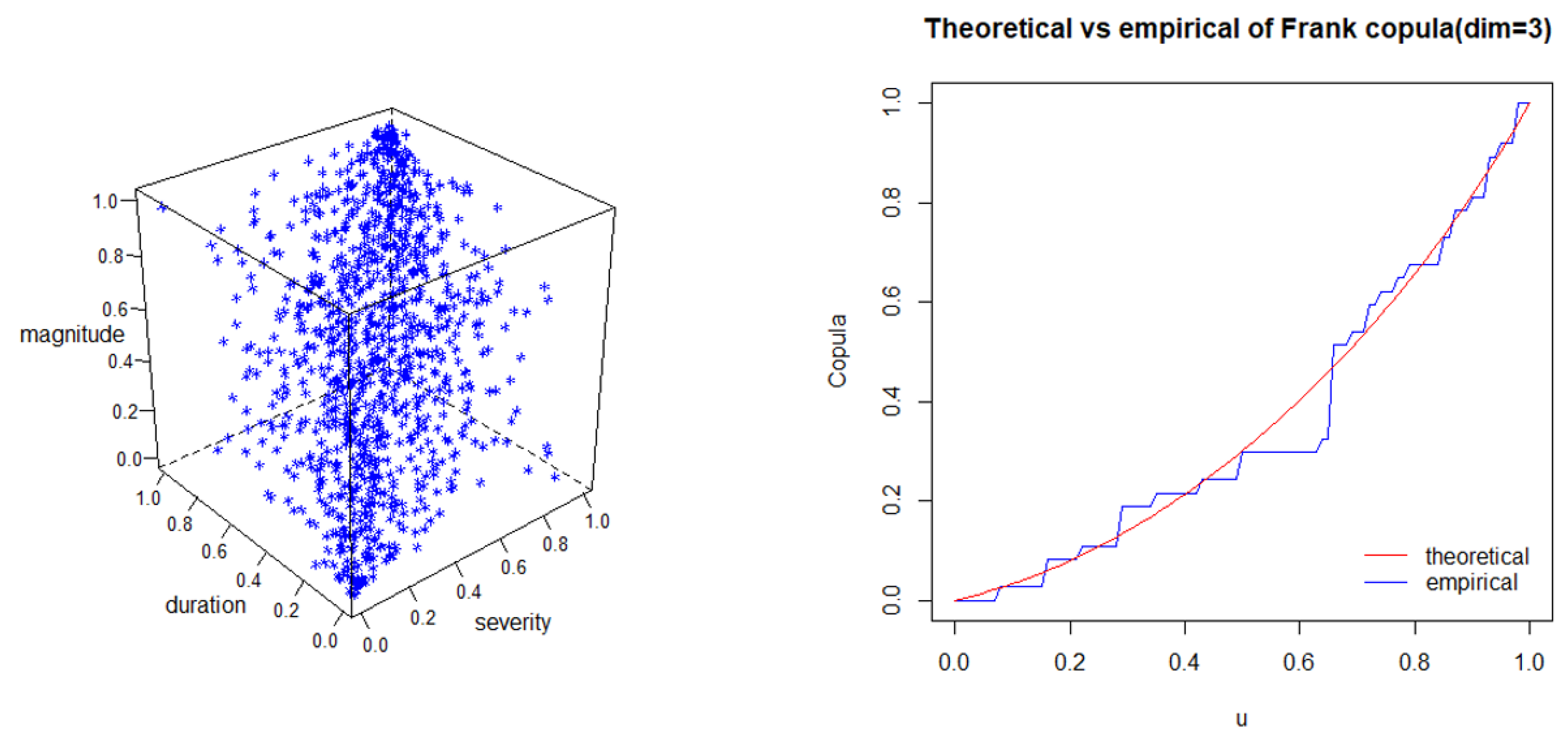
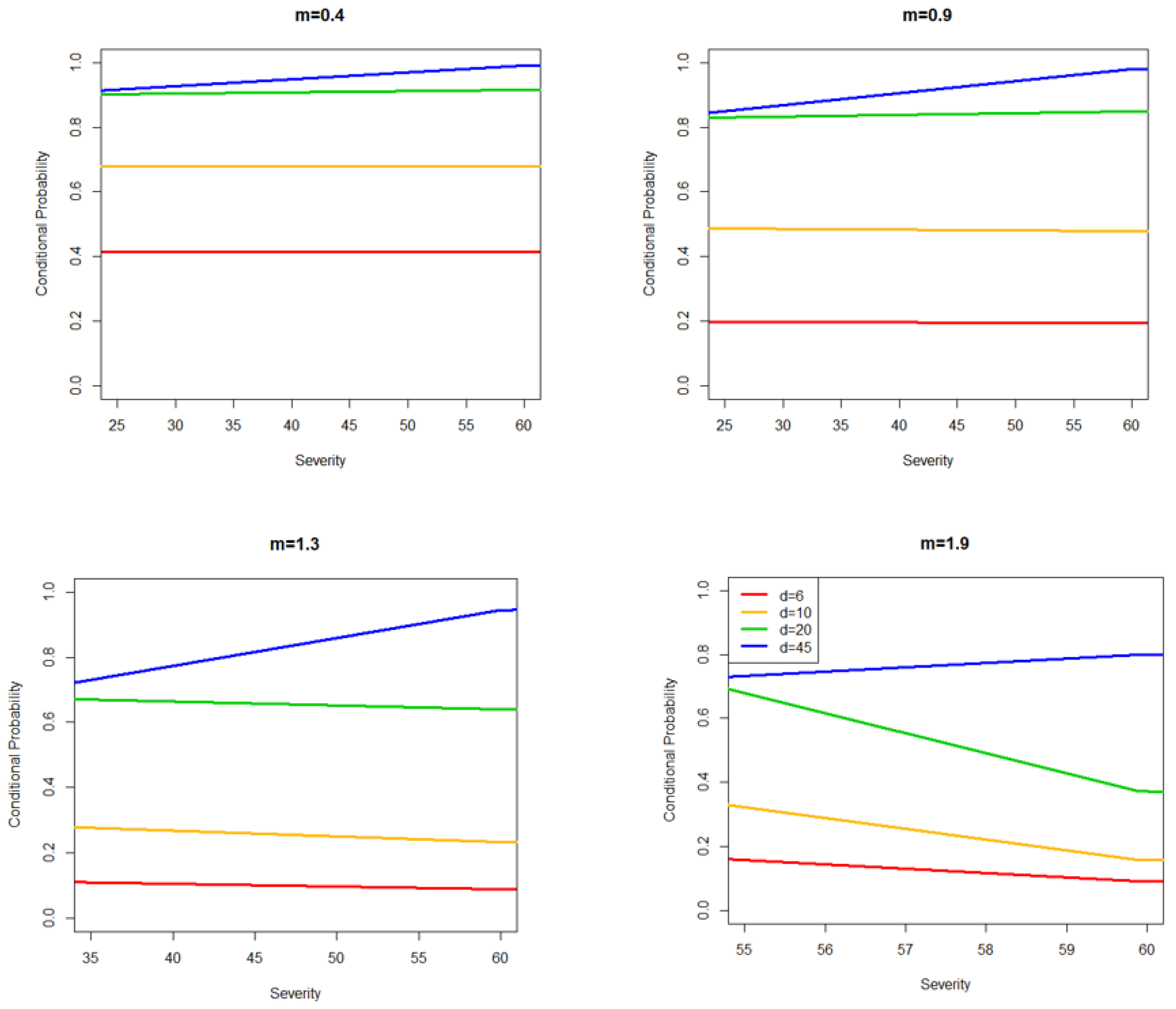
3.8. Conditional Trivariate Return Period and Risk Analysis

For the conditional trivariate return period, the probability of drought severity was estimated in four scenarios. Thresholds include m = 0.4, 0.9, 1.3, and 1.9 and d = 6, 10, 20, and 45, which include the range of values that may occur in the study area. According to Figure 12, by assuming that the drought duration is constant, the conditional probability of the drought severity decreases as the magnitude increases from 0.3 to 0.9.

For example, the conditional probability of S ≤ 50, D ≤ 45 months on M ≥ 0.4, M ≥ 0.9 M ≥ 1.3, M ≥ 1.9 are respectively 0.9 (return period = 10 years), 0.85 (6.6 years), 0.81 (5.26 years), and 0.76 (4.16 years). This means that increasing the hydro-meteorological drought magnitude causes the conditional return period for given severity and duration to decrease.

The trivariate drought risk value can be obtained with $R=1-{\left(1-1/T\right)}^N$. In this equation, T denotes the trivariate conditional return period in the defined scenarios, and N represents the period length (number of years) over which we assess the risk. In this study, we estimated the risk at N = 10 and N = 20 years.

Table 11. Conditional return period and risk in defined scenarios.

	Scenario 1	Scenario 2	Scenario 3	Scenario 4
S	50.00	50.00	50.00	50.00
D	45.00	45.00	45.00	45.00
M	0.30	0.90	1.30	1.90
Return Period conditional	10.00	6.60	5.26	4.16
Risk conditional (N = 10 years)	0.65	0.81	0.88	0.94
Risk conditional (N = 20 years)	0.88	0.96	0.99	1.00

shows the multivariate risk based on the four defined scenarios. According to the results, with increasing magnitude of drought, the return period decreases, and the risk of drought increases.

We divided the risk into five classes: without risk (0–0.2), low (0.2–0.4), medium (0.4–0.6), high (0.6–0.8) and very high (>0.8). At N = 10 years, scenario 1 (S = 50, D = 45, M = 0.3) is in the high risk class and other scenarios are in the very high risk class. But in N = 20 years, all scenarios are in the very high risk class such that scenario 4 will be the final risk limit (R close to 1) in the region.

4. Discussion

The basis of drought risk assessment is having sufficient knowledge of this phenomenon. Therefore, due to the different behavior of drought, it is necessary to describe drought from a multivariate perspective. The aim of this study was to analyze the multivariate risk of hydro-meteorological drought in the Wadi Ouahrane Basin. To obtain SPI^mod and SRI^mod, the cumulated rainfall and runoff values of 1 to 12 months based on the moving time window were averaged; then, marginal distribution functions were fitted. The results showed that the gamma function has the best fit for precipitation and the log normal function has the best fit on the runoff. Shukla and Wood [35] showed that in small watersheds, the runoff variable is often a normal function, and in large watersheds, the gamma function is best. Results of our study are confirmed by Yusof et al. [58], who found log-normal distribution as the best fitting distribution for drought severity.

The basis of the joint of two variables is their correlation structure. The results of cross-correlation between ${\mathrm{SPI}}_W^{\mathrm{mod}}$ and ${\mathrm{SRI}}_W^{\mathrm{mod}}$ for w = 1, 2, …, 12 showed that when the time window increases, the correlation also increases, indicating the importance of last year’s rainfall and runoff status compared to rainfall and runoff on a month-to-month basis to identify long-term droughts.

The results of the study of univariate drought indices and multivariate indices showed that the interpretation of drought based on univariate indices, such as ${\mathrm{SPI}}_1^{\mathrm{mod}}$ or ${\mathrm{SRI}}_1^{\mathrm{mod}}$ is more complex. Because these indicators only check for one month in drought monitoring, they are not able to accurately detect the time of drought. However, the multivariate hydrological and meteorological indicators obtained by copula show the drought status based on the structure of dependence between the precipitation and streamflow of the last 12 months, thus providing acceptable results for drought monitoring. In addition, the results of time series of indices showed that multivariate indices follow a similar trend, with less variability compared to univariate index.

Comparison of the changes in univariate indices (SPI, SRI) and multivariate indices due to hydrological and meteorological drought (JDMI, JDHI) with the hydro-meteorological composite index (JDHMI) showed that all have a relatively similar trend, but sometimes, the behavior of runoff was incompatible and specific. It seems that the most important factor for runoff incompatibility behavior is snowfall in some years. The results of Azhdari et al. [53,59] also confirmed runoff incompatibility in arid and semi-arid regions. It seems that the reason for this incompatibility is the changes in the precipitation regime and the complexity of the mechanism for converting precipitation to runoff in these areas.

According to Azhdari et al. [53], the composite indices reflected the comprehensive moisture status of the catchment well and were not affected by a single element. Presented analysis confirmed the study of Azhdari et al. [53], who found runoff was the main source of inconsistency in the study region.

The results of the correlation coefficient between the studied indices show that the correlation of univariate indices is less than 0.5, but for the multivariate and hybrid indices, the correlation is higher than 0.7. Therefore, the joint of the indicators improves the recognition of the occurrence of multi-timescale hydro-meteorological droughts. This statement is supported by Dehghani et al. [60], who found that joint indicators and copula functions can show relationships between the variables that determine drought that are not visible from classical analysis. In addition, the calculation of the weighted kappa coefficient showed that the degree of agreement between the composite indicators is high. Therefore, it can be concluded that the composite index performs better in drought monitoring and has a good agreement with rainfall and runoff. The results of comparing JDHMI with other univariate and multivariate indices showed that JDHMI can present the possibility of a common hydrological and meteorological deficit situation more accurately and realistically than other indices.

The results of three-variable conditional risk analysis with different scenarios showed that considering different thresholds for variables affecting drought risk has an effective role in drought warning. Ignoring the simultaneous or conditional effects of these variables will have negative consequences on water and soil resources.

In bivariate modeling in hydrology and hydrometeorology, the main advantage of copulas is the modeling of the joint dependency structure without any limitation on the marginal distributions. Therefore, given this important performance, researchers can flexibly select marginal and common probability functions. As a result, the choice of marginal distribution is critical because it strongly affects the copula’s performance in modeling bivariate variables, and any mistake in their selection leads to overestimation or underestimation in risk analysis. On the other hand, selecting the appropriate distribution function from among the candidates is also time consuming. The principle of maximum entropy provides a more objective way to derive probability distribution functions (PDFs) with a minimum bias of finite information, in which the PDF has maximum uncertainty, subject to a set of constraints that can be a good alternative copula method [61]. However, the proposed method is in the early stages of development, so more research is needed to prove its superiority over the copula method.

Finally, it can be concluded that composite indices are more suitable for drought assessment and pre-warning than univariate and multivariate indices, because they show several types of drought simultaneously. Moreover, according to Chen et al. [62], the joint probabilities and return periods of drought give important information for water management and planning. Therefore, due to the variability of climate variables in recent years, the findings of this research will be useful for reducing the effects of drought on natural resources, planning for future water resource development, and changing cultivation patterns in areas with similar conditions.

5. Conclusions

The meteorological and hydrological drought condition in the Wadi Ouahrane Basin, Algeria, was investigated using copulas for multivariate drought characteristics. The study was performed in the Mediterranean region of North Africa, which is characterized by a very dynamic climate, high variability of rainfall and thermal conditions, and high variability of the hydrological regime. In this region, water scarcity is common. Meteorological and hydrological drought were analyzed based on SPI and SRI at different timescales, from 1 to 12 months, and the conditional return period for both types of drought was evaluated by means of the copula function. The analysis showed that gamma and log-normal distribution were the best fitted models describing the monthly series of rainfall and runoff drought indexes. As can be expected, runoff is characterized by a high level of temporal correlation in comparison to rainfall. This can be the result of higher lag of the river on the rainfall deficit. Using the copula parametric function, the two joint deficit indices JDMI and JDHI were combined, and JDHMI was obtained. The composite index JDHMI is able to better reflect the simultaneous hydrological and meteorological behavior well and can present the probability of a common hydrological and meteorological deficit situation more accurately and realistically than univariate and multivariate precipitation-based indicators or runoff alone. Our study showed that JDMI and JDHI gave different results compared to traditional SPI and SRI indices, and they are more sensitive to rainfall structure than SPI or SRI at any one timescale. Finally, based on the composite index JDHMI, it was found that over the analyzed basin, the average severity of hydro-meteorological drought in the study area was 10.19, with a duration of 9 months, and its magnitude was 0.93. The achieved results showed that complex indexes can better reflect drought because they reflect correlations in hydrological and meteorological drought across a range of timescales, and thus can help with preparing regional or national strategies and planning for drought mitigation.

References

1. AghaKouchak, A.; Mirchi, A.; Madani, K.; Di Baldassarre, G.; Nazemi, A.; Alborzi, A.; Anjileli, H.; Azarderakhsh, M.; Chiang, F.; Hassanzadeh, E.; et al. Anthropogenic Drought: Definition, Challenges, and Opportunities. Rev. Geophys. 2021, 59, e2019RG000683. [Google Scholar] [CrossRef]
2. Bissenbayeva, S.; Abuduwaili, J.; Saparova, A.; Ahmed, T. Long-term variations in runoff of the Syr Darya River Basin under climate change and human activities. J. Arid. Land 2021, 13, 56–70. [Google Scholar] [CrossRef]
3. Dhaubanjar, S.; Lutz, A.F.; Gernaat, D.E.; Nepal, S.; Smoolenars, W.; Pradhanaga, S.; Biemans, H.; Shrestha, A.B.; Immerzeel, W.W.; Ludwig, F. A systematic framework for the assessment of sustainable hydropower potential in a river basin—The case of the upper Indus. Sci. Total Environ. 2021, 786, 147142. [Google Scholar] [CrossRef] [PubMed]
4. Tomczyk, P.; Willems, P.; WIatkowski, M. Comparative analysis of changes in hydromorphological conditions upstream and downstream hydropower plants on selected rivers in Poland and Belgium. J. Clean. Prod. 2021, 328, 129524. [Google Scholar] [CrossRef]
5. Liu, Q.; Niu, J.; Sivakumar, B.; Ding, R.; Li, S. Accessing future crop yield and crop water productivity over the Heihe River basin in northwest China under a changing climate. Geosci. Lett. 2021, 8, 2. [Google Scholar] [CrossRef]
6. Brouziyne, Y.; De Girolamo, A.M.; Aboubdillah, A.; Benaabidate, L.; Bouchaou, L.; Chehbouni, A. Modeling alterations in flow regimes under changing climate in a Mediterranean watershed: An analysis of ecologically-relevant hydrological indicators. Ecol. Inform. 2021, 61, 101219. [Google Scholar] [CrossRef]
7. Liu, W.; Bailey, R.T.; Andersen, H.E.; Jeppesen, E.; Nielsen, A.; Peng, K.; Molina-Navarro, E.; Park, S.; Thodsen, H.; Trolle, D. Quantifying the effects of climate change on hydrological regime and stream biota in a groundwater-dominated catchment: A modelling approach combining SWAT-MODFLOW with flow-biota empirical models. Sci. Total Environ. 2020, 745, 140933. [Google Scholar] [CrossRef]
8. Henriksen, H.J.; Jakobsen, A.; Pasten-Zapata, E.; Troldborg, L.; Sonnenborg, T.O. Assessing the impacts of climate change on hydrological regimes and fish EQR in two Danish catchments. J. Hydrol. Reg. Stud. 2021, 34, 100798. [Google Scholar] [CrossRef]
9. Dahri, Z.H.; Ludwig, F.; Moors, E.; Ahmad, S.; Ahmad, B.; Ahmad, S.; Riaz, M.; Kabat, P. Climate change and hydrological regime of the high-altitude Indus basin under extreme climate scenarios. Sci. Total Environ. 2021, 768, 144467. [Google Scholar] [CrossRef]
10. Saifullah, M.; Adnan, M.; Zaman, M.; Wałęga, A.; Liu, S.; Khan, M.I.; Gagnon, A.S.; Muhammad, S. Hydrological Response of the Kunhar River Basin in Pakistan to Climate Change and Anthropogenic Impacts on Runoff Characteristics. Water 2021, 13, 3163. [Google Scholar] [CrossRef]
11. De Fries, R.S.; Foley, J.A.; Asner, G.P. Land-Use Choices: Balancing Human Needs and Ecosystem Function. Front. Ecol. Environ. 2004, 2, 249–257. [Google Scholar] [CrossRef]
12. Wang, F.; Wang, Z.; Yang, H.; Di, D.; Zhao, Y.; Liang, Q.; Hussain, Z. Comprehensive evaluation of hydrological drought and its relationships with meteorological drought in the Yellow River basin, China. J. Hydrol. 2020, 584, 124751. [Google Scholar] [CrossRef]
13. Viola, M.R.; Mello, C.R.; Beskow, S.; Norton, L.D. Impacts of land-use changes on the hydrology of the Grande river basin headwaters, Southeastern Brazil. Water Resour. Manag. 2014, 28, 4537–4550. [Google Scholar] [CrossRef]
14. Lopes, T.R.; Zolin, C.A.; Mingoti, R.; Vendrusculo, L.G.; Terra de Almeida, F.; de Souza, A.P.; de Oliveira, R.F.; Paulino, J.; Uliana, E.M. Hydrological regime, water availability and land use/land cover change impact on the water balance in a large agriculture basin in the Southern Brazilian Amazon. J. S. Am. Earth Sci. 2021, 108, 103224. [Google Scholar] [CrossRef]
15. Zhang, M.; Liu, N.; Harper, R.; Li, Q.; Liu, K.; Wei, X.; Ning, D.; Hou, Y.; Liu, S. A global review on hydrological responses to forest change across multiple spatial scales: Importance of scale, climate, forest type and hydrological regime. J. Hydrol. 2017, 546, 44–59. [Google Scholar] [CrossRef] [Green Version]
16. Dorjsuren, B.; Batsaikhan, N.; Yan, D.; Yadamjav, O.; Qin, T.; Weng, B.; Bi, W.; Demberel, O.; Gombo, O.; Girma, A.; et al. Study on Relationship of Land Cover Changes and Ecohydrological Processes of the Tuul River Basin. Sustainability 2021, 13, 1153. [Google Scholar] [CrossRef]
17. Wojkowski, J.; Młyński, D.; Lepeška, T.; Wałęga, A.; Radecki-Pawlik, A. Link between hydric potential and predictability of maximum flow for selected catchments in Western Carpathians. Sci. Total Environ. 2019, 683, 293–307. [Google Scholar] [CrossRef]
18. Buttafuoco, G.; Caloiero, T.; Ricca, N.; Guagliardi, I. Assessment of drought and its uncertainty in a southern Italy area (Calabria region). Measurement 2018, 113, 205–210. [Google Scholar] [CrossRef]
19. Caloiero, T.; Veltri, S. Drought Assessment in the Sardinia Region (Italy) During 1922–2011 Using the Standardized Precipitation Index. Pure Appl. Geophys. 2019, 176, 925–935. [Google Scholar] [CrossRef]
20. Zhu, U.; Liu, Y.; Wang, W.; Singh, V.P.; Ma, X.; Yu, Z. Three dimensional characterization of meteorological and hydrological droughts and their probabilistic links. J. Hydrol. 2019, 578, 124016. [Google Scholar] [CrossRef]
21. Li, Q.; He, P.; He, Y.; Han, X.; Zeng, T.; Lu, G.; Wang, H. Investigation to the relation between meteorological drought and hydrological drought in the upper Shaying River Basin using wavelet analysis. Atmos. Res. 2020, 234, 104743. [Google Scholar] [CrossRef]
22. Jehanzaib, M.; Yoo, J.; Kwon, H.-H.; Kim, T.-W. Reassessing the frequency and severity of meteorological drought considering non-stationarity and copula-based bivariate probability. J. Hydrol. 2021, 603, 126948. [Google Scholar] [CrossRef]
23. Ding, Y.; Xu, J.; Wanga, X.; Cai, H.; Zhou, Z.; Sun, Y.; Shi, H. Propagation of meteorological to hydrological drought for different climate regions in China. J. Environ. Manage. 2021, 283, 111980. [Google Scholar] [CrossRef] [PubMed]
24. Bevacqua, A.G.; Chaffe, P.L.B.; Chagas, V.B.P.; AghaKouchak, A. Spatial and temporal patterns of propagation from meteorological to hydrological droughts in Brazil. J. Hydrol. 2021, 603, 126902. [Google Scholar] [CrossRef]
25. Zhang, T.; Su, X.; Feng, K. The development of a novel nonstationary meteorological and hydrological drought index using the climatic and anthropogenic indices as covariates. Sci. Total Environ. 2021, 786, 147385. [Google Scholar] [CrossRef]
26. Ho, S.; Tian, L.; Disse, M.; Tuo, Y. A new approach to quantify propagation time from meteorological to hydrological drought. J. Hydrol. 2021, 603, 127056. [Google Scholar] [CrossRef]
27. Gu, L.; Chen, J.; Yin, J.; Xu, C.; Chen, H. Drought hazard transferability from meteorological to hydrological propagation. J. Hydrol. 2020, 585, 124761. [Google Scholar] [CrossRef]
28. Farrokhi, A.; Farzin, S.; Mousavi, S.-H. Meteorological drought analysis in response to climate change conditions, based on combined four-dimensional vine copulas and data mining (VC-DM). J. Hydrol. 2021, 603, 127135. [Google Scholar] [CrossRef]
29. Wang, Y.; Zhang, X.; Peng, P. Spatio-Temporal Changes of Land-Use/Land Cover Change and the Effects on Ecosystem Service Values in Derong County, China, from 1992–2018. Sustainability 2021, 13, 827. [Google Scholar] [CrossRef]
30. Achite, M.; Krakauer, N.Y.; Wałęga, A.; Caloiero, T. Spatial and Temporal Analysis of Dry and Wet Spells in the Wadi Cheliff Basin, Algeria. Atmosphere 2021, 12, 798. [Google Scholar] [CrossRef]
31. Achite, M.; Wałęga, A.; Toubal, A.K.; Mansour, H.; Krakauer, N. Spatiotemporal Characteristics and Trends of Meteorological Droughts in the Wadi Mina Basin, Northwest Algeria. Water 2021, 13, 3103. [Google Scholar] [CrossRef]
32. Fellag, M.; Achite, M.; Walega, A. Spatial-temporal characterization of meteorological drought using the Standardized precipitation index. Case study in Algeria. Acta Sci. Pol. Form. Circumiectus 2021, 20, 19–31. [Google Scholar] [CrossRef]
33. Benzater, B.; Elouissi, A.; Dabanli, I.; Harkat, S.; Hamimed, A. New approach to detect trends in extreme rain categories by the ITA method in northwest Algeria. Hydrol. Sci. J. 2021, 66, 2298–2311. [Google Scholar] [CrossRef]
34. McKee, T.B.; Doesken, N.J.; Kleist, J. The relationship of drought frequency and duration to time scales. In Proceedings of the 8th Conference of Applied Climatology, Anaheim, CA, USA, 17–22 January 1993; pp. 179–184. [Google Scholar]
35. Shukla, S.; Wood, A.W. Use of a standardized runoff index for characterizing hydrologic drought. Geophys. Res. Lett. 2008, 35, 226–236. [Google Scholar] [CrossRef] [Green Version]
36. Kao, S.C.; Govindaraju, R.S. A copula based joint deficit index for droughts. J. Hydrol. 2010, 380, 121–134. [Google Scholar] [CrossRef]
37. Loukas, A.; Vasiliades, L. Probabilistic analysis of drought spatiotemporal characteristics in Thessaly region, Greece. Natl. Hazards Earth Syst. Sci. 2004, 4, 719–731. [Google Scholar] [CrossRef]
38. Xiao, H.; Siddiqua, M.; Braybrook, S.; Nassuth, A. Three grape CBF/DREB1 genes respond to low temperature, drought and abscisic acid. Plant Cell Environ. 2006, 29, 410–1421. [Google Scholar] [CrossRef] [Green Version]
39. Shiau, J.T.; Modarres, R. Copula-based drought severity-duration-frequency analysis in Iran. Met. Apps. 2009, 16, 481–489. [Google Scholar] [CrossRef]
40. Mirabbasi, R.; Anagnostou, E.N.; Fakheri-Fard, A.; Dinpashoh, Y.; Eslamian, S. Analysis of meteorological drought in northwest Iran using the joint deficit index. J. Hydrol. 2013, 492, 35–48. [Google Scholar] [CrossRef]
41. Caloiero, T.; Caroletti, G.N.; Coscarelli, R. IMERG-Based Meteorological Drought Analysis over Italy. Climate 2021, 9, 65. [Google Scholar] [CrossRef]
42. Sklar, A. Fonctions de repartition a n dimensions et leurs marges. Publ. Inst. Stat. Univ. Paris 1959, 8, 229–231. [Google Scholar]
43. Bazrafshan, O.; Zamani, H.; Shekari, M. A copula-based index for drought analysis in arid and semi-arid regions of Iran. Nat. Resour. Model. 2020, 33, e12237. [Google Scholar] [CrossRef]
44. Bazrafshan, O.; Zamani, H.; Shekari, M.; Singh, V.P. Regional risk analysis and derivation of copula-based drought for severity-duration curve in arid and semi-arid regions. Theor. Appl. Climatol. 2020, 141, 889–905. [Google Scholar] [CrossRef]
45. Li, X.; Babovic, V. Multi-site multivariate downscaling of global climate model outputs: An integrated framework combining quantile mapping, stochastic weather generator and Empirical Copula approaches. Clim. Dyn. 2019, 52, 5775–5799. [Google Scholar] [CrossRef]
46. Schefzik, R.; Thorarinsdottir, T.L.; Gneiting, T. Uncertainty quantification in complex simulation models using Ensemble Copula coupling. Stat. Sci. 2013, 28, 616–640. [Google Scholar] [CrossRef]
47. Kao, S.C.; Govindaraju, R.S. Trivariate statistical analysis of extreme rainfall events via the Plackett family of copulas. Water Resour. Res. 2008, 44, 102–115. [Google Scholar] [CrossRef]
48. Durrleman, V.; Nikeghbali, A.; Roncalli, T. Which Copula is the Right One? Available online: https://ssrn.com/abstract=10325 (accessed on 9 January 2022).
49. Akaike, H. Information Theory and an Extension of the Maximum Likelihood Principle. In Proceedings of the 2nd International Symposium on Information Theory, Tsahkadsor, Armenia, 2–8 September 1971; Petrov, B.N., Csaki, F., Eds.; Akademiai Kiado: Budapest, Hungary, 1973; pp. 267–281. [Google Scholar]
50. Schweizer, B.; Wolff, E.F. On Nonparametric Measures of Dependence for Random Variables. Ann. Stat. 1981, 9, 879–885. [Google Scholar] [CrossRef]
51. Burnham, K.P.; Anderson, D.R. Model Selection and Multimodel Inference: A Practical Information-Theoretical Approach, 2nd ed.; Springer: New York, NY, USA, 2002. [Google Scholar]
52. Azhdari, Z.; Bazrafshan, O.; Shekari, M. Three-dimensional risk analysis of hydro-meteorological drought using multivariate nonlinear index. Theor. Appl. Climatol. 2020, 142, 1311–1327. [Google Scholar] [CrossRef]
53. Azhdari, Z.; Bazrafshan, O.; Zamani, H.; Shekari, M.; Singh, V.P. Hydro-meteorological drought risk assessment using linear and nonlinear multivariate methods. Phys. Chem. Earth 2021, 123, 103046. [Google Scholar] [CrossRef]
54. Hofert, M.; Mächler, M. Nested Archimedean copulas meet R: The nacopula package. J. Stat. Softw. 2011, 39, 1–20. [Google Scholar] [CrossRef] [Green Version]
55. Kao, S.C.; Govindaraju, R.S. Reply to comment by T. P. Hutchinson on “Trivariate statistical analysis of extreme rainfall events via the Plackett family of copulas”. Water Resour. Res. 2010, 46, W04802. [Google Scholar] [CrossRef]
56. Azam, M.; Maeng, S.J.; Kim, H.S.; Murtazaev, A. Copula-Based Stochastic Simulation for Regional Drought Risk Assessment in South Korea. Water 2018, 10, 359. [Google Scholar] [CrossRef] [Green Version]
57. Fisher, N.I.; Switzer, P. Chi-Plots for Assessing Dependence. Biometrika 1985, 72, 253–265. [Google Scholar] [CrossRef]
58. Yusof, F.; Hui-Mean, F.; Suhaila, J.; Yusof, Z. Characterisation of Drought Properties with Bivariate Copula Analysis. Water Resour. Manag. 2013, 27, 4183–4207. [Google Scholar] [CrossRef]
59. Liu, S.; Huang, S.; Xie, Y.; Wang, H.; Huang, Q.; Leng, G.; Li, P.; Wang, L. Spatial-temporal changes in vegetation cover in a typical semi-humid and semi-arid region in China: Changing patterns, causes and implications. Ecol. Indic. 2019, 98, 462–475. [Google Scholar] [CrossRef]
60. Dehghani, M.; Saghafian, B.; Zargar, M. Probabilistic hydrological drought index forecasting based on meteorological drought index using Archimedean copulas. Hydrol. Res. 2019, 50, 1230–1250. [Google Scholar] [CrossRef]
61. Singh, V.P.; Zhang, L. Copula–entropy theory for multivariate stochastic modeling in water engineering. Geosci. Lett. 2018, 5, 6. [Google Scholar] [CrossRef]
62. Chen, L.; Singh, V.P.; Asce, F.; Guo, S.; Mishra, A.K.; Guo, J. Drought Analysis Using Copulas. J. Hydrol. Eng. 2013, 18, 797–808. [Google Scholar] [CrossRef]
Figure 1. Location, topographic characteristics, and pluviometric and hydrometric network of the study area.
Water 14 00653 g001
Figure 2. Details of LULC classes over the catchment.
Water 14 00653 g002
Figure 3. The distribution function of Kc in different values of C U 1 ,   U 2 ,   ,   U 12 joints for the rainfall (a) and runoff (b) of the study area.
Water 14 00653 g003
Figure 4. Flowchart of methodology.
Water 14 00653 g004
Figure 5. Comparison of univariate (SPI, SRI) and multivariate (JDMI, JDHI) drought indices in October 1982.
Water 14 00653 g005
Figure 6. Time series of univariate (SPI-12, SRI-12) (a) and multivariate (JDHI, JDMI) (b) with composite index (JDHMI).
Water 14 00653 g006
Figure 7. Time series of cumulative of univariate (SPI-12, SRI-12) (a) and composite (JDHMI) and multivariate (JDHI, JDMI) indices (b) in the study area.
Water 14 00653 g007
Figure 8. Kendall plot (top) and chi-plot (down) of S-D-M.
Water 14 00653 g008
Figure 9. Graph of goodness of fit test for the marginal distribution functions to drought characteristics.
Water 14 00653 g009
Figure 10. CDF and PDF of goodness of fit test for S-D, S-M, and D-M.
Water 14 00653 g010
Figure 11. Goodness of fit test of t-copula function on S-D-M.
Water 14 00653 g011
Figure 12. Conditional trivariate return period (years).
Water 14 00653 g012