Incorporating the Filling–Spilling Feature of Depressions into Hydrologic Modeling

Abstract

Surface depressions are one of the important impact factors of hydrologic processes and catchment responses. However, in many hydrologic models, the influence of depressions is often simulated in a lumped manner, which results in the insufficient characterization of the filling–spilling–merging–splitting dynamics of depressions and the threshold behavior of the overland flow. The objective of the research reported in this paper is to improve the simulation of depression-influenced hydrologic processes by capturing the threshold control of depressions. To achieve this objective, a Depression-oriented Soil and Water Assessment Tool (SWAT-D) is developed. Specifically, the intrinsic changing patterns of contributing area and depression storage are first determined and further incorporated into the SWAT to simulate the filling–spilling of depressions and depression-influenced overland flow dynamics. The SWAT-D was applied to a depression-dominated watershed in the Prairie Pothole Region to evaluate its performance and capability. The simulated and observed hydrographs at the watershed outlet showed good agreement, with only a 7% deviation between the simulated and observed volumes of discharges in 2004. The NSE values for the simulated monthly average discharges during calibration and validation periods were 0.78 and 0.71, respectively, indicating the ability of the SWAT-D in reproducing the depression-influenced catchment responses. In addition, the SWAT-D was compared with other depression-oriented modeling techniques (i.e., the lumped depression approach and probability distribution models), and the comparisons emphasized the improvement of the SWAT-D and the importance of the research reported in this paper.

1. Introduction

Hydrologic models have become an effective tool to explore the spatial and temporal variations of hydrologic processes, evaluate water quantity and quality, as well as provide valuable information for water resources management and planning [1,2,3,4]. However, it was found that traditional hydrologic models, where surface depressions are often removed to create a well-connected drainage system, tend to overestimate streamflow [5,6,7] and may not reproduce the spatial distribution of water yields [7] for depression-dominated watersheds. Therefore, incorporating the influences of depressions into hydrologic modeling is of significance for understanding depression-oriented hydrologic processes and estimating water resources of depression-dominated areas.

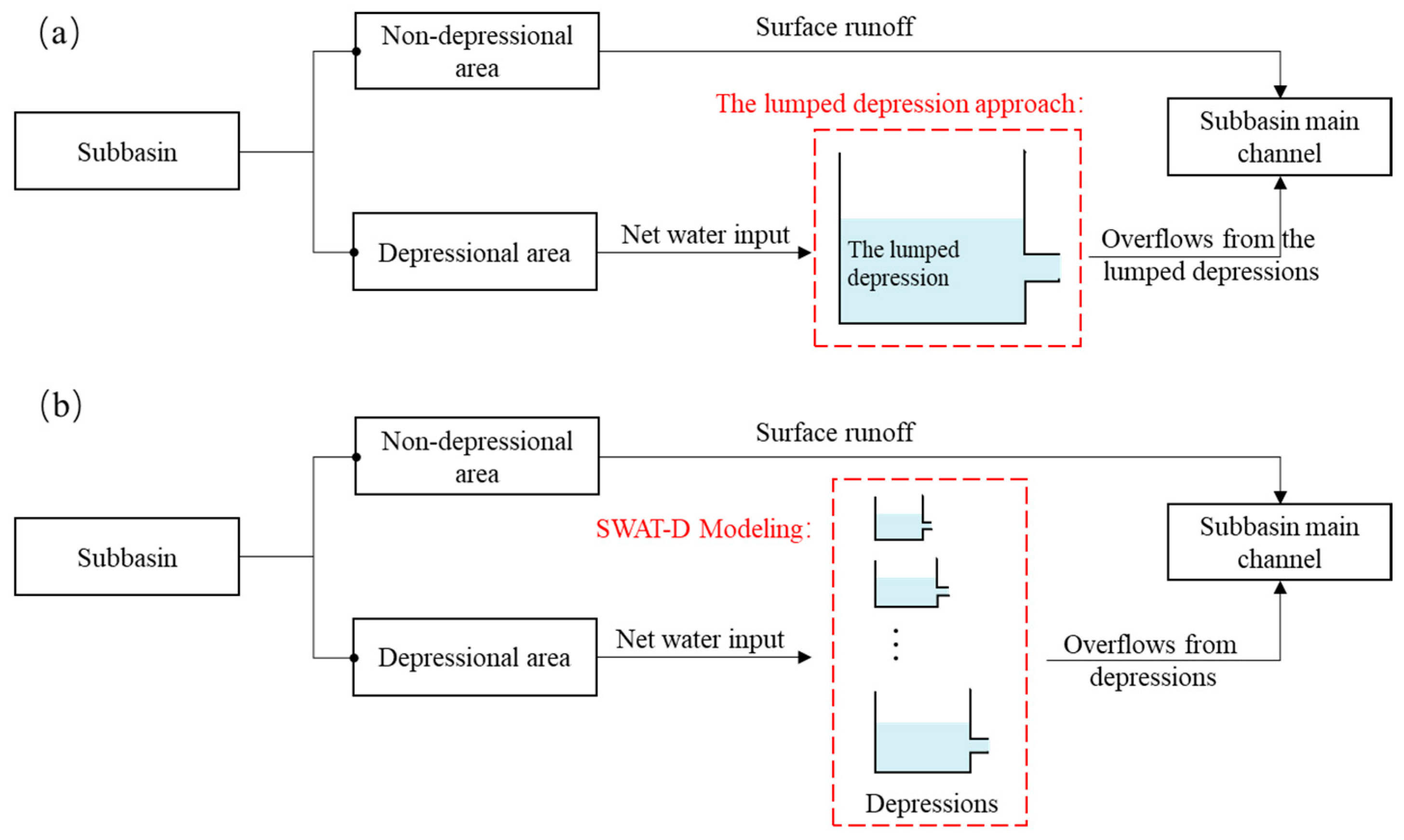
Recently, different models/methods were proposed to simulate the influences of depressions on catchment responses [8,9,10,11,12,13]. For example, the Soil and Water Assessment Tool (SWAT), which is a physically-based watershed-scale model, provides three functions (i.e., Pond, Wetland, and Pothole functions) to deal with the hydrologic impacts of depressions. In the SWAT model, a watershed is divided into a number of subbasins, each of which is further delineated into many hydrologic response units (HRUs) based on the combination of land use, soil type, and slope of the subbasin. By using the Pond/Wetland/Pothole functions, all depressions in a subbasin are aggregated as a lumped depression, and part of the subbasin area (i.e., depressional area) contributes surface runoff to the lumped depression. The non-depressional area of the subbasin contributes surface runoff to the subbasin main channel directly, and the lumped depression overflows to the subbasin main channel when depression storage exceeds its threshold.

The afore-mentioned lumped depression approach can provide reasonable results on outlet discharges after model calibration. However, the real influence of depressions cannot be revealed by the lumped depression approach due to a lack of characterizing the filling–spilling–merging–splitting of depressions [14,15]. To represent the filling–spilling dynamics of overland flow, the hydro-topographic characteristics of depressions were analyzed and implemented to improve depression-dominated hydrologic modeling [14,15,16,17,18,19,20]. For example, Wang et al. [15] developed an event-based, depression-oriented hydrologic model, in which a depression-dominated subbasin was divided into a non-depressional area and a depressional area. For the depressional area, all depressions were lumped together, and Wang et al. [15] summarized the relationship between depression storage and ponding areas of all depressions and determined the hierarchical thresholds to control the gradual water release of the lumped depression. Grimm and Chu [16] analyzed the relationship between depression storage and outflow from the depressional area of a subbasin, which was further employed to improve the lumped depression approach. Zeng and Chu [19,20] identified the intrinsic changing patterns of depression storage and contributing area of a depression-dominated subbasin by tracking the filling–spilling processes of depressions. The determined intrinsic changing patterns were further utilized to simulate the variable contributing area, depression storage, and surface runoff for depression-dominated watersheds. Incorporating the relationships of hydro-topographic properties of depressions to mimic the gradual water release from the depressional area did improve hydrologic modeling for depression-dominated regions, while, at this stage, such modeling methods primarily focused on simulating the filling–spilling of depressions and the threshold-controlled overland flow during a rainfall/snowmelt event.

To mimic the filling–spilling features of depressions, as well as water depletion in depressions under natural conditions, some continuous hydrologic models were developed/proposed. For example, Evenson et al. [21] developed a modified SWAT model, which simulates the water balance of each isolated depression/wetland and the related depression-influenced catchment responses. However, for depression-dominated watersheds, simulating the filling–spilling of individual depressions increases the challenges in input data preparation and model calibration and validation processes for long time periods. To promote long-term modeling for depression-dominated watersheds, Mekonnen et al. [5] and Zeng et al. [22] implemented probability distribution functions of depression storages to simulate the contributing area, depression storage, and surface runoff during rainfall/snowmelt events. However, it was found that the contributing areas estimated by such statistic models may be different from the real ones.

The objective of the research reported in this paper is to improve the simulation of hydrologic processes in depression-dominated watersheds over long time periods. To achieve this objective, the intrinsic hydro-topographic properties of depressions are analyzed, based on which a depression-oriented SWAT (SWAT-D) model is developed to simulate the threshold-controlled, filling–spilling overland flow dynamics during wet periods and water depletion in depressions during dry periods. The SWAT-D model is tested by applying to a depression-dominated watershed in the Prairie Pothole Region, and the simulated discharges at the watershed outlet are compared with the observed ones to demonstrate the abilities of the SWAT-D model in mimicking the depression-dominated hydrologic processes. The SWAT-D is also compared with other depression-oriented modeling techniques (i.e., the lumped depression approach and the probability distribution models) to indicate its improvement and the importance of the research reported in this paper.

2. Materials and Methods

This paper focuses on improved hydrologic modeling for depression-dominated areas over long time periods. To do so, the specific tasks are: (1) delineation of surface depressions and determination of hydro-topographic characteristics, (2) development of a SWAT-D model, which tracks the filling–spilling and water depletion in depressions under natural conditions and mimics the threshold-controlled overland flow dynamics, and (3) evaluation of the performance and improvement of SWAT-D.

2.1. Hydro-Topographic Characteristics of Depressions

Surface depressions have different sizes, shapes, contributing areas, as well as relationships with their surrounding depressions. To account for the hydro-topographic characteristics of depressions, an ArcGIS-based surface delineation algorithm, HUD-DC [23], was used to identify depressions, channel segments, and their contributing areas. The original DEM, depressionless DEM, and the flow directions of a depression-dominated watershed are the input data of the surface delineation processes, based on which the HUD-DC algorithm identifies all depressions and their thresholds as well as all channel segments and channel ending points. Note that each identified depression contains all depressions that have the potential to merge during rainfall/snowmelt events. By setting depression thresholds and channel ending points as pour points, the HUD-DC employs the watershed function of ArcGIS to identify the contributing areas of depressions and channel segments. 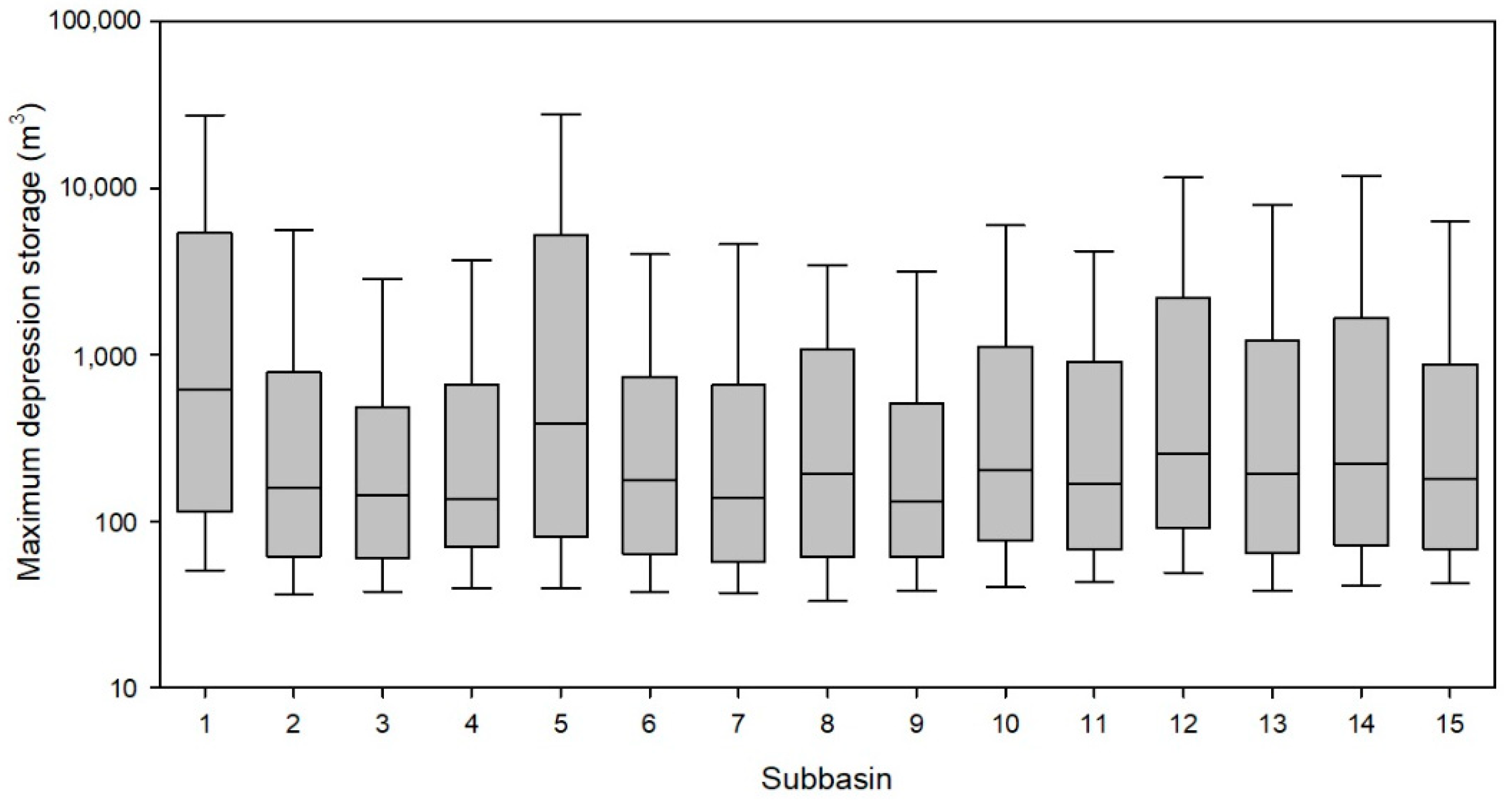Specifically, a depression together with its contributing area is termed as a puddle-based unit (PBU) [24], and a channel segment together with its contributing area is defined as a channel-based unit (CBU) [25]. Finally, the topographic parameters such as maximum depression storage (MDS) of all depressions as well as surface areas of PBUs and CBUs are calculated in the HUD-DC.

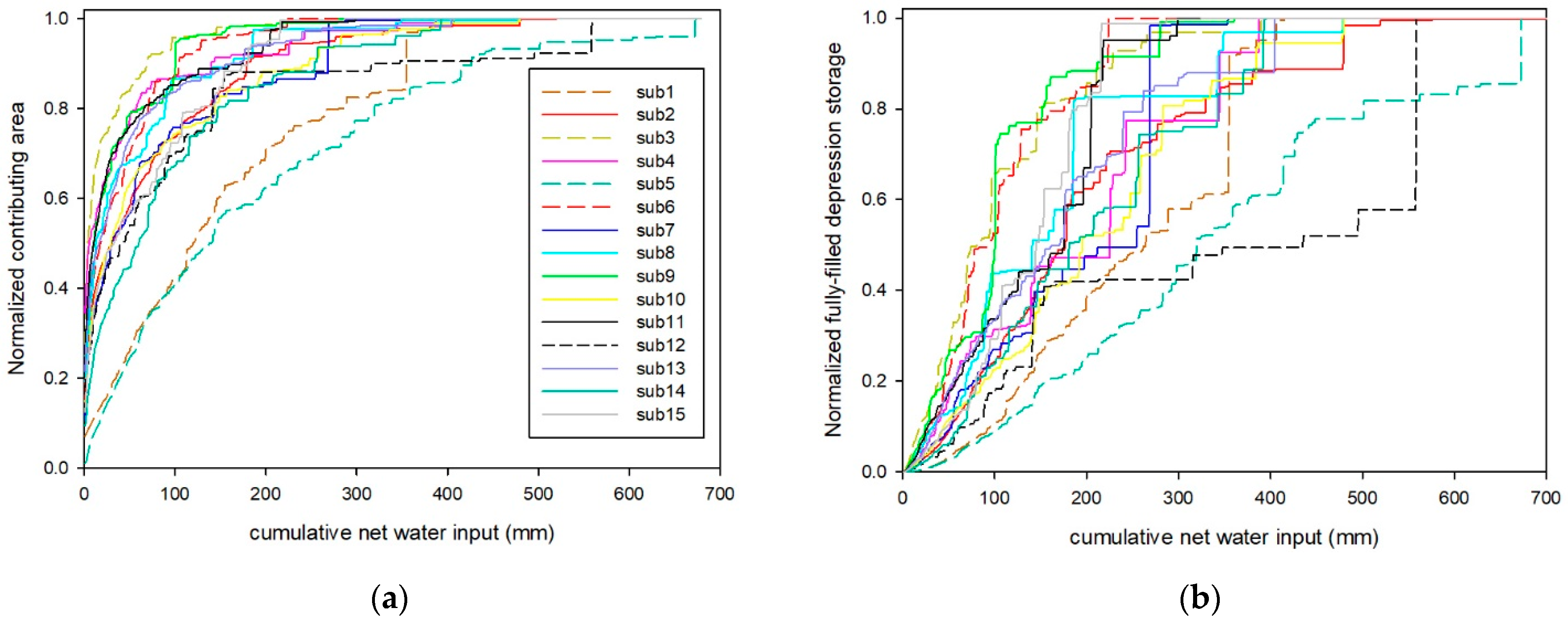
After the surface topography is characterized, the intrinsic influence of depressions on hydrologic connectivity is analyzed by using the method proposed by Zeng and Chu [19]. Specifically, a filling procedure is implemented to determine the relationship between water input and filling–spilling conditions of depressions. For a depression-dominated subbasin, a constant depth of net water input is uniformly applied to fill depressions, and the application of net water input continues until all depressions are fully filled. After each application of the net water input, the filling–spilling condition of each depression is analyzed, and the subbasin-contributing area, which consists of the areas of CBUs and PBUs with fully-filled depressions, is calculated. In addition, the cumulative depression storage of the fully-filled depressions is also computed after each application of net water input. When the fully-filled depression storage reaches the total depression storage of the subbasin (i.e., all depressions are fully filled), the intrinsic changing patterns of fully-filled depression storage and subbasin-contributing area (versus cumulative net water input) are obtained. 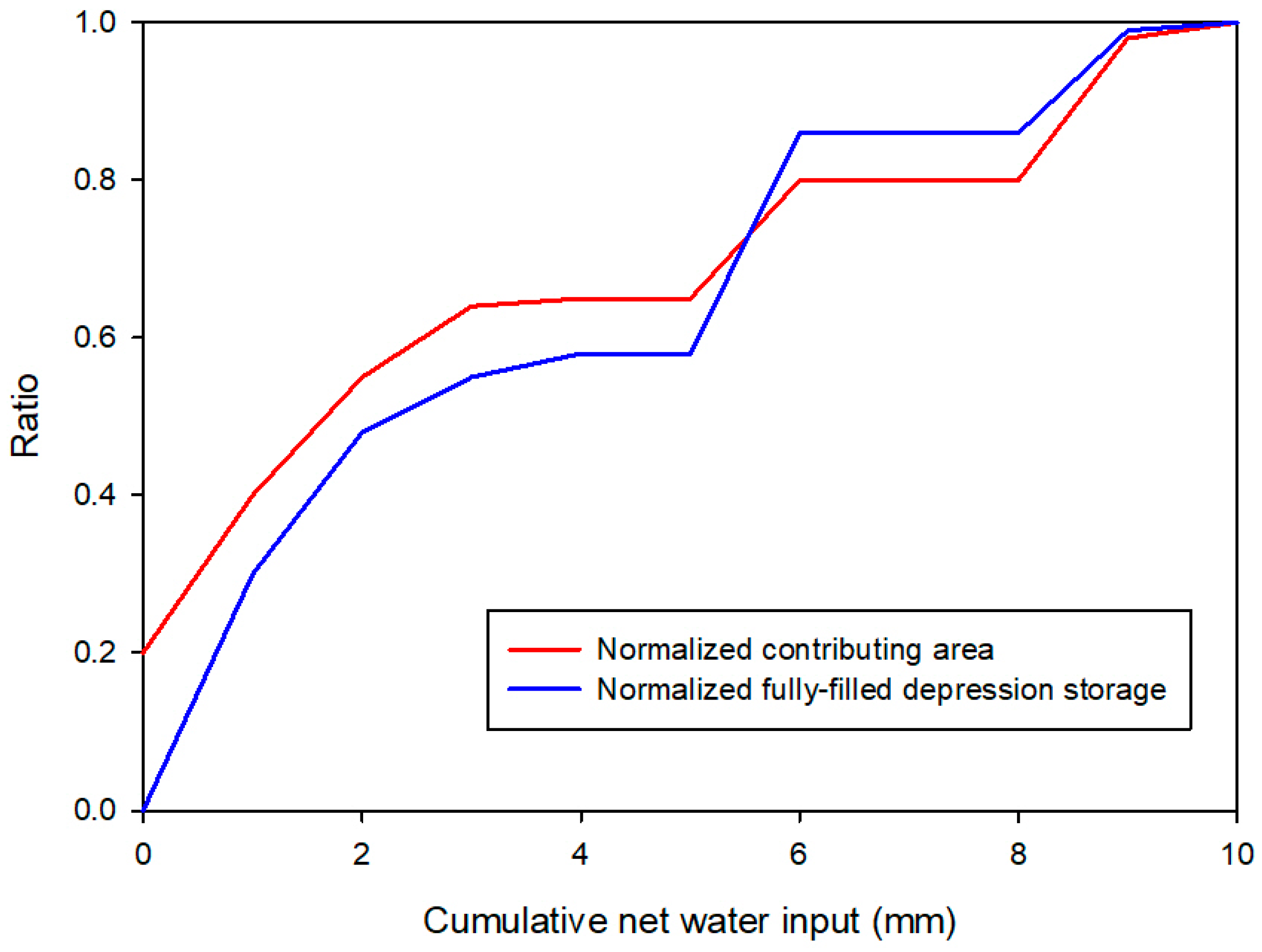Figure 1 shows an example of intrinsic changing patterns of the normalized contributing area and fully-filled depression storage. At the beginning of the application of net water input, the normalized contributing area is greater than zero, which represents the non-depressional area. As the application of net water input continues, the normalized contributing area and fully-filled depression storage increase, and the increase rates depend on the surface topographic characteristics (e.g., surface area and maximum depression storage of depressions). The stepwise patterns of both curves stem from the existence of depressions with larger maximum depression storage values that take a longer time to be fully filled. Such intrinsic changing patterns are further used to determine subbasin-contributing area, depression storage, and surface runoff under natural rainfall conditions; meanwhile, the cumulative net water input is also derived when the subbasin-contributing area or depression storage is known.

2.2. SWAT-D Model

In SWAT, three functions (i.e., Pond, Wetland, Pothole), which utilize the lumped depression approach, are implemented to simulate the hydrologic impacts of depressions. To account for the filling–spilling of all depressions and the depression-oriented hydrologic processes, the SWAT-D is developed in the research reported in this paper. The overall modeling framework of SWAT-D and the modeling method of the threshold-controlled overland flow dynamics are detailed in the following subsections.

2.2.1. Overall Modeling Framework

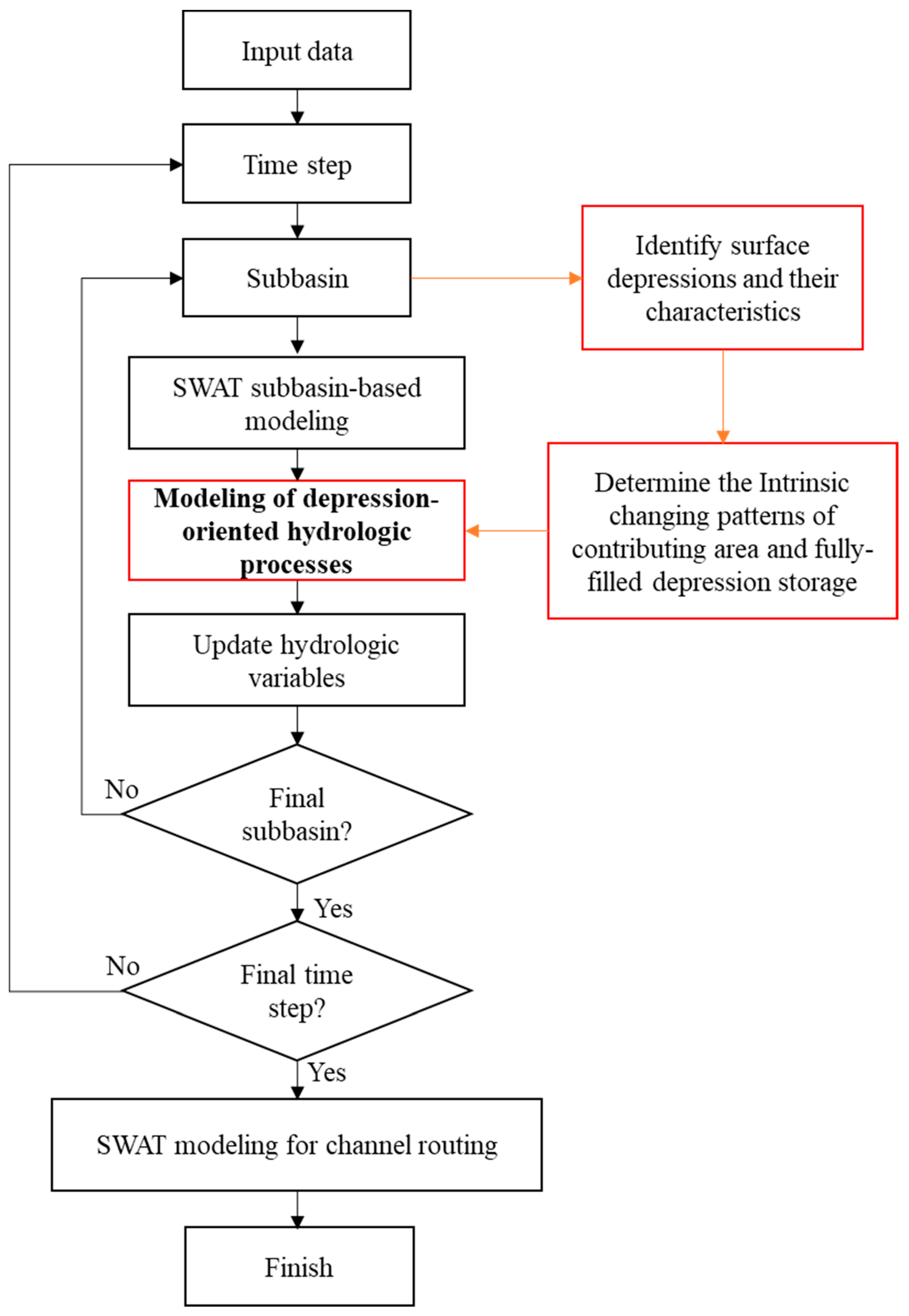
Following the modeling structure of SWAT, SWAT-D is also a semi-distributed hydrologic model, in which a watershed is delineated into a number of subbasins, and SWAT-D implements a time loop and a subbasin loop to simulate the depression-dominated hydrologic processes over long time periods (Figure 2). For each subbasin, the SWAT modeling is first performed to simulate the land phase hydrologic processes such as rainfall excess for filling depressions and generating surface runoff, subsurface flow, and evapotranspiration. Then, the determined intrinsic changing patterns of depression storage and contributing area of the subbasin are incorporated to simulate the impacts of depressions, which is a unique component in SWAT-D as detailed in the following subsection. The water yields of the subbasin are further delivered to the subbasin main channel, which is routed to the watershed outlet throughout the entire channel network.

2.2.2. Modeling of Depression-Oriented Hydrologic Processes

Following Zeng and Chu [19], the intrinsic changing patterns of depression storage and contributing area of a depression-dominated subbasin are determined, which can be further used to simulate the formation of subbasin-contributing area and generation of surface runoff during a rainfall/snowmelt event. Different from the event model proposed by Zeng and Chu [19], SWAT-D is a continuous model in which more impact factors, such as water losses from depressions, are simulated. Therefore, SWAT-D tracks not only the filling–spilling overland flow dynamics during wet time periods but also water depletion in depressions during dry time periods. 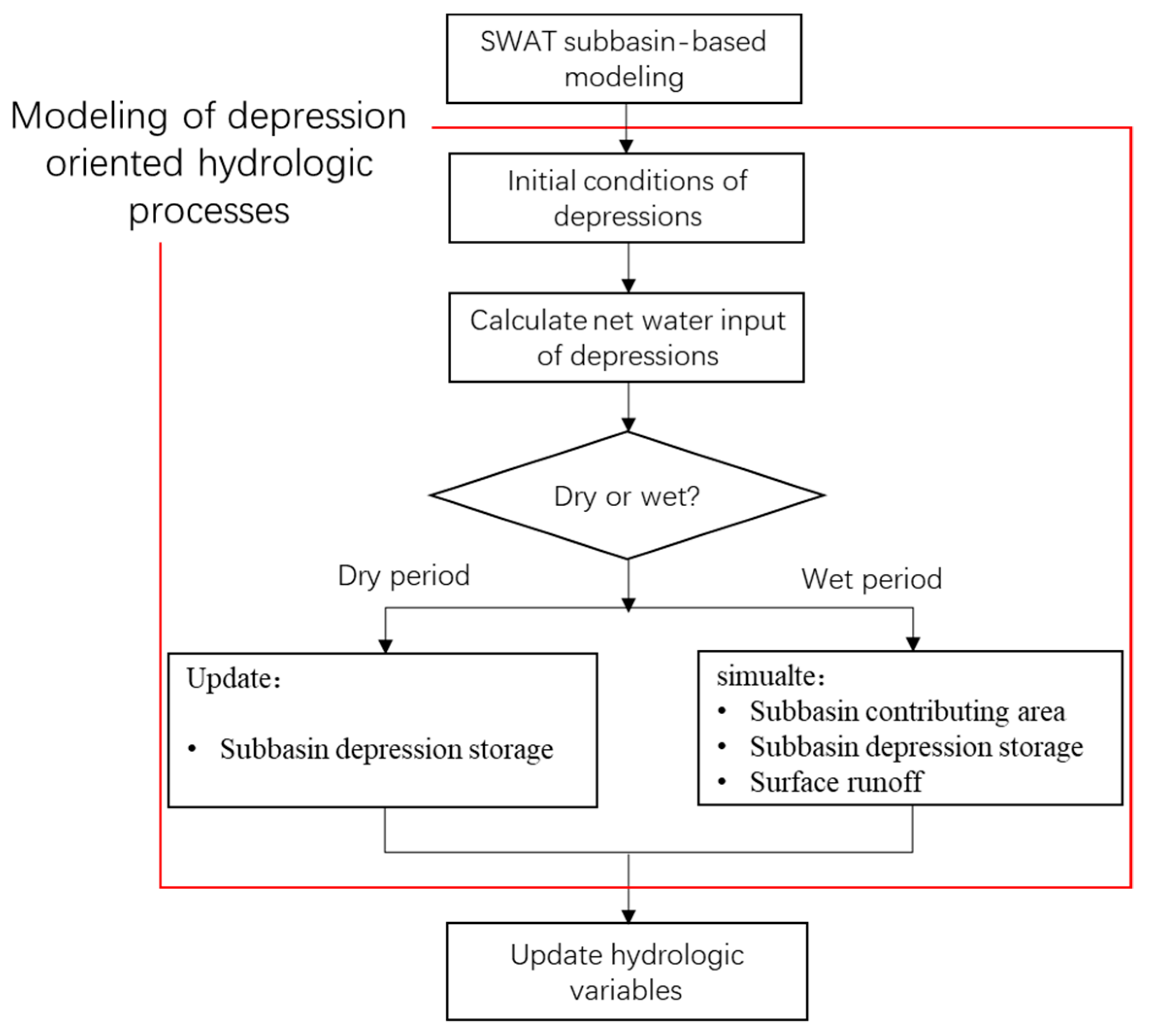Figure 3 shows the modeling framework of the SWAT-D in simulating the depression-oriented hydrologic processes.

In the modeling procedure of a subbasin, the initial conditions at a time step such as initial depression storage of the subbasin are determined first, followed by the calculation of the net water input of depressions of this time step:

$$I_k=P_e{}_k-E_k-S_k$$

(1)

where $I_k$ is net water input of depressions at time step $k$ (m); $P_e{}_k$ is rainfall excess for filling depressions and generating surface runoff at time step $k$ (m); $E_k$ is evaporation from depressions at time step $k$ (m); and $S_k$ is seepage from depressions at time step $k$ (m). Note that $P_e{}_k$, $E_k$, and $S_k$ are considered to be the same for all depressions in a subbasin so that depressions within the same subbasin have an equal depth of net water input $I_k$.

With a positive net water input, the depth of cumulative net water input of depressions is calculated, and surface runoff generated from the subbasin is further simulated based on the intrinsic changing patterns of depression storage and contributing area. That is, the cumulative net water input is compared with the aforementioned intrinsic changing patterns of this subbasin to determine the subbasin-contributing area and depression storage of the contributing area (i.e., fully-filled depression storage) at this time step. Then, surface runoff is generated from the subbasin-contributing area, which is equal to the difference between the amount of net water input and the available depression storage of the subbasin-contributing area:

$$R_k=I_k·C{A}_k-\left(D{S}_k^{CA}-DS{0}_k^{CA}\right)$$

(2)

where $R_k$ is the surface runoff generated from the subbasin at time step $k$ (m³); $C{A}_k$ is the subbasin-contributing area at time step $k$ (m²); $DS{0}_k^{CA}$ and $D{S}_k^{CA}$ are the depression storage of the subbasin-contributing area at the beginning and end of time step $k$ (m³). When the subbasin-contributing area reaches the entire subbasin area, surface runoff generated from the subbasin can be calculated by:

$$R_k=I_k·A-\left(TDS-D{S}_{k-1}\right)$$

(3)

where $A$ is the subbasin area (m²); $TDS$ is the total depression storage of the subbasin (m³); $D{S}_{k-1}$ is the depression storage of the subbasin at time step $k$−1 (m³). The volume of net water input after deducting the generated surface runoff becomes depression storage of the subbasin, and thus, the total depression storage of the subbasin at this time step can be calculated by:

$$D{S}_k=D{S}_{k-1}+\left(A·I_k-R_k\right)$$

(4)

where $D{S}_k$ is the depression storage of the subbasin at time step $k$ (m³).

For a dry time step (i.e., a negative net water input), no surface runoff is generated, and water level in depressions decreases. Then, the subbasin depression storage is updated in the SWAT-D by:

$$D{S}_k=Max\left(D{S}_{k-1}+A·I_k,0\right)$$

(5)

In SWAT-D modeling, the seepage from depressions enters the soil profile, which may flow to the subbasin main channel as lateral flow or recharge the groundwater zone. The water yields of the subbasin (including overland flow, lateral flow, and baseflow) reaching the subbasin main channel are further routed to the watershed outlet throughout the entire channel network.

2.3. Model Application and Evaluation

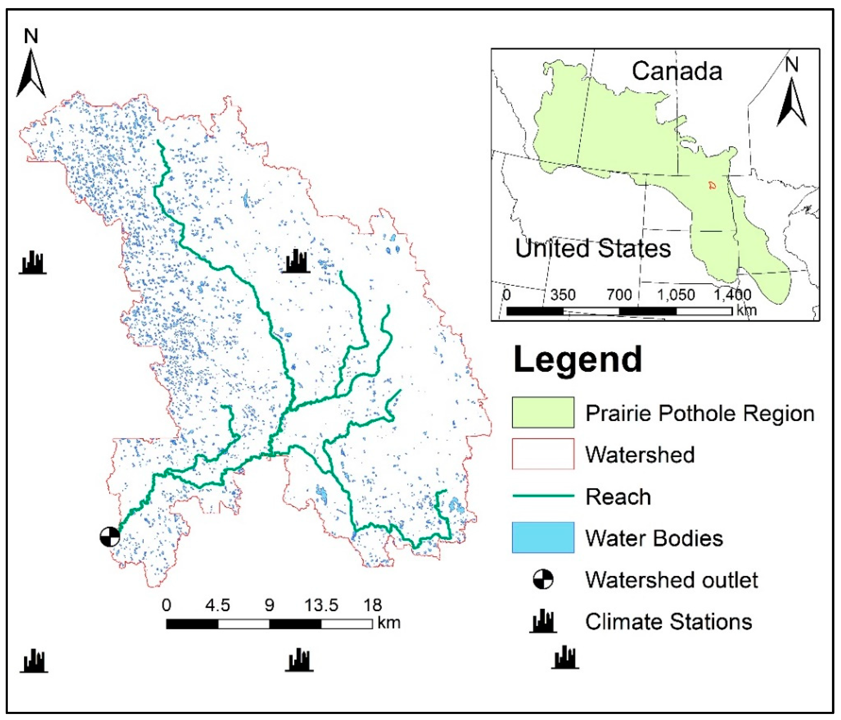
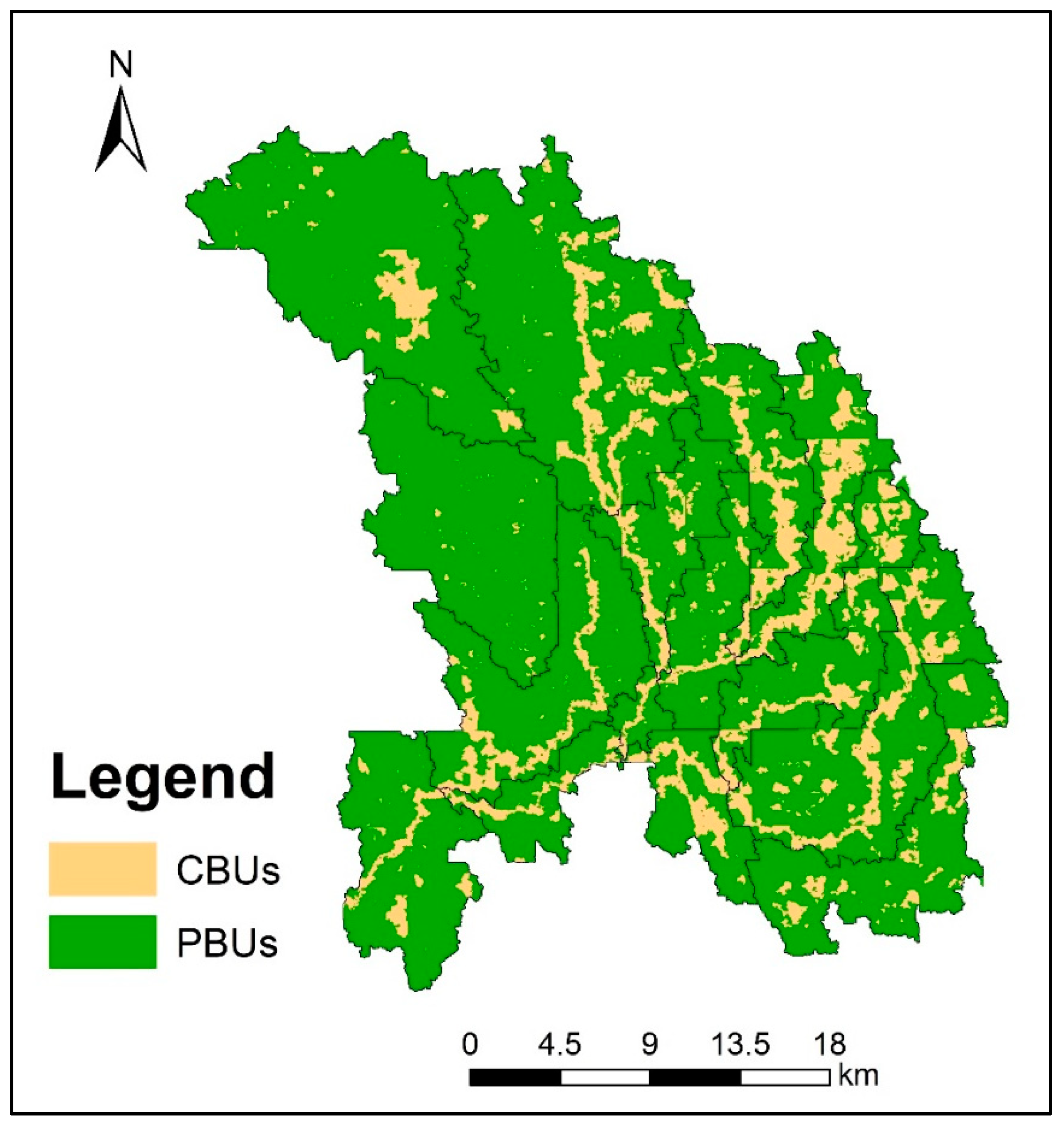
To test the SWAT-D model, a depression-dominated watershed located in the Prairie Pothole Region (PPR) was selected (Figure 4). The watershed outlet is located at the USGS gaging station #05056200 at Edmore Coulee near Edmore, North Dakota (latitude: 48°20′12″ N, longitude: 98°39′36″ W), and its drainage area is about 943 km². Figure 4 shows the spatial distribution of water bodies within the watershed, and the open water and wetlands cover about 13% of the watershed area according to the National Land Cover Database (NLCD 2011).

The input data of SWAT-D consist of DEM, land use, soil type, and meteorological data. In the research reported in this paper, a 10-m DEM, downloaded from the USGS National Map (Available online: https://viewer.nationalmap.gov/basic/, accessed on 9 August 2021), was used for the delineation of the watershed and identification of surface depressions. The land use and soil type data, which were downloaded from the National Land Cover Database (NLCD 2011) (Available online: https://www.mrlc.gov/data/nlcd-2011-land-cover-conus-0, accessed on 9 August 2021) and the State Soil Geographic (STATSGO2) (Available online: https://web-soilsurvey.nrcs.usda.gov/app/WebSoilSurvey.aspx, accessed on 9 August 2021) dataset, respectively, were used to calculate the curve numbers under the average antecedent moisture condition. The meteorological data required by SWAT-D modeling included precipitation, maximum and minimum temperature, solar radiation, relative humidity, and wind speed, which were obtained from the Climate Forecast System Reanalysis (CFSR) (Available online: Global Weather Data for SWAT (tamu.edu), accessed on 7 August 2021). Figure 4 shows the geographic locations of the related climate stations.

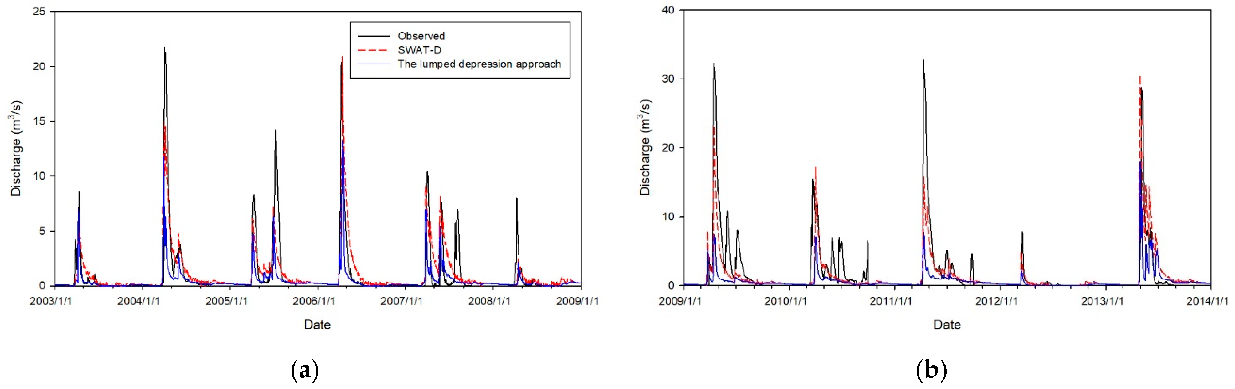
The SWAT-D model was calibrated and validated by using the measured discharges at the watershed outlet, which were downloaded from the USGS National Water Information System (https://maps.waterdata.usgs.gov/mapper/index.html, accessed on 7 August 2021). The calibration and validation periods were 2003–2008 and 2009–2013, respectively. In addition, to set the initial conditions of the model, a 3-year warm-up period from 2000 to 2002 was utilized. To quantitively evaluate the performance of the SWAT-D model, two statistic parameters, Nash–Sutcliffe efficiency (NSE) coefficient [26] and percent bias (PBIAS) [27], were used, and their mathematical expressions are:

$$\mathrm{NSE}=1-\frac{{{\displaystyle \sum }}_{i=1}^n{\left(Q^{obs}{}_i-Q^{sim}{}_i\right)}^2}{{{\displaystyle \sum }}_{i=1}^n{\left(Q^{obs}{}_i-{\overline{Q}}^{obs}\right)}^2}$$

(6)

$$\mathrm{PBIAS}=\frac{{{\displaystyle \sum }}_{i=1}^n\left(Q^{sim}{}_i-Q^{obs}{}_i\right)}{{{\displaystyle \sum }}_{i=1}^n\left(Q^{obs}{}_i\right)}\times 100,$$

(7)

where $Q^{obs}{}_i$ is the ith observed discharge at the watershed outlet (m³/s); $Q^{sim}{}_i$ is the ith simulated discharge at the watershed outlet (m³/s); ${\overline{Q}}^{obs}$ is the mean observed discharge at the watershed outlet (m³/s); and $n$ is the total number of time steps.

To reveal the improvement of SWAT-D and the importance of the research reported in this paper, two modeling scenarios were implemented. In modeling scenario 1 (MS1), SWAT-D was applied to the Edmore Coulee watershed to track the filling–spilling of depressions and mimic the threshold-controlled overland flow dynamics. The second modeling scenario (MS2) employed the widely-used lumped depression approach to simulate the depression-oriented hydrologic processes. The MS2 was performed by setting only one lumped CBU and one lumped PBU per subbasin in the SWAT-D model. Specifically, the MDS of the lumped PBU equals the total depression storage of the subbasin, and the surface area of the lumped PBU is equal to the total area of the PBUs of the subbasin. Then, the intrinsic changing patterns of contributing area and depression storage were determined for the subbasin with a lumped CBU and a lumped PBU, which were utilized in the SWAT-D for the simulation of outlet discharges. The modeling results of both scenarios were analyzed and discussed. In addition to the lumped depression approach, the modeling method of SWAT-D was also compared with the depression-oriented probability distribution models proposed by Mekonnen et al. [5] and Zeng et al. [22] to demonstrate its unique ability.

3. Results and Discussion

In the research reported in this paper, the depression-dominated Edmore Coulee watershed was selected to evaluate the performance and capabilities of the SWAT-D. The surface topographic characteristics of the watershed were delineated, and then the SWAT-D modeling was performed for the watershed. The SWAT-D was evaluated in two aspects. They are (1) comparisons between simulated and observed discharges at the watershed outlet as well as (2) comparisons of the SWAT-D with other depression-oriented modeling techniques, in terms of modeling methods and simulation results.

3.1. Watershed Delineation and Topographic Analysis

With the use of ArcSWAT (2012.10.2.19 version), an ArcGIS extension and interface of the SWAT, the channel network of the Edmore Coulee watershed was obtained and the watershed was divided into 15 subbasins (Figure 5). Surface topographic characteristics were delineated by the HUD-DC. The spatial distributions of the identified PBUs and CBUs are shown in Figure 5. In the Edmore Coulee watershed, PBUs are the dominated hydrologic units so it is necessary to take the hydrologic impacts of depressions into consideration.

Table 1. Topographic parameters for all subbasins of the watershed.

Sub	Area (km2)	CBU		PBU
		Area (km2)	Ratio (%)	Area (km2)	Ratio (%)	TDS (107 m3)
1	128.81	9.26	0.07	119.56	0.93	1.91
2	140.70	20.62	0.15	120.08	0.85	0.97
3	48.83	13.55	0.28	35.28	0.72	0.11
4	49.61	17.12	0.35	32.49	0.65	0.21
5	90.17	1.02	0.01	89.15	0.99	1.69
6	36.36	6.80	0.19	29.56	0.81	0.14
7	35.72	3.80	0.11	31.92	0.89	0.26
8	7.49	1.44	0.19	6.05	0.81	0.04
9	29.55	7.29	0.25	22.26	0.75	0.09
10	79.54	11.76	0.15	67.78	0.85	0.58
11	56.43	12.80	0.23	43.63	0.77	0.22
12	22.38	4.05	0.18	18.33	0.82	0.23
13	91.16	19.62	0.22	71.54	0.78	0.44
14	61.25	5.80	0.09	55.45	0.91	0.55
15	65.72	8.21	0.12	57.51	0.88	0.40

lists the major topographic parameters of all subbasins. Specifically, the area percentages of the PBUs of all subbasins vary from 65% to 99%, and the total depression storage of all subbasins ranges from 0.4 × 10⁶ m³ to 1.91 × 10⁷ m³. Thus, in different subbasins, depressions may exhibit different hydrologic effects on surface runoff generation and other related processes. For a better understanding of the threshold control of depressions, the MDS values of PBUs were analyzed. Figure 6 displays the distributions of MDS of PBUs of all subbasins and the boxplot shows the 10th percentile, 25th percentile, median, 75th percentile, and 90th percentile of the MDS of PBUs. The median MDS values of all subbasins range from 132 m³ to 619 m³, indicating that a large number of depressions in the watershed have smaller MDS values (Figure 6). In addition, the higher values of the 75th percentile and the 90th percentile for subbasins 1 and 5 suggest that subbasins 1 and 5 contain many depressions with larger MDS, which take a longer time to be fully filled and make runoff contribution.

To explore the threshold-controlled overland flow dynamics, the intrinsic changing patterns of contributing area and fully-filled depression storage were determined (Figure 7). At the beginning of net water input, the normalized contributing areas represent the area percentages of CBUs of all subbasins (Figure 7a). Along with the application of net water input, the contributing areas of all subbasins follow a similar increasing pattern. That is, the contributing areas increase rapidly at the beginning of the depression filling, which is because there is a large number of PBUs with smaller MDS values in subbasins. With the increase in the cumulative net water input, the contributing areas exhibit stepwise changes due to the existence of PBUs that take a longer time to be fully filled and become subbasin-contributing areas. For different subbasins, contributing areas increase at different rates during depression-filling processes and the timing of occurrence of stepwise changes is also different (Figure 7a), which can be attributed to the characteristics (e.g., MDS) of the PBUs in each subbasin. For example, the contributing areas of subbasins 1 and 5 increase much more slowly than those of other subbasins, indicating that there are many depressions with larger MDS in subbasins 1 and 5 (Figure 6). Figure 7b shows the variations of the fully-filled depression storage of all subbasins during the depression-filling processes. The fully-filled depression storage of each subbasin starts from zero and then increases with the expansion of the subbasin-contributing area. The stepwise changes in Figure 7b also stem from the existence of depressions with larger MDS. The occurrence and timing of stepwise changes in the normalized fully-filled depression storage curve (Figure 7b) of a subbasin are the same as those in the corresponding normalized contributing areas (Figure 7a) due to the paired relationship between the contributing area and the fully-filled depression storage of the subbasin. The normalized fully-filled depression storage curves often exhibit large and sudden stepwise changes compared to the corresponding normalized contributing areas since the magnitudes of MDS of a PBU are much larger than its surface area.

3.2. Model Performance Evaluation

Figure 8 shows the simulated and observed monthly average flows at the watershed outlet for the calibration and validation periods. Overall, the SWAT-D can reproduce the depression-influenced catchment responses on both low flow and high flow conditions. Specifically, the distribution, timing, and duration of peak flows were reasonably characterized by the SWAT-D, and the magnitude of most peak flows simulated by the SWAT-D matched that of the observed ones. In addition to the peak discharges, the SWAT-D also provided reasonable volumes of discharges. For example, the simulated and observed volumes of discharges in 2004 were 4.93 × 10⁷ m³ and 4.59 × 10⁷ m³, respectively, (the deviation between the simulated and observed volumes of discharges in 2004 was only 7%). The peak discharges and the total volumes of discharges in some years (e.g., 2009 and 2011) were underestimated in the SWAT-D, which can be attributed to the model simplifications and the uncertainties in model parameters and input data. In addition to the monthly average flows, the simulated and observed daily discharges at the watershed outlet were also compared for the calibration and validation periods. As shown in Figure 9, the magnitude, duration, and timing of most peak flow simulated by the SWAT-D match those of the observed data. Several small peaks were not captured (e.g., in 2009 and 2010), due to the lack of sufficient data to represent the real spatial distribution of precipitation across the watershed. The good agreement between the SWAT-D simulations and the observed data demonstrated the ability of the SWAT-D to mimic the depression-oriented hydrologic processes.

The performance of the SWAT-D was further quantitively evaluated through the statistical metrics.

Table 2. Statistics of the simulated outlet discharges for calibration and validation periods.

	Calibration Period	Validation Period
Results for monthly average discharges
NSE	0.78	0.71
PBIAS	−0.14	0.18
Results for daily discharges
NSE	0.59	0.58
PBIAS	−0.14	0.18

lists NSE and PBIAS values for the monthly and daily discharges simulated by the SWAT-D at the watershed outlet. According to Moriasi et al. [28,29], model performance is good if NSE > 0.65 and 10% < PBIAS < 15%, and satisfactory if NSE > 0.5 and 15% < PBIAS < 25%. The NSE and PBIAS values of the SWAT-D simulation results fell into these ranges, indicating that the performance of the model for the Edmore Coulee watershed was good or satisfactory. The NSE and PBIAS of the SWAT-D also demonstrated its capability in characterizing the hydrologic roles of depressions.

3.3. SWAT-D vs. Depression-Oriented Modeling Techniques

In the research reported in this paper, two modeling scenarios (MS1: SWAT-D; MS2: lumped depression approach) were performed to demonstrate the improvement of the SWAT-D and the importance of the research reported in this paper. Figure 8 and Figure 9 display the monthly and daily discharges at the watershed outlet simulated by using the lumped depression approach. From the comparison of the simulated outlet discharges for MS1 and MS2, it can be observed that the discharges at the watershed outlet were reasonably reproduced in MS1, while the lumped depression approach tended to underestimate the outlet discharges in MS2. The differences in the simulation results for the two scenarios can be attributed to the different representations of depressions (Figure 10). In MS2, all depressions within a subbasin were lumped together, and the lumped depression did not contribute any surface runoff until its threshold was reached. In reality, however, depressions with smaller MDS made runoff contributions at the early stage, while larger depressions were still at the filling condition. Thus, with the lumped depression representation, more rainfall excess was trapped in the depression, and surface runoff generated from the depressional area was underestimated. In MS1, instead of using a lumped depression, all individual depressions were considered, and their filling–spilling dynamics were tracked through the intrinsic changing patterns of the contributing area and depression storage (Figure 10). In such a configuration, the gradual water release from depressions and the threshold behavior of an overland flow can be simulated. Therefore, tracking the filling–spilling of depressions avoids underestimating the generated surface runoff and outlet discharges and endues the SWAT-D with the ability to mimic depression-influenced hydrologic processes.

In addition to the lumped depression approach, the modeling method of the SWAT-D was also compared with the depression-oriented probability distribution models proposed by Mekonnen et al. [5] and Zeng et al. [22]. In their models, the probability distribution functions of depression storage were established by analyzing the occurrence frequencies of depression storage capacities of depressions. Then, based on the determined probability distribution functions of depression storage, subbasin-contributing area and depression storage were simulated for each time step. Surface runoff generated from each subbasin was further calculated for each time step by analyzing the water balance of the subbasin. The probability distribution models can provide reasonable results on outlet discharges, while the real variations in subbasin-contributing areas and depression storage were still lacking characterization. That is, it was found that the subbasin-contributing area exhibits intermittent and stepwise changes during depression-filling processes. However, by using such statistical methods, the estimated subbasin-contributing area and depression storage increased smoothly during depression-filling processes. In the research reported in this paper, the filling–spilling conditions of depressions during rainfall/snowmelt events were tracked so that the gradual expansion of the subbasin-contributing area can be revealed in this research. As shown in Figure 7, the SWAT-D model has the ability to simulate the stepwise variations in subbasin-contributing areas and depression storage.

4. Summary and Conclusions

In the research reported in this paper, a depression-oriented SWAT (SWAT-D) model was developed to improve hydrologic modeling for depression-dominated areas in continuous simulations over long time periods. In the SWAT-D, the intrinsic changing patterns of the contributing area and the depression storage were first determined for depression-dominated subbasins, which were further incorporated into the SWAT to track the filling–spilling dynamics of the depressions and mimic the threshold behavior of the overland flow. The SWAT-D was tested through the application to the Edmore Coulee watershed, located in the Prairie Pothole Region, and the capability of the SWAT-D was demonstrated. Furthermore, the importance of accounting for the filling–spilling of depressions and the improvement of the SWAT-D were emphasized.

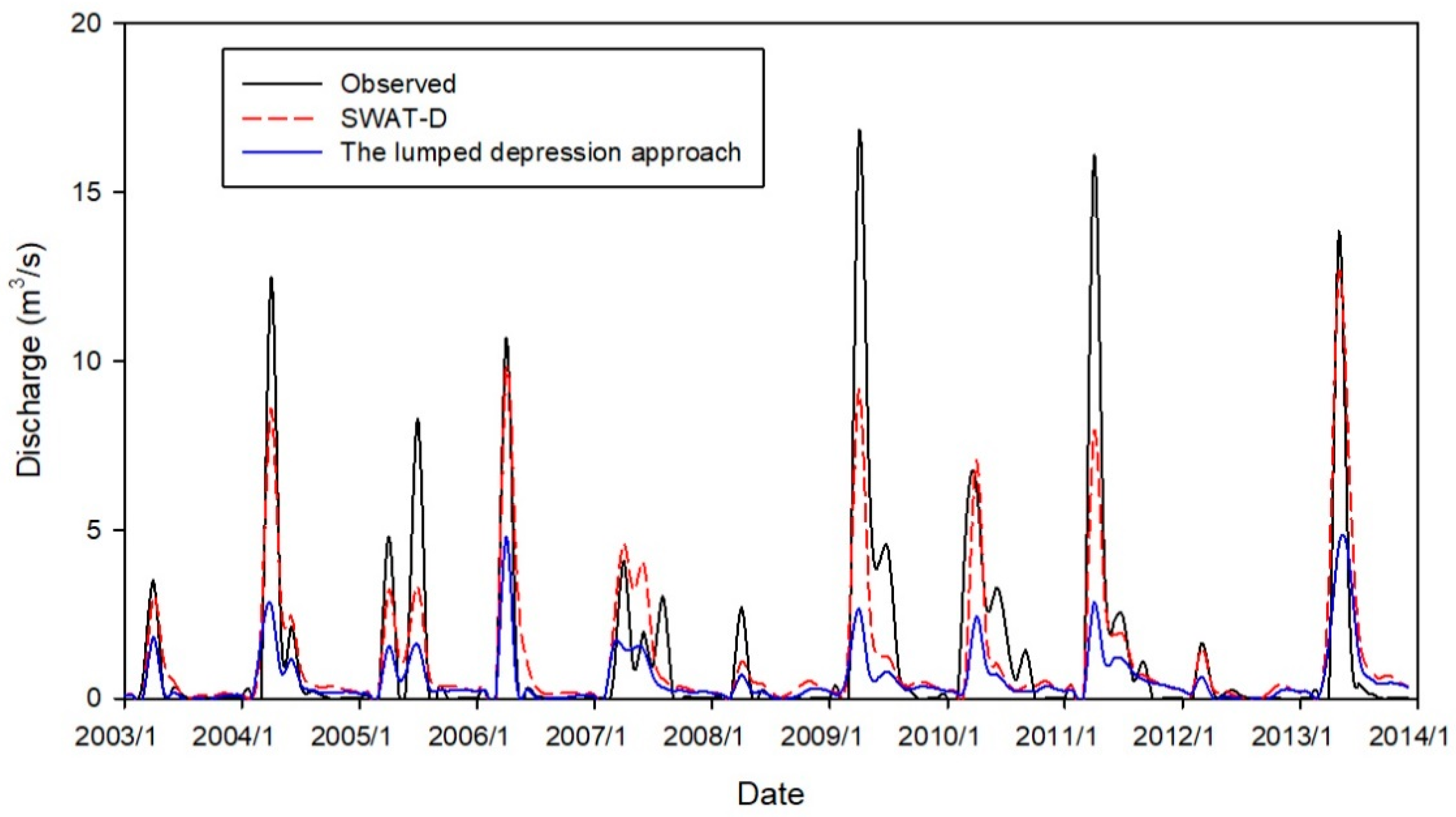
In the comparison of the simulated and observed outlet discharges, both the graphic comparison and statistic metrics showed the satisfactory performance of the SWAT-D. The simulated hydrograph at the watershed outlet followed the general shape of the observed hydrograph, and the magnitudes and distribution of most peak flows simulated by the SWAT-D matched the observed ones. The volumes of discharges during the simulation period can also be reproduced by the SWAT-D, with only a 7% deviation between the simulated and observed volume of discharges in 2004. The NSE values for the simulated monthly average discharges during calibration and validation periods were 0.78 and 0.71, respectively, indicating the ability of the SWAT-D in mimicking the threshold-controlled overland flow dynamics. In addition, the SWAT-D and the lumped depression approach were compared in terms of modeling methods and simulation results. The outlet discharges simulated by the SWAT-D and the lumped depression approach showed significant differences, which can be attributed to the different representations of the depressions. Aggregating all the depressions in the lumped depression approach tended to underestimate surface runoff and outlet discharges while tracking the filling–spilling dynamics of the depressions in the SWAT-D improved the simulation of the depression-influenced catchment responses. The modeling method of the SWAT-D was also compared with depression-dominated probability distribution models. The statistic estimation of subbasin-contributing areas in the probability distribution models leads to an insufficient characterization of depression-influenced hydrologic processes while tracking the filling–spilling of the depressions ensures that the SWAT-D can reproduce the intermittent, stepwise changes of subbasin-contributing areas.

While the SWAT-D was successfully applied to the Edmore Coulee watershed, it is expected in the future to test it for a variety of depression-dominated watersheds with subbasin-level observed data. Additionally, the SWAT-D can be further improved by considering more impact factors of hydrologic processes, such as the spatial distribution of depressions.

References

1. Arabi, M.; Govindaraju, R.; Sophocleous, M.; Koelliker, J. Use of distributed models for watershed management: Case studies. In Watershed Models; Taylor and Francis: Boca Raton, FL, USA, 2006. [Google Scholar]
2. Borah, D.K.; Bera, M. Watershed-scale hydrologic and nonpoint-source pollution models: Review of applications. Trans. ASABE 2004, 47, 789. [Google Scholar] [CrossRef] [Green Version]
3. Chourushi, S.; Lodha, P.P.; Prakash, I.A. Critical Review of Hydrological Modeling Practices for Flood Management. Pramana Res. J. 2019, 9, 352–362. [Google Scholar]
4. Daniel, E.B.; Camp, J.V.; LeBoeuf, E.J.; Penrod, J.R.; Abkowitz, M.D.; Dobbins, J.P. Watershed Modeling Using GIS Technology: A Critical Review. J. Spatial Hydrol. 2010, 10, 2. [Google Scholar]
5. Mekonnen, B.A.; Mazurek, K.A.; Putz, G. Incorporating landscape depression heterogeneity into the Soil and Water Assessment Tool (SWAT) using a probability distribution. Hydrol. Processes 2016, 30, 2373–2389. [Google Scholar] [CrossRef]
6. Rajib, A.; Golden, H.E.; Lane, C.R.; Wu, Q. Surface depression and wetland water storage improves major river basin hydrologic predictions. Water Resour. Res. 2020, 56, e2019WR026561. [Google Scholar] [CrossRef]
7. Tahmasebi Nasab, M.; Grimm, K.; Bazrkar, M.H.; Zeng, L.; Shabani, A.; Zhang, X.; Chu, X. SWAT modeling of non-point source pollution in depression-dominated basins under varying hydroclimatic conditions. Int. J. Environ. Res. Public Health 2018, 15, 2492. [Google Scholar] [CrossRef] [Green Version]
8. Amoah, J.K.O.; Amatya, D.M.; Nnaji, S. Quantifying watershed surface depression storage: Determination and application in a hydrologic model. Hydrol. Processes 2013, 27, 2401–2413. [Google Scholar] [CrossRef]
9. Arnold, J.G.; Srinivasan, R.; Muttiah, R.S.; Williams, J.R. Large Area Hydrologic Modeling and Assessment Part I: Model Development. J. Am. Water Resour. Assoc. 1998, 34, 73–89. [Google Scholar] [CrossRef]
10. Markstrom, S.L.; Regan, R.S.; Hay, L.E.; Viger, R.J.; Webb, R.M.; Payn, R.A.; LaFontaine, J.H. PRMS-IV, the precipitation-runoff modeling system, version 4. US Geol. Surv. Tech. Methods 2015, 6, B7. [Google Scholar]
11. Tahmasebi Nasab, M.; Singh, V.; Chu, X. SWAT Modeling for Depression-Dominated Areas: How Do Depressions Manipulate Hydrologic Modeling? Water 2017, 9, 58. [Google Scholar] [CrossRef] [Green Version]
12. Wang, X.; Yang, W.; Melesse, A.M. Using Hydrologic Equivalent Wetland Concept Within SWAT to Estimate Streamflow in Watersheds with Numerous Wetlands. Trans. ASABE 2008, 51, 55–72. [Google Scholar] [CrossRef]
13. Yang, W.; Wang, X.; Liu, Y.; Gabor, S.; Boychuk, L.; Badiou, P. Simulated environmental effects of wetland restoration scenarios in a typical Canadian prairie watershed. Wetl. Ecol. Manag. 2010, 18, 269–279. [Google Scholar] [CrossRef]
14. Antoine, M.; Javaux, M.; Bielders, C. What indicators can capture runoff-relevant connectivity properties of the micro-topography at the plot scale? Adv. Water Resour. 2009, 32, 1297–1310. [Google Scholar] [CrossRef]
15. Wang, N.; Zhang, X.; Chu, X. New model for simulating hydrologic processes under influence of surface depressions. J. Hydrol. Eng. 2019, 24, 04019008. [Google Scholar] [CrossRef]
16. Grimm, K.; Chu, X. Depression threshold control proxy to improve HEC-HMS modeling of depression-dominated watersheds. Hydrol. Sci. J. 2020, 65, 200–211. [Google Scholar] [CrossRef]
17. Le Phong, V.V.; Kumar Praveen, P. Power law scaling of topographic depressions and their hydrologic connectivity. Geophys. Res. Lett. 2014, 41, 1553–1559. [Google Scholar] [CrossRef]
18. Ullah, W.; Dickinson, W.T. Quantitative description of depression storage using a digital surface model: I. Determination of depression storage. J. Hydrol. 1979, 42, 63–75. [Google Scholar] [CrossRef]
19. Zeng, L.; Chu, X. A new Probability-Embodied model for simulating variable contributing areas and hydrologic processes dominated by surface depressions. J. Hydrol. 2021, 602, 126762. [Google Scholar] [CrossRef]
20. Zeng, L.; Chu, X. Integrating Depression Storages and their Spatial Distribution in Watershed-Scale Hydrologic Modeling. Adv. Water Resour. 2021, 151, 103911. [Google Scholar] [CrossRef]
21. Evenson, G.R.; Golden, H.E.; Lane, C.R.; D’Amico, E. Geographically isolated wetlands and watershed hydrology: A modified model analysis. J. Hydrol. 2015, 529, 240–256. [Google Scholar] [CrossRef] [Green Version]
22. Zeng, L.; Shao, J.; Chu, X. Improved hydrologic modeling in depression-dominated areas. J. Hydro. 2020, 590, 125269. [Google Scholar] [CrossRef]
23. Wang, N.; Chu, X. A new algorithm for delineation of surface depressions and channels. Water 2020, 12, 7. [Google Scholar] [CrossRef] [Green Version]
24. Chu, X.; Yang, J.; Zhang, J.; Chi, Y. An improved method for watershed delineation and computation of surface depression storage. In Watershed Management; American Society of Civil Engineers: Reston, VA, USA, 2010; pp. 1113–1122. [Google Scholar] [CrossRef]
25. Nasab, M.T.; Zhang, J.; Chu, X. A new depression-dominated delineation (D-cubed) method for improved watershed modelling. Hydrol. Processes 2017, 31, 3364–3378. [Google Scholar] [CrossRef]
26. Nash, J.E.; Sutcliffe, J.V. River flow forecasting through conceptual models part I: A discussion of principles. J. Hydrol. 1970, 10, 282–290. [Google Scholar] [CrossRef]
27. Gupta, H.; Sorooshian, S.; Yapo, P. Status of automatic calibration for hydrologic models: Comparison with multilevel expert calibration. J. Hydrol. Eng. 1999, 4, 135–143. [Google Scholar] [CrossRef]
28. Moriasi, D.N.; Arnold, J.G.; Van Liew, M.W.; Bingner, R.L.; Harmel, R.D.; Veith, T.L. Model evaluation guidelines for systematic quantification of accuracy in watershed simulations. Trans. ASABE 2007, 50, 885–900. [Google Scholar] [CrossRef]
29. Moriasi, D.N.; Zeckoski, R.W.; Arnold, J.G.; Baffaut, C.; Malone, R.W.; Daggupati, P.; Guzman, J.A.; Saraswat, D.; Yuan, Y.; Douglas-Mankin, K.R. Hydrologic and water quality models: Key calibration and validation topics. Trans. ASABE 2015, 58, 1609–1618. [Google Scholar] [CrossRef]
Figure 1. Example of the intrinsic changing patterns of the normalized contributing area and fully-filled depression storage.
Water 14 00652 g001
Figure 2. Flowchart of the SWAT-D model.
Water 14 00652 g002
Figure 3. Modeling of depression-oriented hydrologic processes in SWAT-D.
Water 14 00652 g003
Figure 4. Location of the Edmore Coulee watershed, watershed outlet, climate stations, and water bodies.
Water 14 00652 g004
Figure 5. Distributions of PBUs and CBUs of the watershed.
Water 14 00652 g005
Figure 6. Distributions of maximum depression storage of all subbasins (The boxplot shows the 10th percentile, 25th percentile, median, 75th percentile, and 90th percentile of the maximum depression storage).
Water 14 00652 g006
Figure 7. (a) Intrinsic changing patterns of contributing area for all subbasins, and (b) intrinsic changing patterns of depression storage of contributing area for all subbasins.
Water 14 00652 g007
Figure 8. Comparison of the simulated and observed monthly average flows at the watershed outlet.
Water 14 00652 g008
Figure 9. Comparison of the simulated and observed daily flows at the watershed outlet for (a) calibration period and (b) validation period.
Water 14 00652 g009
Figure 10. Comparison of two modeling methods (a) lumped depression approach and (b) SWAT-D.
Water 14 00652 g010