Turbulence Structure in a Stratocumulus Cloud


Department of Mechanical Engineering, University of Connecticut, Storrs, CT 06269, USA
Atmosphere 2018, 9(10), 392; https://doi.org/10.3390/atmos9100392
Submission received: 16 July 2018
/
Revised: 31 August 2018
/
Accepted: 17 September 2018
/
Published: 10 October 2018
(This article belongs to the Special Issue Large-Eddy Simulations (LES) of Atmospheric Boundary Layer Flows)
Abstract
:The growth of computing power combined with advances in modeling methods can yield high-fidelity simulations establishing numerical simulation as a key tool for discovery in the atmospheric sciences. A fine-scale large-eddy simulation (LES) utilizing 1.25 m grid resolution and horizontal domain is used to investigate the turbulence and liquid water structure in a stratocumulus cloud. The simulations capture the observed cloud morphology, including elongated regions of low liquid water path, cloud holes, and pockets of clear air within the cloud. The cloud can be partitioned into two broad layers with respect to the maximum mean liquid. The lower layer resembles convective turbulent structure with classical inertial range scaling of the velocity and scalar energy spectra. The top and shallower layer is directly influenced by the cloud top radiative cooling and the entrainment process. Near the cloud top, the liquid water spectra become shallower and transition to a power law for scales smaller than about .
1. Introduction
Stratocumulus clouds (Sc) cover about one-quarter of the Earth’s surface and have a large impact on the Earth’s radiative balance because they strongly reflect incoming solar radiation but they have a small effect on outgoing longwave radiation, e.g., [1,2,3,4]. In spite of the seeming simplicity of a “lumpy” low-cloud deck, it is challenging to quantify the properties of the cloud-topped atmospheric boundary layer given the large-scale meteorological conditions. A delicate balance of processes leads to difficulties in the formulation of accurate parameterizations for weather and climate models, e.g., [5,6,7].
Our understanding of the cloud-scale macrophysical and microphysical processes in stratocumulus topped boundary layers primarily derives from several observational campaigns, e.g., [8,9,10,11]. Because of the multiscale multiphysics character of the flow, the modeling and simulation of stratocumulus has been challenging, e.g., [12,13]. However, the growth of computing power combined with advances in modeling methods is yielding high-fidelity simulations establishing numerical simulation as a key tool for discovery in the atmospheric sciences.
The immense range of scales encountered in atmospheric boundary layer flows (approximately to several km) make simulation of all scales prohibitive in the foreseeable future, thus a significant subrange of the flow must be modeled by a suitable parameterization or turbulence closure. Large-eddy simulation is the most prominent high-resolution modeling methodology that explicitly resolves the dynamically important flow scales and models the smaller, more “generic” in nature, scales, e.g., [14,15].
Initially, LES closures were simple [16] and three-dimensional simulations very coarse [17]. However, the theoretical framework of the method improved [18,19,20,21] and efforts to better understand the performance of LES in atmospheric flows followed [22,23]. The premise and predictive power of the methodology relies on the reduction of the flow organization and structure at small scales. For instance, the resolved-scale dynamics capture the complex cloud shapes whereas the turbulence model represents the effects of stratified turbulence in a small volume (–) of the atmosphere.
Accordingly, the goal of the present paper is twofold: demonstrate the potential of the LES methodology as an essential tool for discovery in atmospheric science and, using one of largest LES performed to date, study the small-scale structure of a stratocumulus cloud. The very high resolution simulation (grid spacing is ) enables a fine-scale exploration of the spatial structure of the cloud morphology. The principal aspect of the present study is the study of the characteristics of the cloud liquid variability.
The case of a nocturnal stratocumulus corresponding to the first research flight (RF01) of the second Dynamics and Chemistry of Marine Stratocumulus (DYCOMS-II) field study [9] is simulated. The physical processes in the simulation include, in addition to turbulent transport in a stratified flow, vapor–liquid phase changes and longwave radiative transfer. The LES is validated using the DYCOMS-II RF01 in-situ observations [9,13].
2. Large-Eddy Simulation
2.1. Governing Equations
The LES model of [15] is used to simulate the nocturnal stratocumulus case of [13]. The Favre-filtered (density-weighted) anelastic approximation of the Navier–Stokes equations [24] is numerically integrated on an f-plane (). The filtered variables, are defined as , where is the density and the overbar denotes a spatially filtered variable. The conservation equations for mass, momentum, liquid water potential temperature, and total water, neglecting resolved-scale viscous terms, are, respectively,
The thermodynamic variables are decomposed into a constant potential temperature basic state, denoted by subscript 0, and a dynamic component. Accordingly, is the constant basic-state potential temperature and is the density. The Cartesian components of the velocity vector and geostrophic wind, are and , respectively, and is the Coriolis parameter, where the latitude is . Buoyancy is proportional to deviations of the virtual potential temperature, , from its instantaneous horizontal average, . The subgrid-scale (SGS) terms and are estimated using the buoyancy adjusted stretched-vortex SGS model [14].
The thermodynamic pressure, p, in each grid cell is computed from the sum of the basic state Exner function, , plus a contribution due to the deviation of the horizontal mean from the basic state, , and the dynamic part, , which enforces the anelastic constraint (1),
The effect of the large-scale environment is included in the equations for and through the subsidence terms, where is the uniform large-scale horizontal divergence. The liquid water potential temperature equation includes radiative heating and cooling through the net radiative flux, , divergence. The radiative flux is parameterized as in [13],
where
is the liquid water mixing ratio, and the column-wise inversion height. The values of the constants are , , m kg, and . The radiation parameterization causes strong cooling in a thin layer (∼10 m) at the cloud top and slight heating near the cloud base. The radiation flux is calculated at each model time step column-wise.
The amount of cloud water, , in each grid cell is estimated using an “all or nothing” saturation scheme, i.e., no partially saturated air in each grid cell. The thermodynamic state at the grid-cell center is used to classify each grid cell as saturated or clear and determine the corresponding thermodynamic coefficients for all variables, including those residing at the cell’s vertices. All water condensate is suspended, thus no drizzle/precipitation is allowed.
2.2. Boundary and Initial Conditions
The equations of motion are numerically integrated in a doubly periodic domain in the horizontal directions. The surface fluxes are dynamically computed in each grid cell using the Monin–Obukhov similarity theory (MOST) with Charnock’s roughness length parameterization [25]. A sea surface temperate is used [13], which results in similar mean sensible and latent heat fluxes, and , respectively, as in [13]. A Rayleigh damping layer is applied above , to limit gravity wave reflection.
The wind fields are initialized with the geostrophic wind, and and with a mixed layer–sharp inversion–free troposphere structure:
where is the initial boundary layer depth. Zero-mean random fluctuations are added to and at the lowermost to help quickly establish multiscale random convection after initialization.
2.3. Numerical Discretization
The governing Equations (1)–(4) are discretized on an Arakawa C (staggered) grid [26,27,28]. The fully conservative four-order advection scheme of [29] is used for momentum advection, the Quadratic Upstream Interpolation for Convective Kinematics (QUICK) [30] is used for and advection. QUICK does not enforce monotonicity (positive definiteness) of the advected scalar fields but it is less dissipative than monotone schemes, e.g., [31]. Second-order centered differences are used to approximate the spatial derivatives of the subgrid scale model terms. The semi-discrete system of equations is advanced in time using the third-order Runge–Kutta of [32]. Time integration is performed using a variable time step chosen such that the Courant–Friedrichs–Lewy (CFL) number is 1.2, resulting in a time step interval .
The grid is uniform and isotropic, i.e., , and the grid spacing is , with grid cells (about 20 billion total) in the horizontal and vertical directions, and domain. The simulation is one of the largest LES performed to date. The present simulation is a higher resolution complement to the series of lower resolution runs in [15]. Because the simulation is computationally challenging, it was ran only up to , instead of the typical . Comparisons of flow statistics between and using data from the run with show only small differences and no effects of the initial flow transient at .
The LES implementation is parallelized using a distributed memory paradigm with Message Passing Interface (MPI). The computational domain is partitioned using a two-dimensional decomposition in the horizontal directions, a typical choice for atmospheric models because several processes are performed column-wise, e.g., radiation in the present case. Thus, any such operation can be entirely computed using local data.
The simulation was carried out on the Pleiades computer at the NASA Advanced Supercomputing (NAS) Division at Ames Research Center using 256 Ivy Bridge nodes with 20 CPU-cores per node. Because at this (relatively small) number of nodes the simulation is memory limited, only 16 MPI ranks were launched per node, essentially utilizing only 16 of the 20 available CPU-cores, resulting in a total of 4096 MPI ranks. This configuration results in a wall-clock time of about per time step. 42,000 time steps were carried out to simulate the atmospheric boundary layer for of physical time. Even though the simulation is computationally expensive, modern computing platforms and programming methods result in relatively uncomplicated execution of the LES implementation. The greatest challenge is the analysis of the results because of the large data volume and the relatively slow read speed of the stored data.
3. Results
3.1. Boundary Layer Profiles and Validation
All flow statistics are computed from a single time instance of the simulation at . Mean profiles are horizontal averages at each model level. The estimates of the turbulent fluxes are composed of the resolved and SGS part, i.e., at model level k,
where i and j are the horizontal grid cell indexes and , the corresponding number of grid points. The SGS terms of the w triple correlation cannot be readily evaluated, thus only the resolved-scale part is used and the estimate is denoted by .
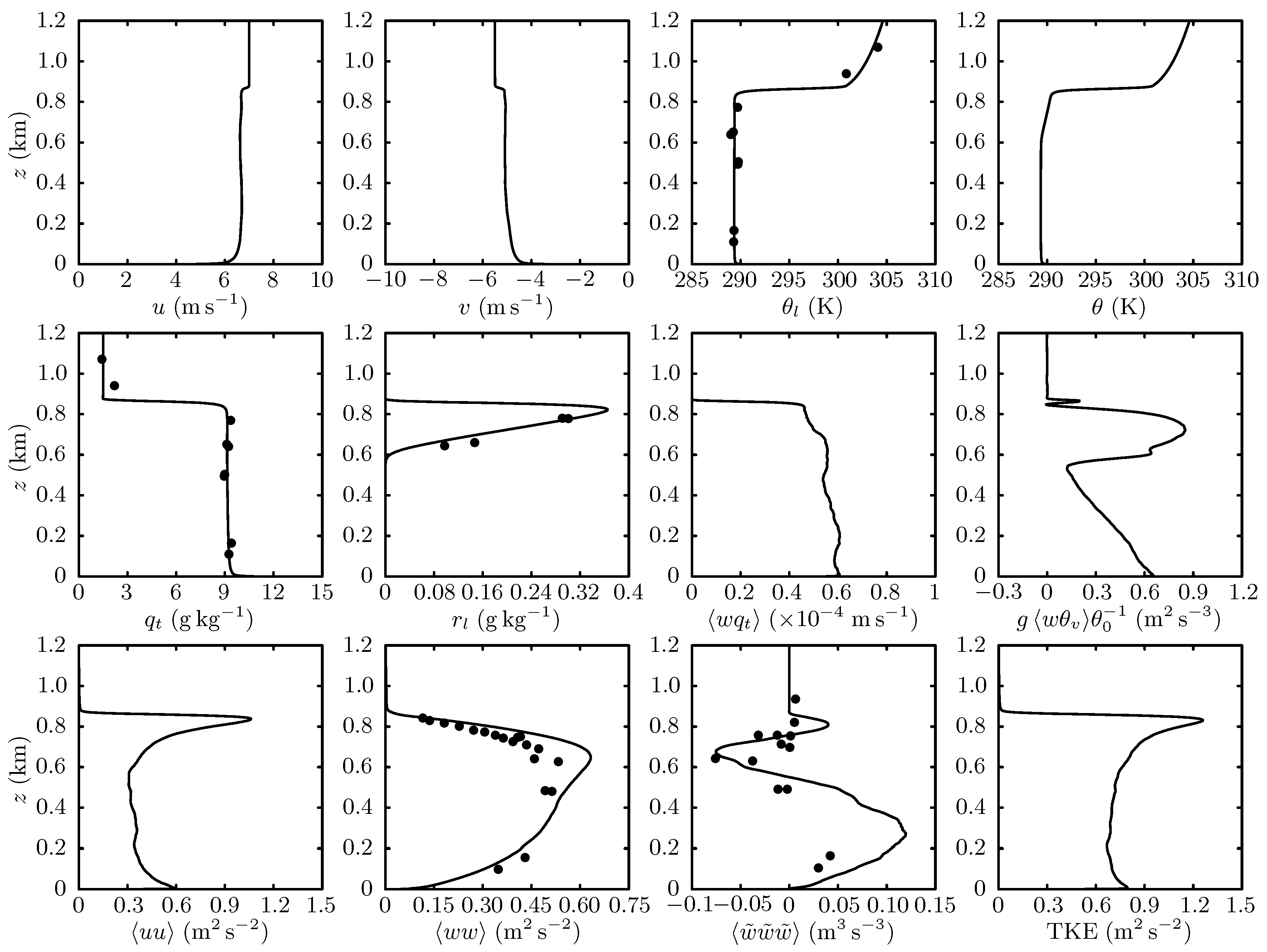
Figure 1 shows boundary layer profiles and compares the LES results with the observations [13]. Momentum and the conserved variables, and , are well mixed in the boundary layer. The buoyancy flux implies a coupled convection structure in the boundary layer since it attains a positive minimum value at cloud base [2]. Turbulent kinetic energy (TKE) and its components attain their highest values near the cloud top because of the buoyancy forcing of radiative cooling.
The LES results agree with observations and are grid converged with respect to a courser run at [15]. The largest difference with the coarser simulation is in the amount of cloud liquid with the present run having about 10% more liquid water path (LWP).
Most LES of DYCOMS-II RF01, even if they accurately capture the amount of cloud liquid [33,34], under-predict . Presently , , and agree with observations. The values are somewhat higher than the observations near the cloud top, but this is likely because the comparison is carried out at rather than . Based on the trend of a coarser run with [15], somewhat decreases with time and the agreement improves for .
Similar to other LES results [13,33], is positive below the inversion, whereas observations do not include positive values in the same region. The vertical velocity triple correlation can be related to the relative strength between updrafts and downdrafts. Kopec et al. [35] compare the sign of mean and median of and conclude that strong but narrow updrafts are present in the cloud. The profiles of updraft and downdraft area fractions and the decomposition of covariances for the present case are discussed in [36].
3.2. Cloud Structure
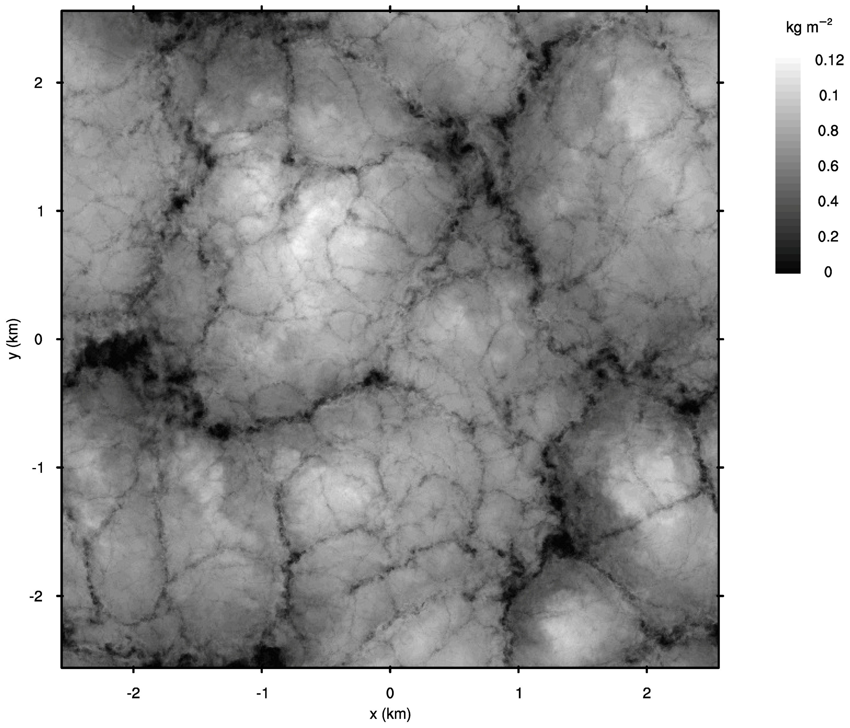
Previous studies of small-scale (1–) cloud liquid variability relied on in situ airborne measurements [37,38,39,40,41,42,43] or radar observations [44]. The observational data sets are either one dimensional (along flight paths) or two dimensional (z–t pairs in radar observations), thus the horizontal fine-scale variability of the cloud is not readily apparent. Figure 2 shows the rich multiscale structure of LWP in the LES. The characteristic “lumpy” structure of the cloud is interlaced with elongated regions of very low LWP.
In the LES a “cloudy,” i.e., saturated, grid cell is defined as any cell with , and a cloudy column as any column with at least one cloudy grid cell. Figure 2 shows that cloud cover fraction is nearly 100% with the darker contours corresponding to negligible LWP. High values of LWP correspond to the locations of updrafts that replenish the cloud water, as shown in the total water visualizations of [45].
The LWP contours in Figure 2 are consistent with observations, which also show a highly variable liquid water content (LWC) [40,41,43] suggesting a complex flow where both saturated and clear air regions can be encountered in the cloud layer. Direct numerical simulations (DNS) of stratocumulus cloud tops, e.g., Figure 3 of [46], also show clear air descending into the cloud. Presently, the goal is to exploit the availability of the three-dimensional flow field in the LES to complement the results of past observation-based investigations. The underlying problem of the spatial variability of the cloud liquid is challenging and connected to the geometry of the turbulent motions and the dynamics of the vapor–liquid system. Accordingly, several terms are used to describe these features, such as cloud holes, turbules, and wisps, see [40] and references therein.
A few simple metrics are presently used to describe the geometry of the cloud. Results are presented with respect to the mean cloud depth , which is defined as the depth of the mean profile, and the height of the maximum cloud liquid . Depth statistics are normalized with respect to and heights with respect to . The inversion height is defined as the height where the mean , which is about the mean of the mixed layer and free troposphere values. Table 1 summarizes the reference parameters and their values.
Two local column-wise cloud morphology metrics are defined. The total cloud depth,
where is the height of the lowermost cloudy grid cell and the height of the uppermost cloudy grid cell, if saturated grid cells are present in the column, otherwise . Within the vertical length not all grid cells are necessarily cloudy. Thus, the total cloud void depth is defined as
the cumulative height of the non saturated internal to cloud grid cells, where is the indicator function. The present definition of differs from the typical definition of cloud holes, e.g., Figure 2 of [40], because saturated air must be present at the top and bottom of the cloud void. In contrast, cloud holes are not necessarily enclosed within saturated air. The present definition is more representative of turbulent overturning events which can result in engulfment of clear air in the cloud, e.g., [47]. Moreover, is the total depth of one or more vertically overlapping regions.
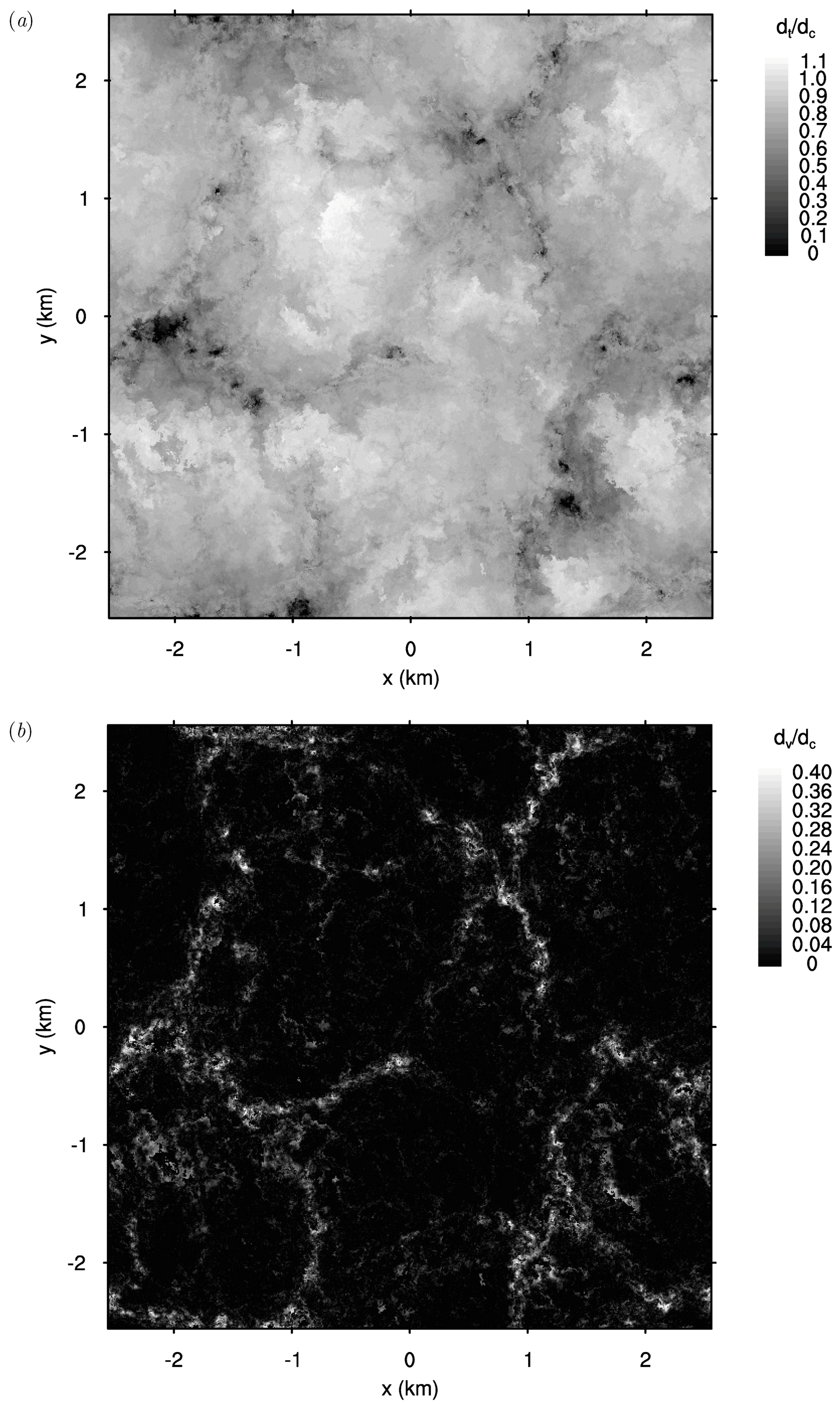
Figure 3 shows the normalized cloud depth, , and the total void depth, . A comparison between (Figure 3a) and LWP (Figure 2) shows that for many low LWP regions the cloudy column is deep. As shown in Figure 3a, the cloud fraction is nearly 100% with only a few locations where cloud holes reach the entire depth of the layer. Because is sensitive to overturning motions and engulfment of dry air into the cloud, it is expected to be an indicator of the structure of the entrainment events [48]. The highest values of are found around the cloud blobs suggesting that dry air can penetrate deep into the cloud, similar to DNS results [46]. In many instances the total clear air column height within the cloud is about a third of the mean cloud depth.
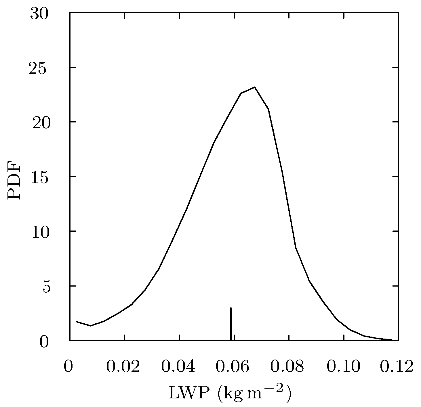
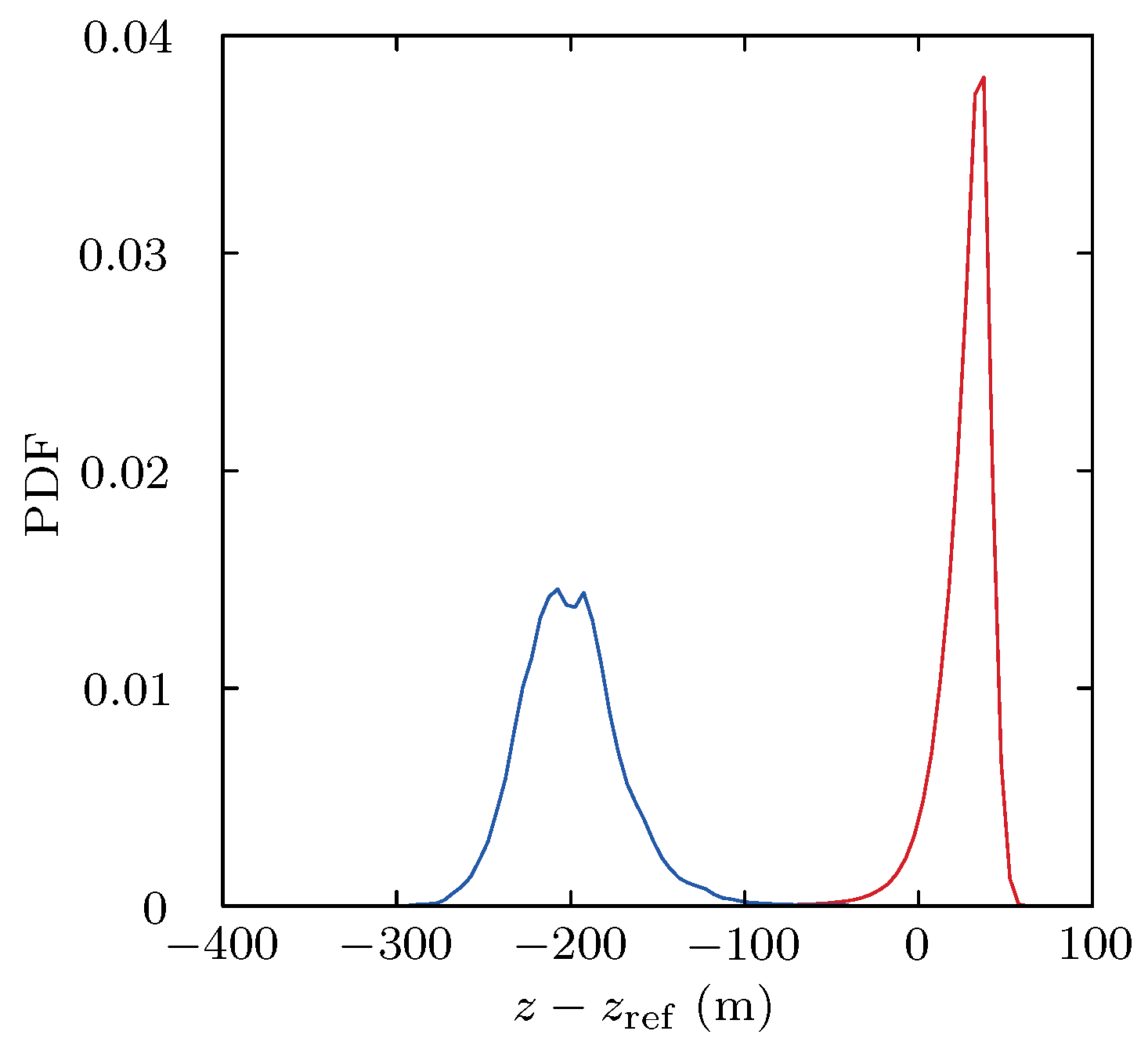
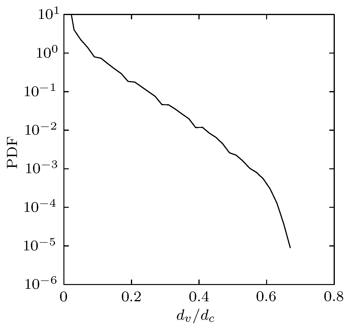
Whereas Figure 2 and Figure 3 explore the spatial structure of the cloud, Figure 4, Figure 5 and Figure 6 show the statistical distribution counterparts. Figure 4 shows the probability density function (PDF) of LWP, i.e., the normalized histogram. Figure 5 shows the PDF of the cloud base and cloud top heights with respect to the reference height and Figure 6 the PDF of the normalized total cloud void depth. Because most columns have low values, the PDF of is plotted in logarithmic scale.
The LWP PDF has negative skewness and similar shape to the reference case of [35]. The cloud base height PDF is much broader than the cloud top height PDF because moist updrafts tend to lower cloud base whereas dry downdrafts increase the cloud base height. The PDF is nearly symmetric similar to the PDF constructed from observations in [49]. The cloud top height PDF is asymmetric with a longer tail extending to lower z. Essentially, the entire PDF is confined to implying that the horizontal mean of increases below the inversion because of fluctuations of the cloud top. Interestingly, the PDF suggests that the large vertical length scales are present in the cloud-top motions. Accordingly, inviscid (large-scale) flow dynamics may primarily control stratocumulus entrainment, which in turn raises interesting questions regarding the extrapolation of DNS-derived scalings to cloud-scale entrainment rates, e.g., [50].
The PDF (Figure 6) exhibits nearly scaling, where c is a constant, for a wide range of . Because, only one condition is presently explored and given the variations in the LWP PDF in the numerical experiments of [35], it cannot be concluded that the observed PDF is characteristic of a broader range of stratocumulus.
3.3. Joint Probability Density Functions
The joint probability density functions (JPD) of the two conserved thermodynamic variables and , i.e., the buoyancy variable, versus vertical velocity are used to gain a fuller picture of the flow. Moreover, probability density functions are often used in modeling, e.g., [36,51,52,53,54,55].
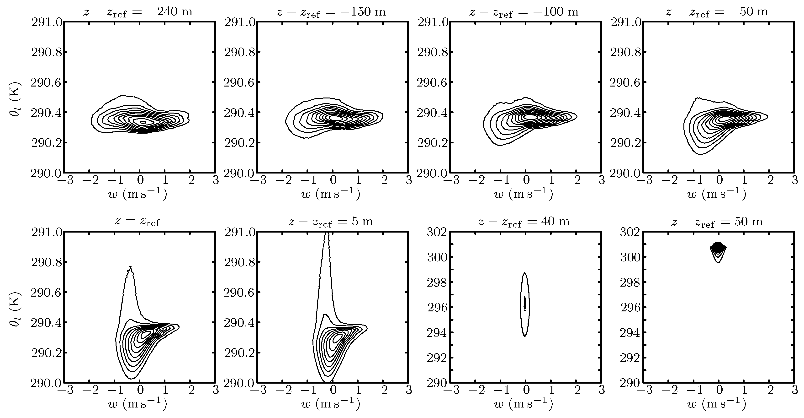
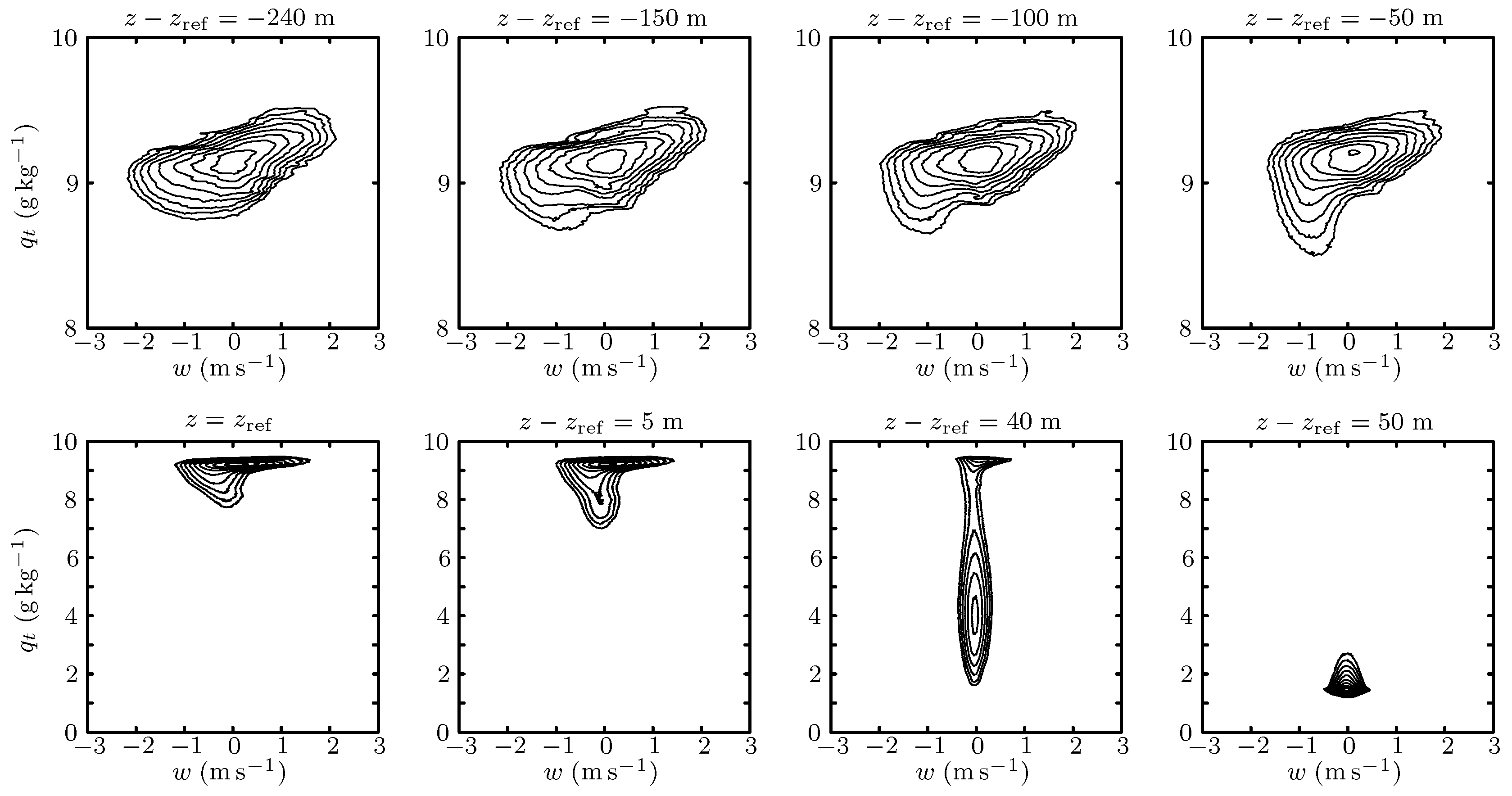
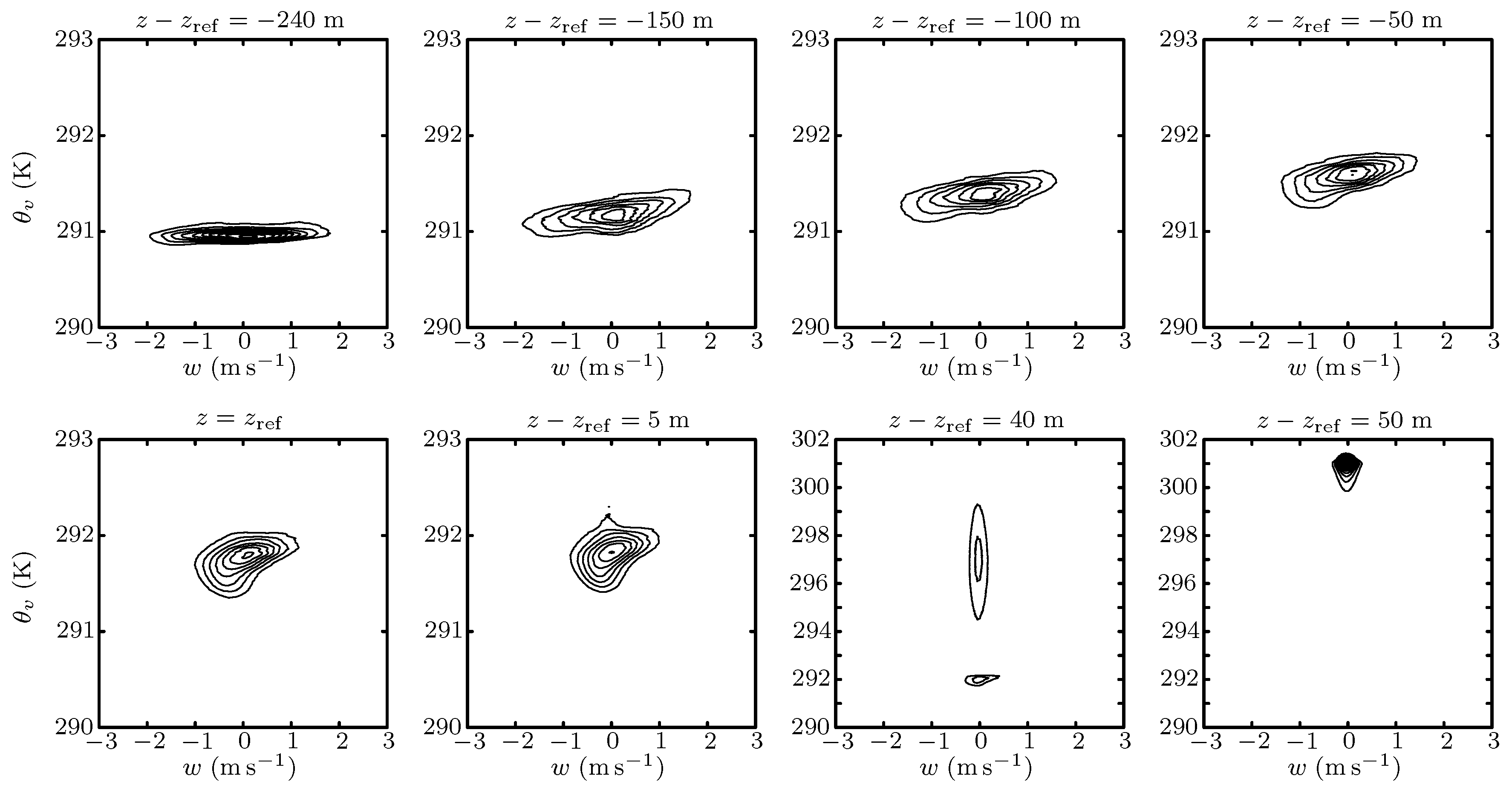
Figure 7, Figure 8 and Figure 9 show JPDs of –w, –w, and –w at various heights. The JPDs and spectra, in the following section, are computed at eight heights: four between cloud base and the maximum of the cloud liquid, , , , and , at the height of cloud liquid maximum ; and at , 40, and , between the maximum liquid amount height and cloud top. The JPDs were constructed similarly to [36] using data from all grid cells at the corresponding model level. Because most of the covariance is contributed by the “tails” of the JPD, in Figure 7, Figure 8 and Figure 9 the contours are plotted in logarithmic scale, i.e., the contours correspond to , where is the JPD.
For all JPDs show typical convection characteristics with an approximate joint Gaussian shape [36,51]. The influence of entrainment of free-tropospheric air is first observed at . In a thin layer of approximately the JPDs transition from their boundary layer values to zero-covariance free tropospheric JPDs. At about the JPDs are double peaked (not shown in the w– JPD contours of Figure 7). The vertical velocity distribution width decreases significantly for and the JPDs become narrower in the w coordinate, c.f., profiles in Figure 1.
Even though and w are somewhat correlated in the minor axis of the JPDs is broad. The correlation between buoyancy and vertical velocity becomes smaller for , suggesting that inertial and pressure contributions are also significant near the cloud top corroborating the results of [47].
3.4. Spectra
Turbulence spectra in stratocumulus clouds are discussed in the observation-based studies of [11,37,38,39,47,49] and in the LES of [12,47,56,57]. Spectra derived from previous LES do not show any well defined power law scaling, likely because of the coarse resolution and the narrow range of scales. Spectra from observations are often of liquid water fluctuations typically measured with respect to time. Spectra computed from observations exhibit scaling or a smaller in absolute value exponent depending on the scale, where k is a one-dimensional wavenumber [38,39,49]. There is no established theoretical prediction for the spectral scaling because the flow is stratified, the conserved scalars (presently, and ) are active scalars with strong contributions to buoyancy, whereas liquid water can be created or depleted (condensation/evaporation) with regions of no liquid (e.g., cloud voids).
Radial spectra of u, w, , and are computed from the LES by taking the two-dimensional Fourier transform, e.g., for , and then averaging across radial wavenumber “shells” to form . The x-axis in Figure 10, Figure 11 and Figure 12 is converted to length scale to help the interpretation and comparison to previous studies [38,39].
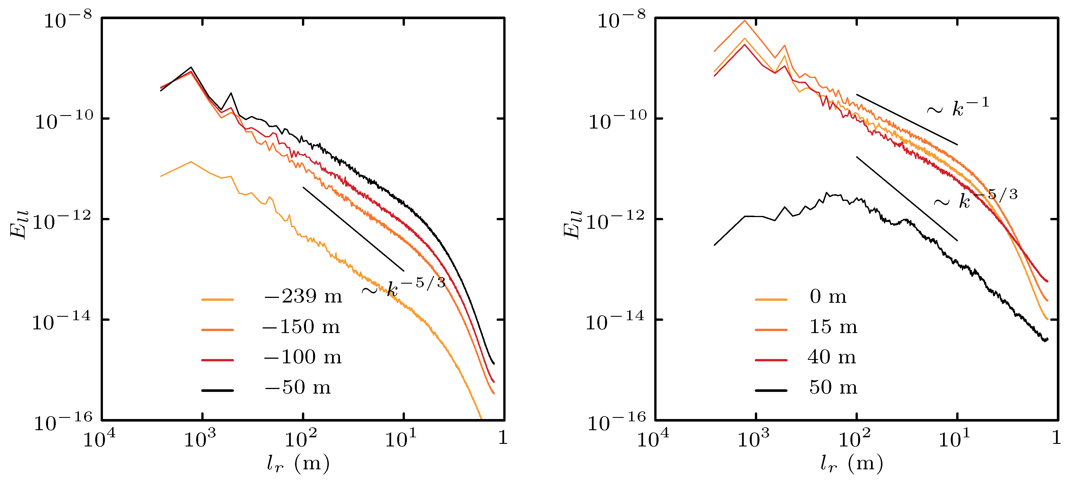
Figure 10 shows the spectra of u, w, and and Figure 11 the spectra of . The spectra are partitioned into two groups based on height with respect to . In Figure 10, the spectra at half boundary layer height are also plotted for reference. The spectra of u, w, and for are similar to the corresponding spectrum below cloud base and velocity and spectra show a well defined inertial range. The exponent is for the velocity components, similar to the Physics of Stratocumulus Top (POST) observations [11], and somewhat smaller in absolute value for . The constant exponent scaling extends to about 2.5 decades of scales. Temperature spectra of the POST observations show the opposite trend with higher in absolute value exponent values than when spectral energy is plotted in the frequency domain [58]. All spectra decrease quickly at small scales because of the implicit filtering property of the finite difference schemes, e.g., [59]. exhibits a constant exponent scaling below cloud base, however, as z increases the spectra develop curvature in the log–log coordinates of Figure 10. For the spectra of u, w, and constant-exponent scaling is not observed for , likely because of the entrainment of non-turbulent free-tropospheric air.
Liquid water spectra at all heights show nearly constant-exponent scaling. The exponent is near the cloud top and increases in absolute value as z decreases approaching near cloud base. Observations show scaling at scales larger than a few meters and a transition to a shallower spectrum at smaller scales [38]. Within the relatively narrow range of scales captured by the present LES, such a scale break in the liquid water spectra is not observed. Interestingly, at the cloud top exhibits ∼, however as can be inferred from the PDF (Figure 5), large cloud-free areas are expected, thus the exponent is likely not because of the presence of classical fully developed turbulence.
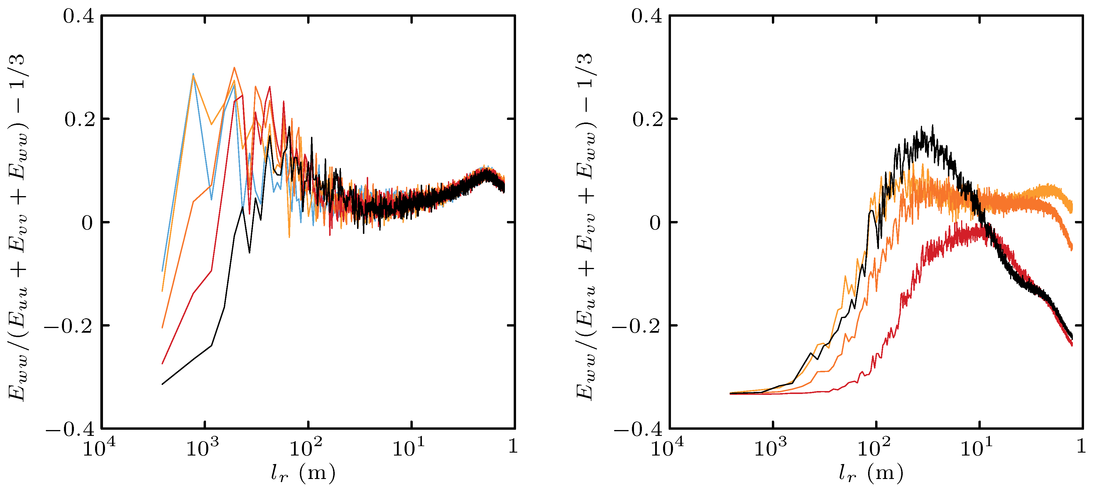
The anisotropy of the flow with respect to length scale is quantified using the velocity-anisotropy parameter , e.g., [60], which is similar to the parameter used in [57]. The velocity-anisotropy parameter is shown in Figure 12 at the same heights as the spectra in Figure 10 with parameter values near zero corresponding to an isotropic flow. At heights less than the anisotropy parameter is largely independent of height with motions being approximately isotropic for length scales less than . Overall, the present results are consistent with the analysis of the DYCOMS II RF01 observations and previous simulations [57]. The present results suggest that the flow is more isotropic at compared to [57].
4. Conclusions
The structure of turbulence and liquid water in a stratocumulus cloud is explored using a fine-scale large-eddy simulation (LES) utilizing 1.25 m grid resolution and horizontal domain. The simulation corresponds to the case of a nocturnal stratocumulus cloud observed during the first research flight of the DYCOMS-II field campaign [13]. The LES agrees with the observations including the variance and triple correlation of the vertical velocity, which are challenging to predict.
The simulations capture the observed cloud morphology, including elongated regions of low liquid water path (LWP), cloud holes, and pockets of clear air within the cloud. Comparisons between the spatial structure of LWP, cloud thickness, and total cloud void depth show regions of low cloud liquid and presence of clear (not saturated) air within the cloud at the boundaries of the cellular-like cloud “blobs.”
The cloud can be partitioned into two broad layers with respect to the height of maximum mean liquid. The lower layer resembles convective turbulent structure with approximately joint Gaussian probability density distributions of vertical velocity versus thermodynamic variables, classical inertial range scaling of the velocity spectra, and similar velocity anisotropy with respect to length scale. The top and shallower layer is directly influenced by the cloud top radiative cooling and the entrainment process. Near the cloud top the liquid water spectra become shallower and transition to a power law for scales smaller than about .
Overall, the LES captures fine details of the cloud structure across three decades of spatial scales demonstrating the key role of modeling and simulation in the atmospheric sciences. An important advantage of the simulations is the control of the meteorological conditions, which is difficult to achieve in observations as the actual atmosphere is often variable. However, the specification of the large-scale environment implies a degree of idealization in the typical LES setup, e.g., periodic boundary conditions in the horizontal directions, which can challenge the comparison between model and reality. The present model setup neglects any microphysical processes, such as drizzle, that can be important in some stratocumulus cloud regimes, e.g., [61]. Future simulations will include more physical processes further increasing the realism and value of modeling.
Funding
This research received no external funding.
Acknowledgments
Computational resources supporting this work were provided by the NASA High-End Computing (HEC) Program through the NASA Advanced Supercomputing (NAS) Division at Ames Research Center. The research presented in this paper was supported by the systems, services, and capabilities provided by the University of Connecticut High Performance Computing (HPC) facility. The article was improved by the comments of two anonymous reviewers.
Conflicts of Interest
The author declares no conflict of interest.
References
- Hartmann, D.L.; Ockert-Bell, M.E.; Michelsen, M.L. The effect of cloud type on Earth’s energy balance: Global analysis. J. Clim. 1992, 5, 1281–1304. [Google Scholar] [CrossRef]
- Bretherton, C.S. Convection in stratocumulus-topped atmospheric boundary layers. In The Physics and Parameterization of Moist Atmospheric Convection; Springer: Dordrecht, Germany, 1997; pp. 127–142. [Google Scholar]
- Stevens, B. Atmospheric moist convection. Annu. Rev. Earth Planet. Sci. 2005, 33, 605–643. [Google Scholar] [CrossRef]
- Wood, R. Stratocumulus clouds. Mon. Weather Rev. 2012, 140, 2373–2423. [Google Scholar] [CrossRef]
- Bony, S.; Dufresne, J.L. Marine boundary layer clouds at the heart of tropical cloud feedback uncertainties in climate models. Geophys. Res. Lett. 2005, 32, L20806. [Google Scholar] [CrossRef]
- Bretherton, C.S. Insights into low-latitude cloud feedbacks from high-resolution models. Philos. Trans. R. Soc. A 2015, 373, 20140415. [Google Scholar] [CrossRef] [PubMed]
- Tsushima, Y.; Ringer, M.A.; Koshiro, T.; Kawai, H.; Roehrig, R.; Cole, J.; Watanabe, M.; Yokohata, T.; Bodas-Salcedo, A.; Williams, K.D.; et al. Robustness, uncertainties, and emergent constraints in the radiative responses of stratocumulus cloud regimes to future warming. Clim. Dyn. 2016, 46, 3025–3039. [Google Scholar] [CrossRef]
- Lenschow, D.H.; Paluch, I.R.; Bandy, A.R.; Pearson, R., Jr.; Kawa, S.R.; Weaver, C.J.; Huebert, B.J.; Kay, J.G.; Thornton, D.C.; Driedger, A.R., III. Dynamics and chemistry of marine stratocumulus (DYCOMS) Experiment. Bull. Am. Meteor. Soc. 1988, 69, 1058–1067. [Google Scholar] [CrossRef]
- Stevens, B.; Lenschow, D.H.; Vali, G.; Gerber, H.; Bandy, A.; Blomquist, B.; Brenguier, J.; Bretherton, C.; Burnet, F.; Campos, T.; et al. Dynamics and chemistry of marine stratocumulus—DYCOMS-II. Bull. Am. Meteorol. Soc. 2003, 84, 579–593. [Google Scholar] [CrossRef]
- Gerber, H.; Frick, G.; Malinowski, S.P.; Jonsson, H.; Khelif, D.; Krueger, S.K. Entrainment rates and microphysics in POST stratocumulus. J. Geophys. Res. Atmos. 2013, 118, 12-094. [Google Scholar] [CrossRef]
- Plante, J.L.; Ma, Y.F.; Nurowska, K.; Gerber, H.; Khelif, D.; Karpinska, K.; Kopec, M.K.; Kumala, W.; Malinowski, S.P. Physics of Stratocumulus Top (POST): Turbulence characteristics. Atmos. Chem. Phys. 2016, 16, 9711–9725. [Google Scholar] [CrossRef]
- Stevens, D.E.; Bell, J.B.; Almgren, A.S.; Beckner, V.E.; Rendleman, C.A. Small-scale processes and entrainment in a stratocumulus marine boundary layer. J. Atmos. Sci. 2000, 57, 567–581. [Google Scholar] [CrossRef]
- Stevens, B.; Moeng, C.H.; Ackerman, A.S.; Bretherton, C.S.; Chlond, A.; DeRoode, S.; Edwards, J.; Golaz, J.C.; Jiang, H.L.; Khairoutdinov, M.; et al. Evaluation of large-eddy simulations via observations of nocturnal marine stratocumulus. Mon. Weather Rev. 2005, 133, 1443–1462. [Google Scholar] [CrossRef]
- Chung, D.; Matheou, G. Large-eddy simulation of stratified turbulence. Part I: A vortex-based subgrid-scale model. J. Atmos. Sci. 2014, 71, 1863–1879. [Google Scholar] [CrossRef]
- Matheou, G.; Chung, D. Large-eddy simulation of stratified turbulence. Part II: Application of the stretched-vortex model to the atmospheric boundary layer. J. Atmos. Sci. 2014, 71, 4439–4460. [Google Scholar] [CrossRef]
- Smagorinsky, J. General circulation experiments with the primitive equations. I. The basic experiment. Mon. Weather Rev. 1963, 91, 99–164. [Google Scholar] [CrossRef]
- Deardorff, J.W. A numerical study of three-dimensional turbulent channel flow at large Reynolds numbers. J. Fluid Mech. 1970, 41, 453–480. [Google Scholar] [CrossRef]
- Lilly, D.K. The representation of small-scale turbulence in numerical simulation experiments. In IBM Scientific Computing Symposium on Environmental Sciences; IBM: Yorktown Heights, NY, USA, 1967; pp. 195–210. [Google Scholar]
- Deardorff, J. On the magnitude of the subgrid scale eddy coefficient. J. Comput. Phys. 1971, 7, 120–133. [Google Scholar] [CrossRef]
- Leonard, A. Energy cascade in large-eddy simulations of turbulent fluid flows. Adv. Geophys. 1974, 18, 237–248. [Google Scholar]
- Smagorinsky, J. Some historical remarks on the use of nonlinear viscosities. In Large Eddy Simulation of Complex Engineering and Geophysical Flows; Galperin, B., Orszag, S.A., Eds.; Cambridge University Press: New York, NY, USA, 1993; pp. 3–36. [Google Scholar]
- Brown, A.R. The sensitivity of large-eddy simulations of shallow cumulus convection to resolution and subgrid model. Q. J. R. Meteorol. Soc. 1999, 125, 469–482. [Google Scholar] [CrossRef]
- Stevens, B.; Moeng, C.H.; Sullivan, P.P. Large-eddy simulations-of radiatively driven convection: Sensitivities to the representation of small scales. J. Atmos. Sci. 1999, 56, 3963–3984. [Google Scholar] [CrossRef]
- Ogura, Y.; Phillips, N.A. Scale analysis of deep and shallow convection in the atmosphere. J. Atmos. Sci. 1962, 19, 173–179. [Google Scholar] [CrossRef]
- Charnock, H. Wind stress over a water surface. Q. J. R. Meteorol. Soc. 1955, 81, 639–640. [Google Scholar] [CrossRef]
- Harlow, F.H.; Welch, J.E. Numerical calculation of time-dependent viscous incompressible flow of fluid with free surface. Phys. Fluids 1965, 8, 2182–2189. [Google Scholar] [CrossRef]
- Arakawa, A.; Lamb, V.R. Computational design of the basic dynamical processes of the UCLA general circulation model. In Methods of Computational Physics; Academic Press: New York, NY, USA, 1977; Volume 17, pp. 173–265. [Google Scholar]
- Matheou, G.; Chung, D.; Nuijens, L.; Stevens, B.; Teixeira, J. On the fidelity of large-eddy simulation of shallow precipitating cumulus convection. Mon. Weather Rev. 2011, 139, 2918–2939. [Google Scholar] [CrossRef]
- Morinishi, Y.; Lund, T.S.; Vasilyev, O.V.; Moin, P. Fully conservative higher order finite difference schemes for incompressible flow. J. Comput. Phys. 1998, 143, 90–124. [Google Scholar] [CrossRef]
- Leonard, B.P. A stable and accurate convective modelling procedure based on quadratic upstream interpolation. Comput. Methods Appl. Mech. Eng. 1979, 19, 59–98. [Google Scholar] [CrossRef]
- Matheou, G.; Dimotakis, P.E. Scalar excursions in large-eddy simulations. J. Comput. Phys. 2016, 327, 97–120. [Google Scholar] [CrossRef] [Green Version]
- Spalart, P.R.; Moser, R.D.; Rogers, M.M. Spectral methods for the Navier–Stokes equations with one infinite and two periodic directions. J. Comput. Phys. 1991, 96, 297–324. [Google Scholar] [CrossRef]
- Yamaguchi, T.; Randall, D.A. Large-eddy simulation of evaporatively driven entrainment in cloud-topped mixed layers. J. Atmos. Sci. 2008, 65, 1481–1504. [Google Scholar] [CrossRef]
- Pressel, K.G.; Mishra, S.; Schneider, T.; Kaul, C.M.; Tan, Z. Numerics and subgrid-scale modeling in large eddy simulations of stratocumulus clouds. J. Adv. Model. Earth Syst. 2017, 9, 1342–1365. [Google Scholar] [CrossRef] [PubMed] [Green Version]
- Kopec, M.K.; Malinowski, S.P.; Piotrowski, Z.P. Effects of wind shear and radiative cooling on the stratocumulus-topped boundary layer. Q. J. R. Meteorol. Soc. 2016, 142, 3222–3233. [Google Scholar] [CrossRef]
- Chinita, M.J.; Matheou, G.; Teixeira, J. A joint probability density-based decomposition of turbulence in the atmospheric boundary layer. Mon. Weather Rev. 2018, 146, 503–523. [Google Scholar] [CrossRef]
- Nicholls, S. The structure of radiatively driven convection in stratocumulus. Q. J. R. Meteorol. Soc. 1989, 115, 487–511. [Google Scholar] [CrossRef]
- Davis, A.B.; Marshak, A.; Gerber, H.; Wiscombe, W.J. Horizontal structure of marine boundary layer clouds from centimeter to kilometer scales. J. Geophys. Res. Atmos. 1999, 104, 6123–6144. [Google Scholar] [CrossRef] [Green Version]
- Gerber, H.; Jensen, J.B.; Davis, A.B.; Marshak, A.; Wiscombe, W.J. Spectral density of cloud liquid water content at high frequencies. J. Atmos. Sci. 2001, 58, 497–503. [Google Scholar] [CrossRef]
- Gerber, H.; Frick, G.; Malinowski, S.P.; Brenguier, J.L.; Burnet, F. Holes and entrainment in stratocumulus. J. Atmos. Sci. 2005, 62, 443–459. [Google Scholar] [CrossRef]
- Haman, K.E.; Malinowski, S.P.; Kurowski, M.J.; Gerber, H.; Brenguier, J.L. Small scale mixing processes at the top of a marine stratocumulus—A case study. Q. J. R. Meteorol. Soc. 2007, 133, 213–226. [Google Scholar] [CrossRef]
- Malinowski, S.; Haman, K.; Kopec, M.; Kumala, W.; Gerber, H. Small-scale turbulent mixing at stratocumulus top observed by means of high resolution airborne temperature and LWC measurements. J. Phys. Conf. Ser. 2011, 318, 072013. [Google Scholar] [CrossRef] [Green Version]
- Malinowski, S.P.; Gerber, H.; Plante, J.L.; Kopec, M.K.; Kumala, W.; Nurowska, K.; Chuang, P.Y.; Khelif, D.; Haman, K.E. Physics of Stratocumulus Top (POST): Turbulent mixing across capping inversion. Atmos. Chem. Phys. 2013, 13, 12171–12186. [Google Scholar] [CrossRef]
- Kollias, P.; Albrecht, B. The turbulence structure in a continental stratocumulus cloud from millimeter-wavelength radar observations. J. Atmos. Sci. 2000, 57, 2417–2434. [Google Scholar] [CrossRef]
- Matheou, G.; Chung, D.; Teixeira, J. Large-eddy simulation of a stratocumulus cloud. Phys. Rev. Fluids 2017, 2, 090509. [Google Scholar] [CrossRef]
- Mellado, J.P. Cloud-top entrainment in stratocumulus clouds. Annu. Rev. Fluid Mech. 2017, 49, 145–169. [Google Scholar] [CrossRef]
- Yamaguchi, T.; Randall, D.A. Cooling of entrained parcels in a large-eddy simulation. J. Atmos. Sci. 2012, 69, 1118–1136. [Google Scholar] [CrossRef]
- Haman, K.E. Simple approach to dynamics of entrainment interface layers and cloud holes in stratocumulus clouds. Q. J. R. Meteorol. Soc. 2009, 135, 93–100. [Google Scholar] [CrossRef] [Green Version]
- Wood, R.; Taylor, J.P. Liquid water path variability in unbroken marine stratocumulus cloud. Q. J. R. Meteorol. Soc. 2001, 127, 2635–2662. [Google Scholar] [CrossRef]
- de Lozar, A.; Mellado, J.P. Mixing driven by radiative and evaporative cooling at the stratocumulus top. J. Atmos. Sci. 2015, 72, 4681–4700. [Google Scholar] [CrossRef]
- Wyngaard, J.C.; Moeng, C.H. Parameterizing turbulent diffusion through the joint probability density. Bound. Layer Meteorol. 1992, 60, 1–13. [Google Scholar] [CrossRef]
- Wang, S.; Stevens, B. Top-hat representation of turbulence statistics in cloud-topped boundary layers: A large eddy simulation study. J. Atmos. Sci. 2000, 57, 423–441. [Google Scholar] [CrossRef]
- Golaz, J.C.; Larson, V.E.; Cotton, W.R. A PDF-based model for boundary layer clouds. Part I: Method and model description. J. Atmos. Sci. 2002, 59, 3540–3551. [Google Scholar] [CrossRef]
- Larson, V.E.; Golaz, J.C. Using probability density functions to derive consistent closure relationships among higher-order moments. Mon. Weather Rev. 2005, 133, 1023–1042. [Google Scholar] [CrossRef]
- Bogenschutz, P.A.; Krueger, S.K. A simplified PDF parameterization of subgrid-scale clouds and turbulence for cloud-resolving models. J. Adv. Model. Earth Syst. 2013, 5, 195–211. [Google Scholar] [CrossRef] [Green Version]
- Pedersen, J.G.; Malinowski, S.P.; Grabowski, W.W. Resolution and domain-size sensitivity in implicit large-eddy simulation of the stratocumulus-topped boundary layer. J. Adv. Model. Earth Syst. 2016, 8, 885–903. [Google Scholar] [CrossRef] [Green Version]
- Pedersen, J.G.; Ma, Y.F.; Grabowski, W.W.; Malinowski, S.P. Anisotropy of observed and simulated turbulence in marine stratocumulus. J. Adv. Model. Earth Syst. 2018, 10, 500–515. [Google Scholar] [CrossRef]
- Ma, Y.F.; Malinowski, S.P.; Karpińska, K.; Gerber, H.E.; Kumala, W. Scaling analysis of temperature and liquid water content in the marine boundary layer clouds during POST. J. Atmos. Sci. 2017, 74, 4075–4092. [Google Scholar] [CrossRef]
- Matheou, G. Numerical discretization and subgrid-scale model effects on large-eddy simulations of a stable boundary layer. Q. J. R. Meteorol. Soc. 2016, 142, 3050–3062. [Google Scholar] [CrossRef]
- Chung, D.; Pullin, D.I. Direct numerical simulation and large-eddy simulation of stationary buoyancy-driven turbulence. J. Fluid Mech. 2010, 643, 279–308. [Google Scholar] [CrossRef]
- Stevens, B.; Vali, G.; Comstock, K.; Wood, R.; vanZanten, M.C.; Austin, P.H.; Bretherton, C.S.; Lenschow, D.H. Pockets of open cells and drizzle in marine stratocumulus. Bull. Am. Meteor. Soc. 2005, 86, 51–57. [Google Scholar] [CrossRef]
Figure 1.
Boundary layer profiles at . Lines correspond to the LES results and circles to observations. The turbulent fluxes include the subgrid contribution. The triple correlation of the vertical velocity is estimated only from the resolved-scaled field.
Figure 1.
Boundary layer profiles at . Lines correspond to the LES results and circles to observations. The turbulent fluxes include the subgrid contribution. The triple correlation of the vertical velocity is estimated only from the resolved-scaled field.

Figure 2.
Cloud liquid water path.

Figure 3.
(a) Cloud thickness and (b) total height of cloud voids . Both and are normalized by the cloud mean thickness .
Figure 3.
(a) Cloud thickness and (b) total height of cloud voids . Both and are normalized by the cloud mean thickness .

Figure 4.
Probability density function of liquid water path. The vertical line corresponds to the mean LWP.
Figure 4.
Probability density function of liquid water path. The vertical line corresponds to the mean LWP.

Figure 5.
Probability density functions of cloud base and cloud top heights with respect to the height of the maximum mean cloud liquid .
Figure 5.
Probability density functions of cloud base and cloud top heights with respect to the height of the maximum mean cloud liquid .

Figure 6.
Distribution of normalized total height of cloud voids.

Figure 7.
Joint probability density functions of liquid water potential temperature and vertical velocity. Each panel corresponds to different height. The heights are with respect to the height of the maximum mean cloud liquid . The contours are plotted in logarithmic intervals.
Figure 7.
Joint probability density functions of liquid water potential temperature and vertical velocity. Each panel corresponds to different height. The heights are with respect to the height of the maximum mean cloud liquid . The contours are plotted in logarithmic intervals.

Figure 8.
Joint probability density functions of total water mixing ratio and vertical velocity. Each panel corresponds to different height. The heights are with respect to the height of the maximum mean cloud liquid . The contours are plotted in logarithmic intervals.
Figure 8.
Joint probability density functions of total water mixing ratio and vertical velocity. Each panel corresponds to different height. The heights are with respect to the height of the maximum mean cloud liquid . The contours are plotted in logarithmic intervals.

Figure 9.
Joint probability density functions of virtual potential temperature and vertical velocity. Each panel corresponds to different height. The heights are with respect to the height of the maximum mean cloud liquid . The contours are plotted in logarithmic intervals.
Figure 9.
Joint probability density functions of virtual potential temperature and vertical velocity. Each panel corresponds to different height. The heights are with respect to the height of the maximum mean cloud liquid . The contours are plotted in logarithmic intervals.

Figure 10.
Radial spectra of (top to bottom rows) zonal wind, vertical velocity, liquid water potential temperature, and total water mixing ratio. The legend denotes heights with respect to the height of the maximum mean cloud liquid . Left column panels correspond to spectra for and right column to . For reference, on the left panels the spectra at the middle of the boundary layer (below cloud base) at are shown. The black straight line denotes ∼ scaling. The x-axis labels are converted to length scale to aid the physical interpretation of the spectra.

Figure 11.
Radial spectra of liquid water mixing ratio at various heights with respect to the height of the maximum mean cloud liquid . Left panel corresponds to spectra for and right panel to . The black straight lines denote ∼ and ∼ scalings. The x-axis labels are converted to length scale to aid the physical interpretation of the spectra.

Figure 12.
Velocity-anisotropy parameter at different heights. Lines are as in Figure 10.
Figure 12.
Velocity-anisotropy parameter at different heights. Lines are as in Figure 10.


Table 1.
Cloud geometry reference parameters.
| Mean cloud depth | |
| Height of maximum cloud liquid | |
| Inversion height |
© 2018 by the author. Licensee MDPI, Basel, Switzerland. This article is an open access article distributed under the terms and conditions of the Creative Commons Attribution (CC BY) license (http://creativecommons.org/licenses/by/4.0/).
Share and Cite
MDPI and ACS Style
Matheou, G. Turbulence Structure in a Stratocumulus Cloud. Atmosphere 2018, 9, 392. https://doi.org/10.3390/atmos9100392
AMA Style
Matheou G. Turbulence Structure in a Stratocumulus Cloud. Atmosphere. 2018; 9(10):392. https://doi.org/10.3390/atmos9100392
Chicago/Turabian StyleMatheou, Georgios. 2018. "Turbulence Structure in a Stratocumulus Cloud" Atmosphere 9, no. 10: 392. https://doi.org/10.3390/atmos9100392
Note that from the first issue of 2016, this journal uses article numbers instead of page numbers. See further details here.