1. Introduction
Human thermal comfort ranges have been established or adapted in the last few years from a thermal sensitivity scale of seven or nine points for the evaluation of the average perception of people regarding weather conditions in open spaces [
1,
2,
3,
4,
5,
6]. New ways to predict the thermal sensations of people in their typical environments, based on personal, environmental and physiological variables, have been explored for decades [
7]. Accordingly, mathematical models that predict the thermal responses of individuals in their natural environments have been developed [
7,
8,
9,
10].
These studies have been developed for the determination of thermal comfort in open spaces under uncontrolled thermal conditions [
2,
3,
4,
11,
12] and use modelling and evaluation methods from a thermophysiological perspective. Examples include the studies of Gulyás et al. [
13] and Höppe [
1], while others are based on the perspective of the relationships between the climatic parameters that determine the level of thermal comfort of humans in open spaces [
14,
15].
To assess the thermal comfort and sensation patterns of the population during the different seasons of the year, for temperate climates [
5,
6,
16,
17,
18,
19], or hot and humid climates [
20,
21,
22,
23], many studies have attempted to predict comfort conditions by calibrating the interpretive ranges of different indices to the climatic and thermal perception conditions of certain places.
Studies show differences in outdoor thermal comfort between distinct climatic zones [
24,
25] and suggest a need for additional field surveys on subjective human perception in those environments [
22].
However, the calibration of the thermal comfort ranges of a given index does not always answer all of the questions raised about the thermal comfort of a given location. Thus, the determination of a predictive model based on the environmental, physiological, and subjective aspects of the reference environment offers a solution for better interpretations of the biometeorological aspects of the place of study [
24].
Several indices used to evaluate outdoor thermal comfort were originally developed for indoor spaces [
26,
27]. Some examples are the Standard Effective Temperature (SET) index [
28], which was adapted as OUT_SET [
29] for outdoor environments, and the Predicted Mean Vote (PMV) [
30], the use of which is suggested by [
31] and by [
32], adapted for outdoor environments and taking into account the influence of shortwave radiation.
Thus, according to Salata et al. [
33], one of the main solutions found for considering the influence of personal adaptions and expectations of the population of a certain place on thermal sensation is the proposal of an empirical index based on multiple regression analyses [
8,
9,
10,
33]. The correlation of multiple variables is commonly performed by means of linear regression similar to many previous studies [
6,
8,
9,
10,
34,
35,
36], and the resulting groups of indices define human comfort as a function of the thermal environment. These indices are suitable for long term studies such as historical bioclimatic analyses [
37].
Empirical indices accurately describe the thermal sensations of pedestrians and the environmental factors that most affect their thermal behavior [
38]. These indices are adequate for the cities in which they were analyzed, whereas the simplified models are suitable for large-scale studies in which urban microclimates can be neglected [
37,
38].
A wide variety of studies have been conducted in temperate and subtropical countries [
5,
6,
16,
17,
18,
24,
39,
40,
41,
42], each of which are characterized by specific climatic and cultural conditions, using a cross-sectional approach. However, there is a lack of research on thermal comfort in subtropical climates, which are characteristic of the geographic areas South of the Tropic of Capricorn and North of the Tropic of Cancer [
43,
44], especially in the Brazilian subtropical climate zone.
The present study proposes a definition for a new simplified empirical index based on cross-sectional interviews and on meteorological data, including air temperature, relative air humidity, and wind speed, observed simultaneously to the interviews through multiple linear regressions in the city of Santa Maria, state of Rio Grande do Sul, Brazil. This is a subtropical climate region, classified as Cfa according to Alvares et al. [
44] and Koppen [
45]. However, the objective of this study is not to propose a global index with a wide application, but to pave the way for future studies that promote the improvement and adjustment of this model in order to meet a wider application demand in subtropical regions.
2. Experiments
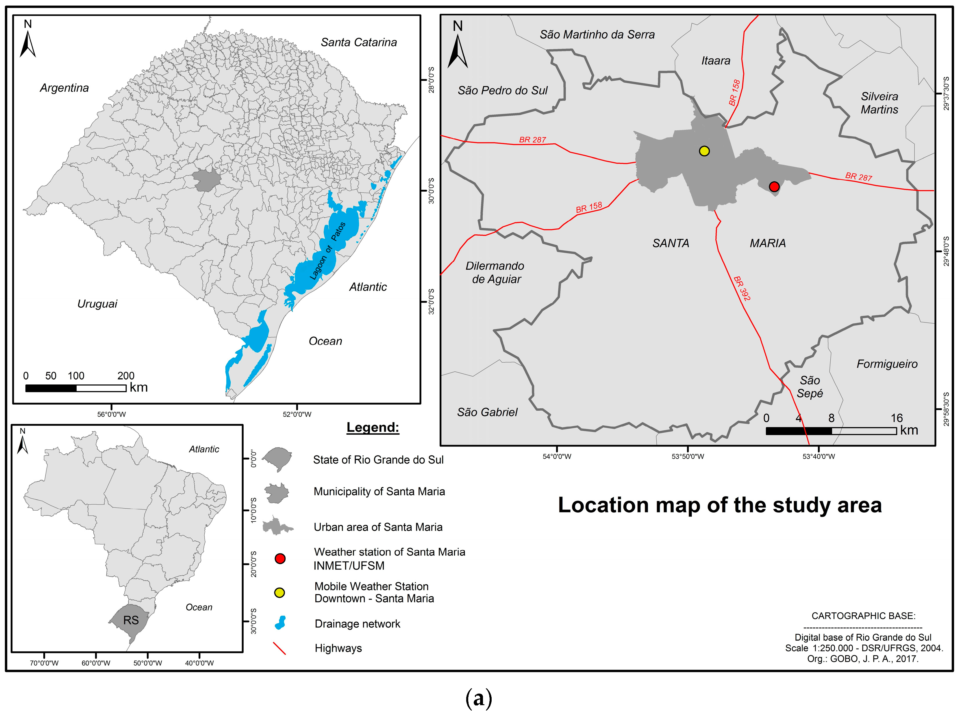
The meteorological and thermal sensation data were collected during 2015 and 2016 in the city of Santa Maria, Rio Grande do Sul, Brazil, which is located in the geographic center of the state and has an estimated population of 278,445 inhabitants [
46]. According to Köppen [
45], in terms of general climatic classification, the city is classified as type Cfa, with a hot and rainy temperate climate, no dry season, and a hot summer. The hottest month has a mean temperature higher than 22 °C and a mean air temperature in the hottest four months above 10 °C, and the coldest month has a mean temperature above 3 °C.
For this purpose, a Campbell CR100 Automatic Weather Station (AWS) was used, at a maximum height of 2.0 m, with a mobile aluminum tripod containing the following sensors (
Table 1):
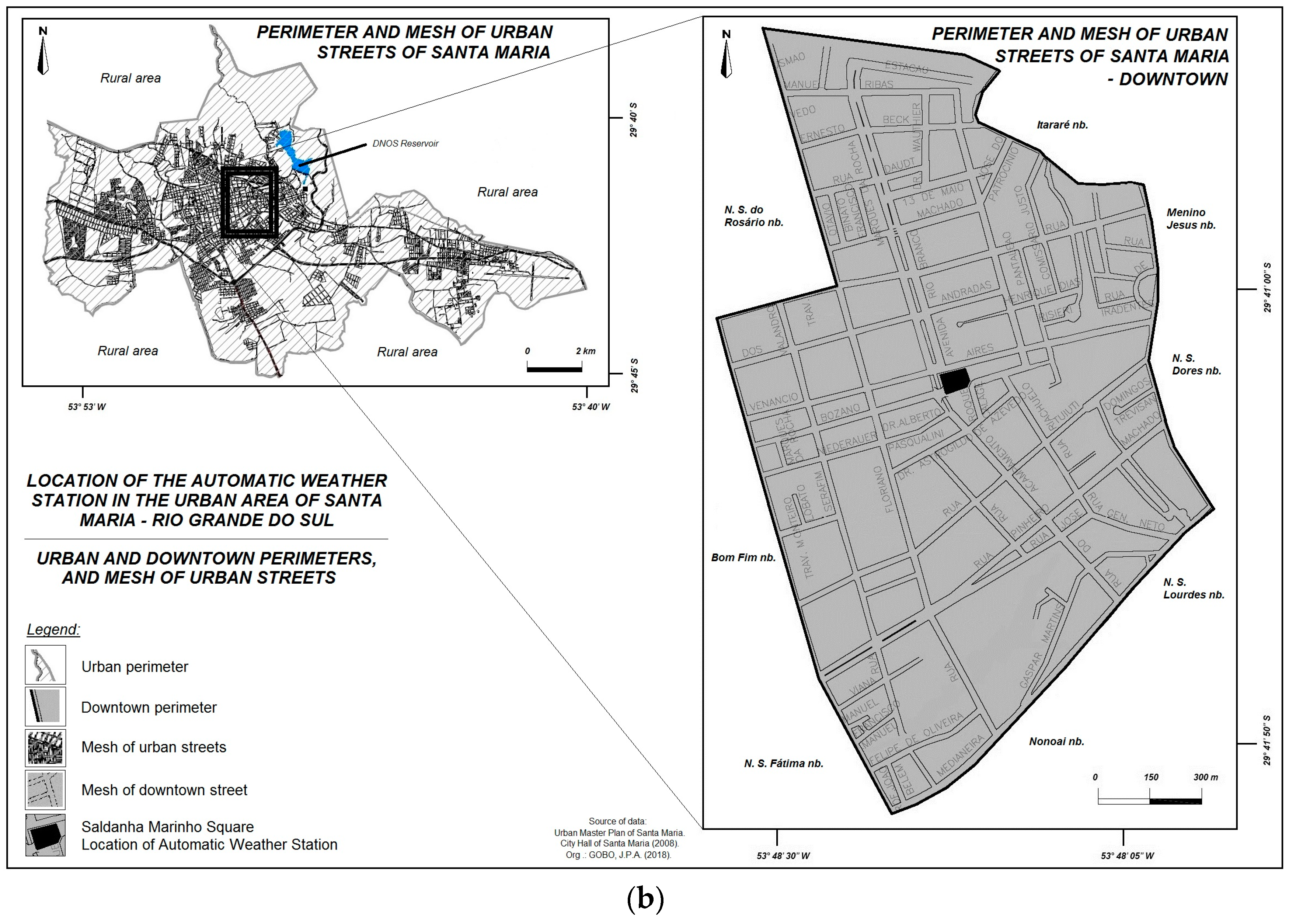
Primary data on air temperature, gray globe temperature—because the station was set up in an open space exposed to direct solar radiation [
47]—relative humidity, wind speed, wind gusts, global solar radiation, and rain were collected. The station was positioned in a paved area in the center of Santa Maria (
Figure 1).
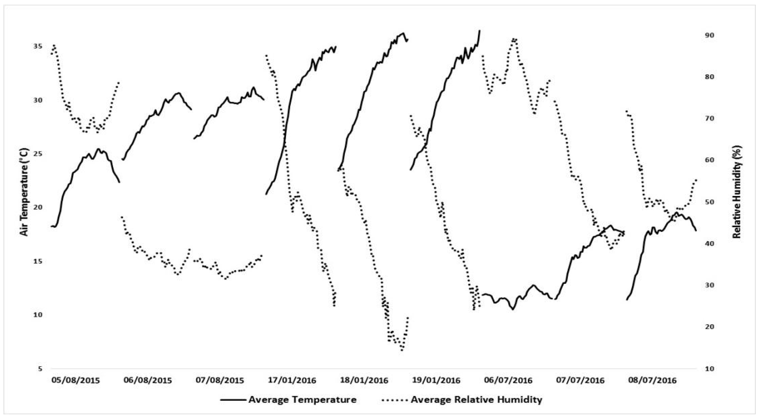
Field data collection was performed during the following periods: 5–7 August 2015, 17–19 January 2016, and 6–8 July 2016. These periods were selected as representative of summer (January 2016) and winter (July 2016). The period of August 2015 was used for the validation of the data.
The choice of the representative periods of summer and winter was aimed at demonstrating the seasonality of the data and evaluating its influence on the final results. The objective is to incorporate the region’s climatic amplitudes into the proposed models, because methodological and operational evaluations are not necessarily possible over the course of the entire year. The seasonal aspect is incorporated into the model to make observations in representative periods of summer and winter. Collection of meteorological data and interviews with the local population were performed from 9:00 a.m. to 5:00 p.m. local time during the field experiments described above. The model can also be applied to the night period, simply by including the input variables of this period. However, it is understood that the flow of people in this environmental profile is greater in the daytime and in the early hours of dusk.
On the days of field research, the 5–7 August 2015, period was characterized by a persistent high-pressure system anomaly (anticyclone positioned at approximately 30 degrees of latitude), with relatively slow displacement of high pressures, which persisted for several days. During the January 2016 field research days, it was possible to identify a pattern compatible with Santa Maria’s normal climatological averages for that month, which presented high temperatures with maxima above 32 °C. In the analysis of the next winter, during July 2016, above-average temperatures for Santa Maria were observed mainly in the first day of analysis, but after that day, temperatures were within the range expected for that season.
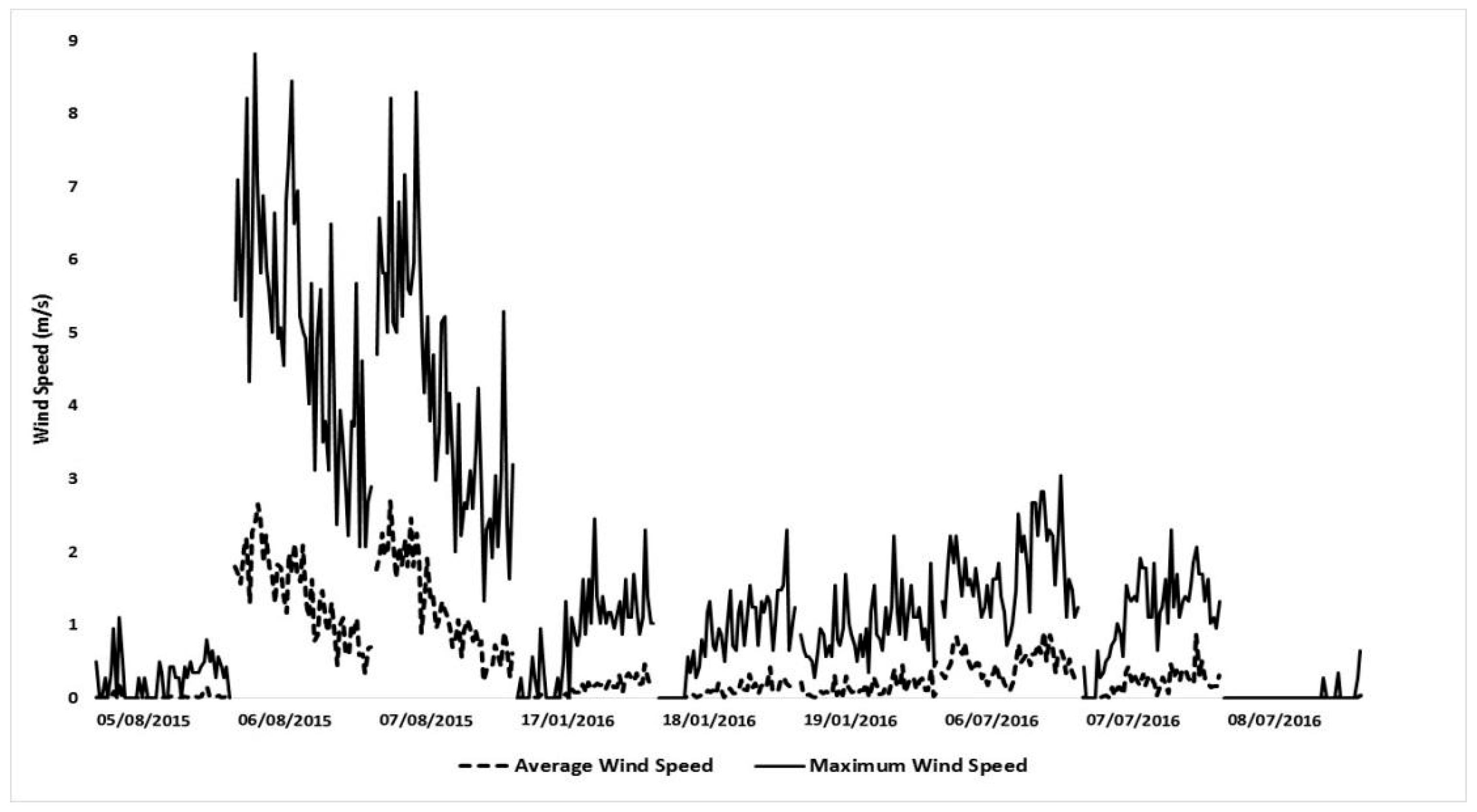
The mean temperature and relative humidity patterns observed in all periods of data collection are shown in
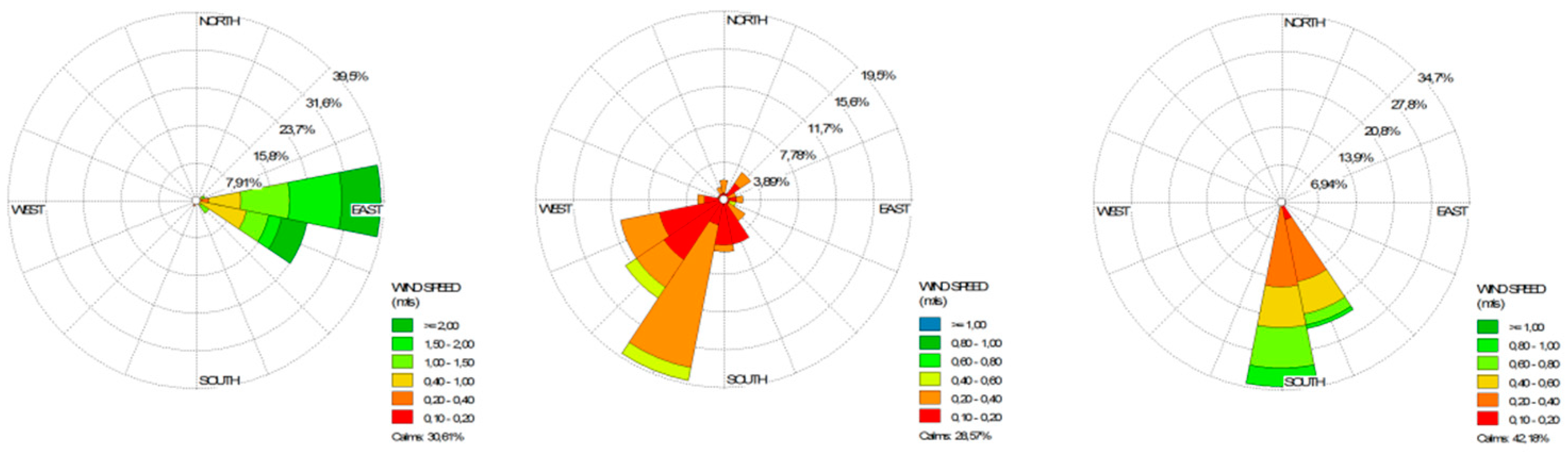
Figure 2. The patterns of average velocity and maximum wind speed are observed in
Figure 3 and the predominant direction of wind for the period of analysis is shown in
Figure 4.
The mean patterns of the main climatic attributes observed in the field are shown in
Table 2.
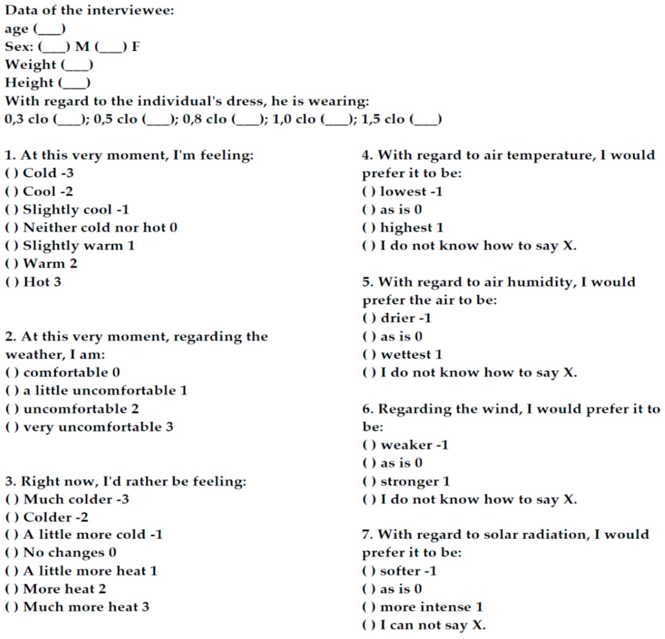
In the present study, only those individuals who had resided in the town for more than one year were interviewed to derive a function of the individual thermal history and environmental memory, as observed by Nikolopoulou et al. [
48], in a total of 1720 interviews (
Table 3). Interviewees also had to exhibit 0.3 to 1.5 clo of clothing insulation, which corresponds to wearing jeans and T-shirt or a suit [
49], and 300 W of physical activity, because only people in motion (walking) were included [
50]. The questionnaire used was an adaptation of the one included in the standard ISO 10551 (1995) (
Figure 5).
From the correlation between the environmental variables (air temperature, relative air humidity and wind speed) observed in the field and the subjective answers, a new empirical index was proposed. Only the data referring to the collection days in January and July 2016 were used because the August 2015 data were later used to validate the results of the index by means of an uncertainty test for the samples and a Student’s t-test.
All statistical procedures were performed using the statistical software R, and the multiple linear regression method is described by the following mathematical expression:
where
n is the number of terms in the equation, α
n are the parameters (constants) obtained by the regression,
c is the constant that corresponds to the point where the adjusted line intersects the y-axis
, Y is the dependent variable, and x
n are the independent variables.
In the present study, what we call the mean index is, in fact, the mean of the responses observed in the field for a given climatic variable value. Since
Y is a random discrete variable whose possible values are finite, the best way to estimate the expected mean index value in a given time interval is to use the formula of the expected value for discrete random variables, or a finite case, since the responses are limited to the [
32] 7-point class interval:
where
yk is the possible value, and
pk is its respective probability in some independent tests.
In the case of the present study,
where
Ik is the mean index, and
pk is the probability estimated by dividing the number of responses to the index by the total number of interviews performed in a given interval.
Subsequently, more than 100 regressions were performed with multiple variables to obtain the appropriate parameters for the various situations examined. Regressions were also tested using absolute humidity rather than relative humidity. This is because collinearity was observed in the results, and the variance inflation factor (VIF) test was used, which, according to Marquardt and Marquardt and Snee [
51,
52], is used to determine the variables with VIF values exceeding 10, which should be excluded to prevent compromising the model.
Finally, the index was validated with the data obtained in the first field survey conducted in August 2015, and through the uncertainty test for the samples,
where
σi is the uncertainty of the mean of the votes obtained through interviews,
yk is the
k index (
k = −3 to 3), and
pk is the estimated probability of obtaining the
yk index.
After the uncertainty calculation, the
t-test or Student’s test was performed as given by the following equation:
where
Imean is the comfort index obtained by the mean of the votes obtained in the interviews,
Imodel is the index calculated by the model,
σ is the uncertainty of the mean of the votes obtained through interviews, and
n is the number of samples (number of interviews to obtain the calculated mean).
The multiple linear regression method is simple and robust, since the linearity assumptions of the data, such as normality (obtained by the measure of obliquity and kurtosis of the distribution) were verified, which were, finally, executed in the process method validation [
53].
In order to obtain an even more efficient validation for the developed model, 33% of the data were used for the comparison between this and the already traditional models in the literature, including Physiologically Equivalent Temperature (PET) [
54], Standard Effective Temperature (SET) *, and Predicted Mean Vote (PMV) [
30], which had their classes adjusted by Gobo, Galvani and Wollmann [
55] for the same climatic situation in Santa Maria.
3. Results
We chose to develop a simplified thermal comfort index for winter and summer conditions based on the independent variables including air temperature, relative air humidity, and wind speed. These variables are easily measurable and available in databases from meteorological institutes.
The assumptions of the linear models, as if the predictors are normally distributed and have equal variances, are verified by Asymmetry, Curtosis, and Heteroscedasticity measurements obtained by the GVLMA (Global Validation of Linear Model Assumption) package of the R programming language (
Table 4).
The correlation between logistic and linear regression models was ±98%, proving unnecessary the use of two different methods, and therefore, the multiple linear regression model was used. The values of
Table 3 show acceptable results, which increase the confidence in the model.
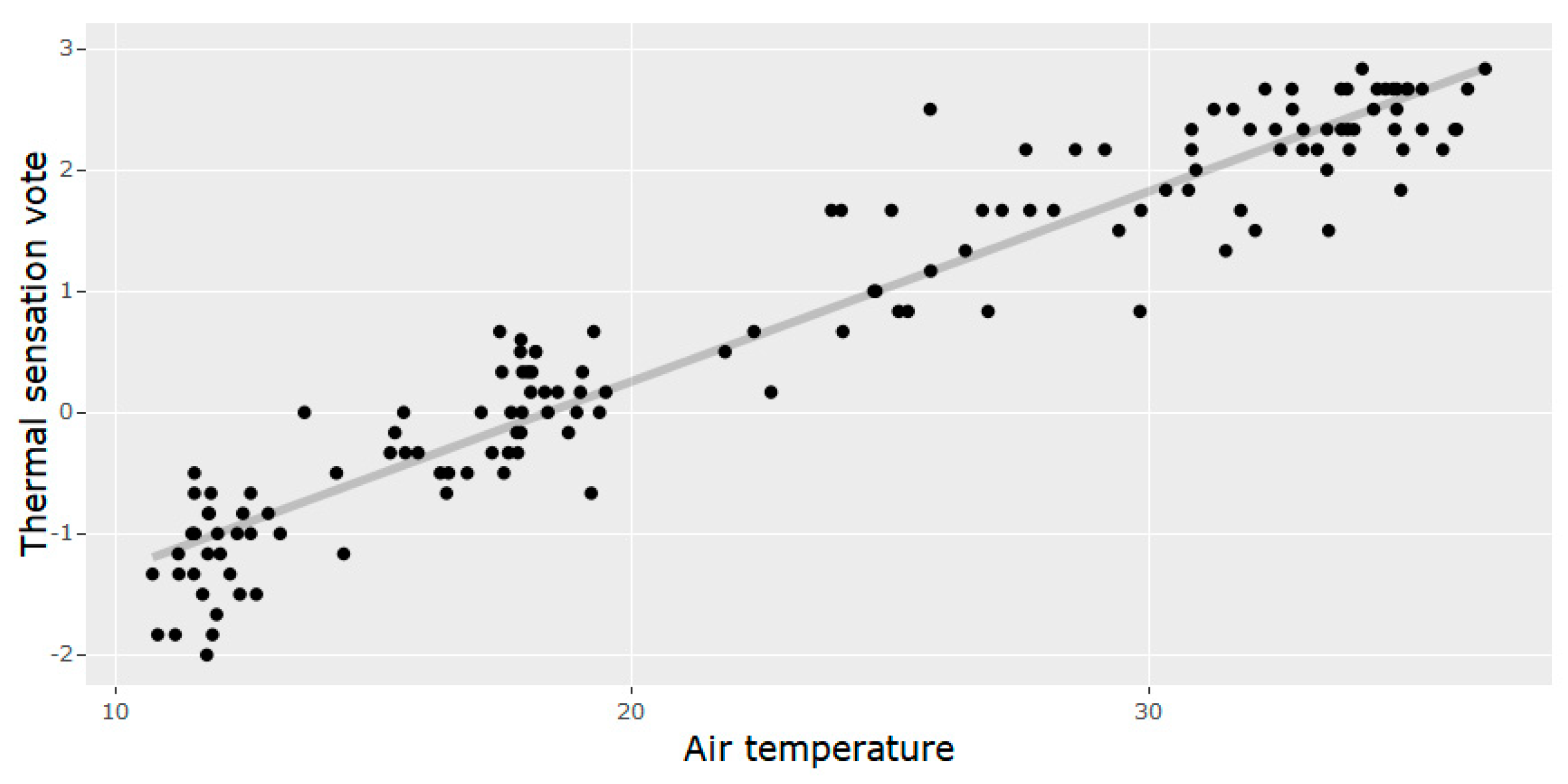
The results revealed a strong positive correlation between the means of the thermal sensation votes and air temperature, with an R
2 value equal to 0.96 (
Figure 6).
The correlation analysis of air temperature with the other variables indicated a strong negative correlation with relative air humidity for both July and January. However, the strong correlation between the variables air temperature and relative air humidity may impair the model results due to internal collinearity.
According to Monteiro et al. [
56], when the relative air humidity has a significant negative correlation with air temperature, direct consideration of this information may lead to the false interpretation that higher relative humidity leads to more intense cold sensations. However, relative humidity has a strong negative correlation with air temperature, approaching 1 in the most restricted data set observed by the author. Taking into account the fact that the absolute humidity is more or less constant during a given period, higher air temperature results in lower relative humidity. Thus, the correlation obtained for air humidity is largely due to the variation in air temperature [
56].
Monteiro et al. [
56] add that when considering a larger data set that includes hotter and colder thermal conditions, a longer series of days will have different absolute humidities, leading to different correlations between air temperature and relative humidity. Nevertheless, relative humidity is dependent on air temperature, and therefore, as is observed in the subsequent analyses, it is necessary to consider the absolute humidity for effective testing of the effects of humidity on the subjective thermal sensation responses.
Thus, a new regression was performed for the same parameters, but with the variable absolute humidity (
g of water vapor per m
3 of air) replacing relative humidity. However, the results obtained for the absolute humidity variable did not show a considerable statistical improvement, as shown in
Table 5, where the significance value of the variable absolute humidity decreased relative to relative humidity, becoming 0.395 (
Table 5) compared to the significance level of 0.711 for relative humidity (
Table 6).
Thus, the VIF was calculated for the previously selected variables. As stated by Marquardt [
52], variables with VIF values greater than 10 should be excluded; however, the collinear variables do not add any relevant value to the model (
Table 5), and values above the threshold established by Marquardt [
52] were not observed, so it was decided to keep relative humidity in the construction of the index.
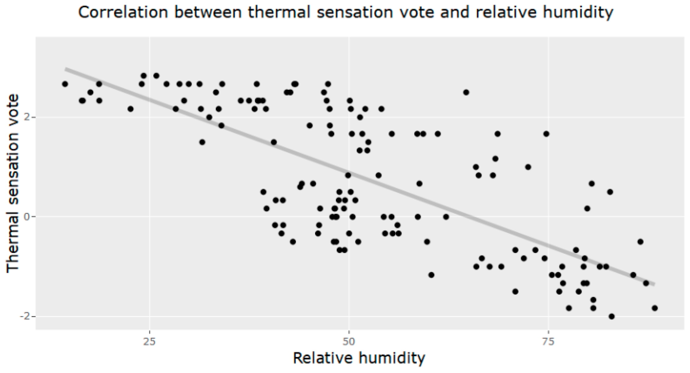
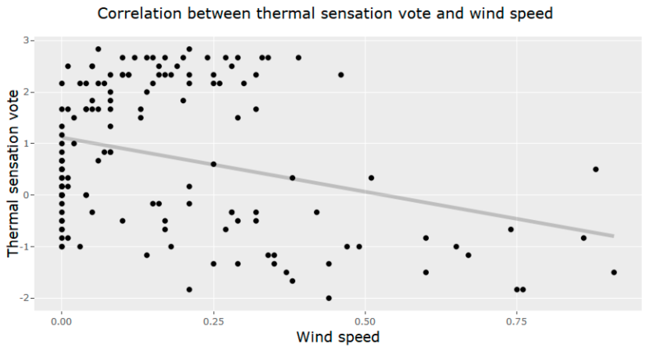
The relative air humidity and the means of thermal sensation votes showed a strong negative correlation, with an R
2 value of 0.736 (
Figure 7). However, the relative humidity had a weak positive correlation with wind speed, with an R
2 value of 0.209. Wind speed had a weak correlation with all the other variables, with the correlation between wind and mean thermal sensation votes being negative, which was also the case between wind speed and air temperature (
Figure 8).
The probability density function (PDF)—or density of a continuous random variable—was calculated for the means of the thermal sensation votes of the individuals interviewed during the entire study (winter and summer) as well as for mean air temperature, mean relative humidity and mean wind speed for that period. The PDF is a function that describes the relative probability of these random variables when taking a given value.
Table 5 shows the results of the linear regressions performed for the mean values reached for the conditions surveyed during the study (summer and winter) to obtain the model.
Thus, the model had high multiple R2 and adjusted R2 values of 0.926 and 0.924, respectively, whereas the statistical test F showed a high value of 584.9, which confirms that together the variables contribute to the prediction of the independent variable.
Next, an equation was defined that considers the three independent variables (Tair, RH and S) correlated for the situation survey and the mean value of perceived thermal sensation in each (based on the results of the questionnaires applied in January and July 2016):
where
BSI = Brazilian Subtropical Index,
Tair = air temperature (°C),
RH = relative humidity (%), and
S = wind speed (m/s).
The Brazilian Subtropical Index (BSI) is the proposed model, which is defined as a thermal sensation scale based on the mean vote of individuals interviewed during winter and summer using the 7-point scale (
Table 7).
Validation of the Proposed Empirical Index
The model was validated using a Student’s t-test to evaluate the relationship between the comfort index predicted by the BSI model (obtained with data from January and July) and the thermal sensation votes of the interviewees. For this purpose, 857 interviews were obtained from the August 2015 survey and compared to the BSI results for the same period.
The hit rate obtained via the validation of the index is 88% for the first test, 81% for the second test and 79% for the third test. These values are higher than those observed by Gobo et al. [
54] in a study calibrating the interpretative ranges of PET, SET and PMV indices for Santa Maria, where the authors identified hit rates after the calibration of 69.3% for the PET, 64.9% for the SET and 58.7% for the PMV index.
As observed in the study of Salata et al. [
36], the Mediterranean Outdoor Comfort Index (MOCI) presented an adjusted R
2 value of 0.395, an R
2 value of 0.398, and a Pearson coefficient of 0.631, whereas the BSI presented an R
2 value of 0.926 and an adjusted R
2 value of 0.924 and a higher Pearson coefficient, 0.790.
Comparing the results obtained during the development and validation of the BSI with those observed by Ruiz and Correa [
8], the adjusted R
2 value of the latter is closer (0.719), with a predictive capacity of 73%, which is very close to that observed in the validation of the BSI.
When comparing the results of the Global Outdoor Comfort Index (GOCI) developed by Golasi et al. [
10], an adjusted R
2 value of 0.379 and a Pearson coefficient of 0.616 were observed for the GOCI, whereas the BSI presented an adjusted R
2 value of 0.924 and Pearson coefficient higher than 0.790, further indicating the efficiency of the BSI.
The BSI hit rates are higher than 50%, and it should be noted that Nikolopoulou and Steemers [
57], when analyzing psychological aspects related to thermal sensation, found that climatic variables have a strong influence on thermal sensation, but these explain approximately 50% of the variation between objective and subjective assessments of comfort.
Of the approximately 165 thermal indices developed to date, only 4 (PET, PMV, Universal Thermal Climate Index (UTCI) and SET *) are widely used in studies of outdoor thermal perception [
58]. Thus, a correlation test was performed between the respondents’ thermal preference responses in the period used for the BSI validation (August 2015) and the PET, SET * and PMV models calibrated by Gobo, Galvani and Wollmann [
54] to Santa Maria. The results are described in
Table 9.
It is important to note that the correlations made between the PET, SET *, PMV, and the thermal preference responses of the interviewees (
Table 9) were only for the BSI validation period of August 2015, differing from the period used by Gobo, Galvani and Wollman [
55] in the calibration of the mentioned models, where the whole series of August of 2015, January and July of 2016 was used.
The low efficiency of the PET, SET * and PMV indices for the analyzed period can be explained in part by the large size of the comfort range of these indices as calibrated by Gobo, Galvani and Wollman [
54] for the study area, featuring 16 °C–24 °C for PET, 17 °C–23 °C for the SET and –1–0.8 for the PMV. Potchter et al. [
58], when analyzing a work done with PET in the Cfa climate [
45], signals for the acceptance of the comfort range of 87% of the case studies between 24 °C and 27 °C and up to 94% of the cases between 25 °C–26 °C, which considerably limits the comfort range for these indexes. Therefore, the validation of the BSI presented greater efficiency when compared to the other indexes commonly used in studies appearing in the literature.
4. Conclusions
The index obtained by means of multiple linear regressions presented high statistic values that did not reveal any anomalous behaviors that indicated inadequacy of the chosen model. The multiple linear regression model presented considerable results when compared to the other regression models, which increased confidence in the use of this model. The VIF demonstrated that the collinear variables do not add any relevant value to the model, with no values above the limit established by Marquardt [
52] being found.
The proposal of the Brazilian Subtropical Index (BSI) provides a simple and easy-to-apply model with temperature, relative air humidity, and wind velocity as input variables. Therefore, it accounts for meteorological attributes commonly measurable in conventional and automatic surface meteorological stations.
The results expressed the perception of the interviewees regarding comfort and thermal discomfort for the locality of Santa Maria, a subtropical climate region in southern Brazil. A high rate of model accuracy, with a multiple R2 and adjusted R2 of 0.926 and 0.924 respectively, and a high statistical F with value of 584.9, confirmed that, together, the modeled variables contributed to the prediction of the independent variable.
Thus, like any statistical model, the index proposed here has limitations, and its effectiveness in situations different from those analyzed should be explored based on more detailed studies and with a longer observation times.
Finally, BSI validation has proved to be effective. With hit rates higher than 80%, these values are higher than those observed for the PET, SET and PMV indices for Santa Maria, which indicates the efficiency and reliability of the model.

 ,
, 


