1. Introduction
Haze is an important environmental issue worldwide and has received increasing attention due to its impacts on visibility, air quality, radiative forcing, regional climate, and human health. Aerosols affect Earth’s radiation balance directly by scattering and absorbing solar shortwave and longwave radiation. They also act as condensation nuclei for clouds, thereby changing the clouds’ microphysical properties and life cycles, and thus affect the climate system indirectly [
1,
2]. Additionally, the World Health Organization has indicated that aerosols (especially fine particles) can produce adverse effects on human health [
2]. The China Meteorological Administration (CMA) defines haze as a condition in which atmospheric visibility is less than 10 km and relative humidity is less than 90% [
1]. China’s rapid economic growth, urbanization, population expansion, and increased industrial activity have led to increasing amounts of particles being discharged into the environment, resulting in frequent air pollution events [
3].
Because of the advantages of short wavelength, light can interact better with small particulates than can microwaves, and optical instruments, such as Lidar and optical particulate counters, are often used to observe the properties of haze. Huang
et al. statistically analyzed the monthly and quarterly variations in aerosol extinction coefficients over Shanghai using Micropulse Lidar (MPL) data from July 2008 to January 2009 [
4]. The results showed that most of the aerosol was concentrated in the layer below 3 km and that the optical extinction coefficient in the layer below 2 km contributed 84.25% of that below 6 km [
4]. Haze events in Shanghai were analyzed by Pan
et al. Their analysis showed that severe haze events in Shanghai often occurred under conditions of calm wind and weak radiation. The humidity had an important impact on visibility during the severe haze events, and the altitude variation of the Planetary Boundary Layer (PBL) determined the intensity of the haze [
5]. Additionally, Zhang used spaceborne and ground-based Lidar observations over the Jinhua Basin in the province of Zhejiang to analyze the aerosol vertical distribution during a haze event both temporally and spatially [
6].
The laser ceilometer is a simple elastic scattering lidar system in which a small power laser is used. Compared with common lidars, the ceilometer often has a low signal-to-noise ratio (SNR) that is about 1200 in clear air. However, for the increased atmospheric particulates during a haze episode, the ceilometer can obtain a sufficient signal-to-noise ratio to invert the optical properties of the particulates. The SNR at an altitude of 500 m during the hazy episode in this article is about 4000. The most important advantage of a ceilometer, as a simple lidar system, is that it can function in harsh circumstances and poor weather conditions under which other types of lidar are often invalid. Furthermore, according to its schedule, CMA will soon construct a ceilometer network for cloud observation. If information about haze could be retrieved from the ceilometer network in addition to that of cloud, it would benefit the monitoring of haze around China and permit full use of the ceilometer network data. In previous research, we demonstrated the feasibility of aerosol detection during fog-haze processes using a ceilometer [
7]. In this study, based on data from two ceilometers with two different wavelengths, more microphysical particulate characteristics of a haze were studied intensively.
2. Facilities and Method of Analysis
In principle, a ceilometer is a simple lidar system. For the design purpose of detection of cloud base height, which often has a large backscatter coefficient, the ceilometer often has a more simple structure than common lidar. As the laser pulse is emitted by the lidar system flying in the atmosphere, the laser pulse is scattered by aerosol, molecular components, or cloud. The partial scattered signal is sensed by the high gain detector (usually a PMT) and digitalized by a photon counter. Optical properties such as the backscatter coefficient and the extinction coefficient can be retrieved from the intensity of the backscattered signal; thus, cloud distribution information can be obtained.
In this study, two ceilometers were used. One was the MPL-4B, with a laser wavelength of 532 nm. Other detail specifications of this system can be found in various sources and are not listed here [
8]. The capability of the MPL-4B has been verified through aerosol and cloud projects, such as the Micro-Pulse Lidar Network (MPLNET) and Atmospheric Radiation Measurement (ARM) projects [
9]. The other ceilometer used was the Vaisala CL31, which uses a 910 nm diode with a pulse frequency of 6.5 kHz as an optical source. The lens is divided into transmitting and receiving areas. The middle of the lens focuses the outgoing laser beam, and the outer part of the lens collimates the backscattered light onto the receiver. Because the beam is transmitted coaxially with the receiver field of view, the system provides robustness against changes in mechanical alignment. The CL31 has a shield with a blower and a heater, which enable reliable operation in precipitation and in extreme temperatures. The CL31 provides an aerosol signal profile as well as the height of the cloud base. Although in most cases the backscatter signal of aerosol is too weak to retrieve extinction, the optical properties of haze can be obtain by using the Klett method [
7]. And the overlap correction before the data inversion had carried on. So, above the first bin (blind range: the lowest 30 m), the ceilometers’ data can be used to analyze the properties of aerosol. The main parameters of the two ceilometers are shown in
Table 1.
Table 1.
Parameters of the CL31 and MPL-4B.
Table 1.
Parameters of the CL31 and MPL-4B.
| | CL31 | MPL-4B |
|---|
| Laser | 910 nm | 532 nm |
| Measurement range | 7.7 km | 10 km |
| Reporting resolution | 5/10 m | 15/30/75 m |
| Measurement interval | 2…120 s | 1 s…900 s |
| Pulse frequency | 6.5 kHz | 2.5 kHz |
| Input power | 100/115/230 V | 100/240 V |
| Power consumption | 310 W | 350 W |
| Dimensions | Total: 1190 × 335 × 324 mm
Measurement unit: 620 × 235 × 200 mm | 380 × 305 × 480 mm |
| Weight | Total: 32 kg Measurement unit: 13 kg | 16 kg |
The Grimm 180 is a field measurement instrument based on the principle of light scattering. The pump inputs an ambient air sample including particles into a gas chamber at a constant rate of flow. The laser irradiation is scattered by the particulates in the air flow and then sensed by the detectors. The received pulse signal frequency and intensity are then related to the number and diameter of the particles. The Grimm 180 is an online environmental particulate matter monitor that can simultaneously measure PM
10, PM
2.5, and PM
1 in the environment. The particle size range of measurement is 0.25 um to 32 um (31 channels), and the measurement range of mass concentration is 0.1 to 6000 μg/m
3 [
10].
To select a tool for routine observation of cloud base height during meteorological operations, campaign observation of cloud using several kinds instruments, including ceilometers, was organized by the CMA at the Nanjiao Surface Meteorological Station from June to October 2014. During the observation, the CL31 was a candidate tool for cloud observation. It showed notable capability and stability during the entire observation. The MPL-4B was installed in an air-conditioned room with a window in the ceiling to emit and collect backscattered light. The capability of the MPL has been demonstrated in other projects. Here, it functioned as the standard tool to evaluate the candidate tools. The distance between the MPL-4B and the CL31 was set as 3 m to ensure that the two instruments would detect the same cloud or aerosol in the same atmospheric column. Routine observation results of meteorological elements from the Nanjiao surface station were also collected to analyze the haze process. The Grimm system was mounted at Chaoyang Meteorological Station, another surface station that is about 10 miles from the Nanjiao surface station. For the scale of the haze phenomenon, the work assumed that all of the instruments detected the same sample in the haze. In the haze situation, the Klett method was used to retrieve the extinction coefficient profiles of the pollutants according to the following formula [
11]:
in which K is related to the wavelength of the laser radar and the properties of the aerosol, and the range is 0.67–1.
Sm =
S(
Zm), σ
m = σ(
Zm), and
Zm is the greatest measurement range. Using the Klett method, extinction coefficients can be inverted from the MPL-4B and the CL31. Based on the extinction coefficients at different wavelengths, the microphysical evolution of the haze was analyzed by combining data with the size spectrum from the Grimm.
3. Observed Characteristics
In this study, two ceilometers with different wavelength were used to observe a haze episode that occurred on 2 October 2014. A weather condition analysis showed that high-altitude vertical wind shear and long-distance transport of particles were the main reason for the formation of the haze. During the haze process, the upper airflow was mainly from the area of Inner Mongolia, while the low-level airflow was mainly from the northeast, with variation in direction ranging from northeast to southeast. Pollutants from Hebei Province were transported to the city of Beijing. With relatively stable weather parameters in Beijing, both the transported pollutants and the pollutants generated by the mega-city contributed to the main part of the haze process.
3.1. Surface Meteorological Elements
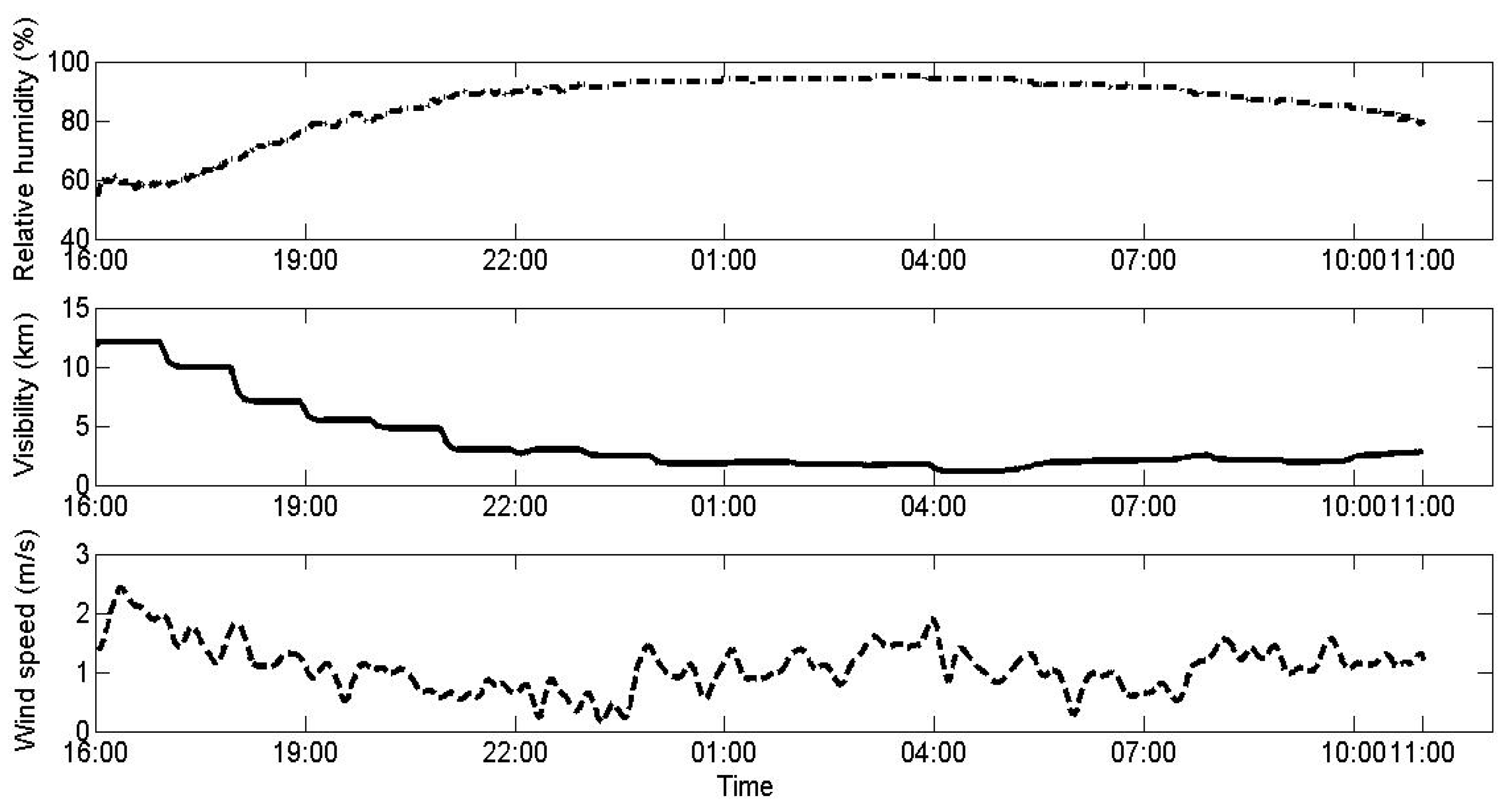
Figure 1 presents the surface meteorological elements during the haze from 16:00 on 2 October to 11:00 on 3 October 2014. The variations of relative humidity, visibility, and wind velocity are provided in the figure, respectively. The figure shows that the wind velocity remained as small as 1 m/s in the time segment from 16:00 to 01:00. The low wind velocity inhibited diffusion of the pollutants, as reported by Pan
et al. [
5]. As pollutants accumulate, absorption of moisture by nuclei leads to further deterioration of visibility. As shown in
Figure 1, in this time segment, the relative humidity increased from 55% to 93% while the visibility decreased from 12 km to 1.8 km. According to the definition of haze that was stated previously, haze began at 17:00 when the visibility was less than 10 km and the relative humidity was 60%.
Figure 1.
Evolution of relative humidity, visibility, and wind velocity during the haze episode.
Figure 1.
Evolution of relative humidity, visibility, and wind velocity during the haze episode.
3.2. Analysis of Aerosol Optical Properties
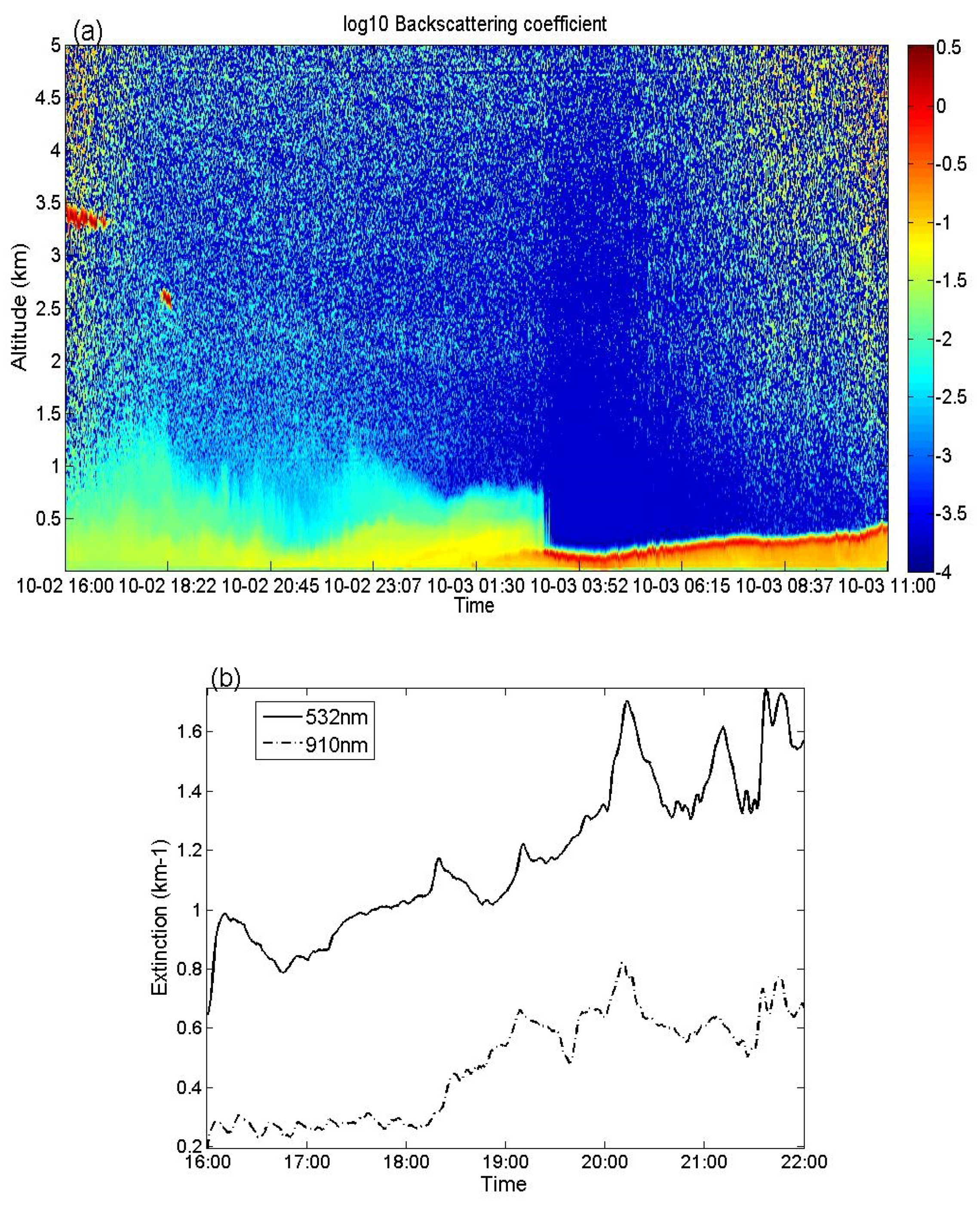
Figure 2 presents the variations of the extinction coefficient inverted from the CL31. The slope method is used to retrieve the boundary layer height from the extinction profiles of aerosol. It is clear that the boundary layer becomes progressively lower after 18:00 on 2 October. Due to the existence of this boundary layer, the pollutants could not diffuse and accumulated in the lower atmosphere. As shown in
Figure 2a, the color indicating the magnitude of the extinction coefficient becomes greater, especially in the altitude range below 0.5 km. During the night of 2 October, radiation inversion restricted pollutant diffusion in the vertical direction. Pollutants concentrated at the top of the boundary layer until the haze dissipated. Before 22:00, the relative humidity increase from 55% to 90%, and the extinction coefficient at 532 nm increased from 0.65 km
−1 to 1.84 km
−1 while the extinction coefficient at 910 nm increased from 0.2 km
−1 to 0.8 km
−1, at the height of 90 m, as shown in
Figure 2b.
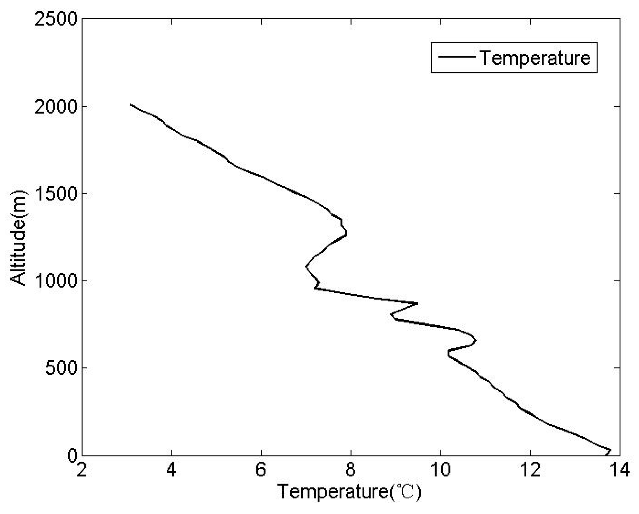
Figure 3 is a radiosonde temperature profile acquired at 08:00 on 3 October, the vertical resolution is 30 m. It shows an obvious temperature inversion at the height of 500 m, which is consistent with the height of the boundary layer in
Figure 2a at around 08:00 on 3 October. At this time, affected by the inversion layer, the atmosphere tended to be stable, and convection could not occur easily. Because of the low wind speed and the inversion phenomenon caused by temperature, the aerosol particles near the ground could not diffuse, and the accumulation of the aerosol particles promoted the emergence of the haze.
Figure 2.
Sequence diagram of backscattering (a) and diurnal change of extinction coefficients (b).
Figure 2.
Sequence diagram of backscattering (a) and diurnal change of extinction coefficients (b).
Figure 3.
Radiosonde temperature profile at 08:00 on 3 October 2014.
Figure 3.
Radiosonde temperature profile at 08:00 on 3 October 2014.
3.3. Properties of Hygroscopic Growth
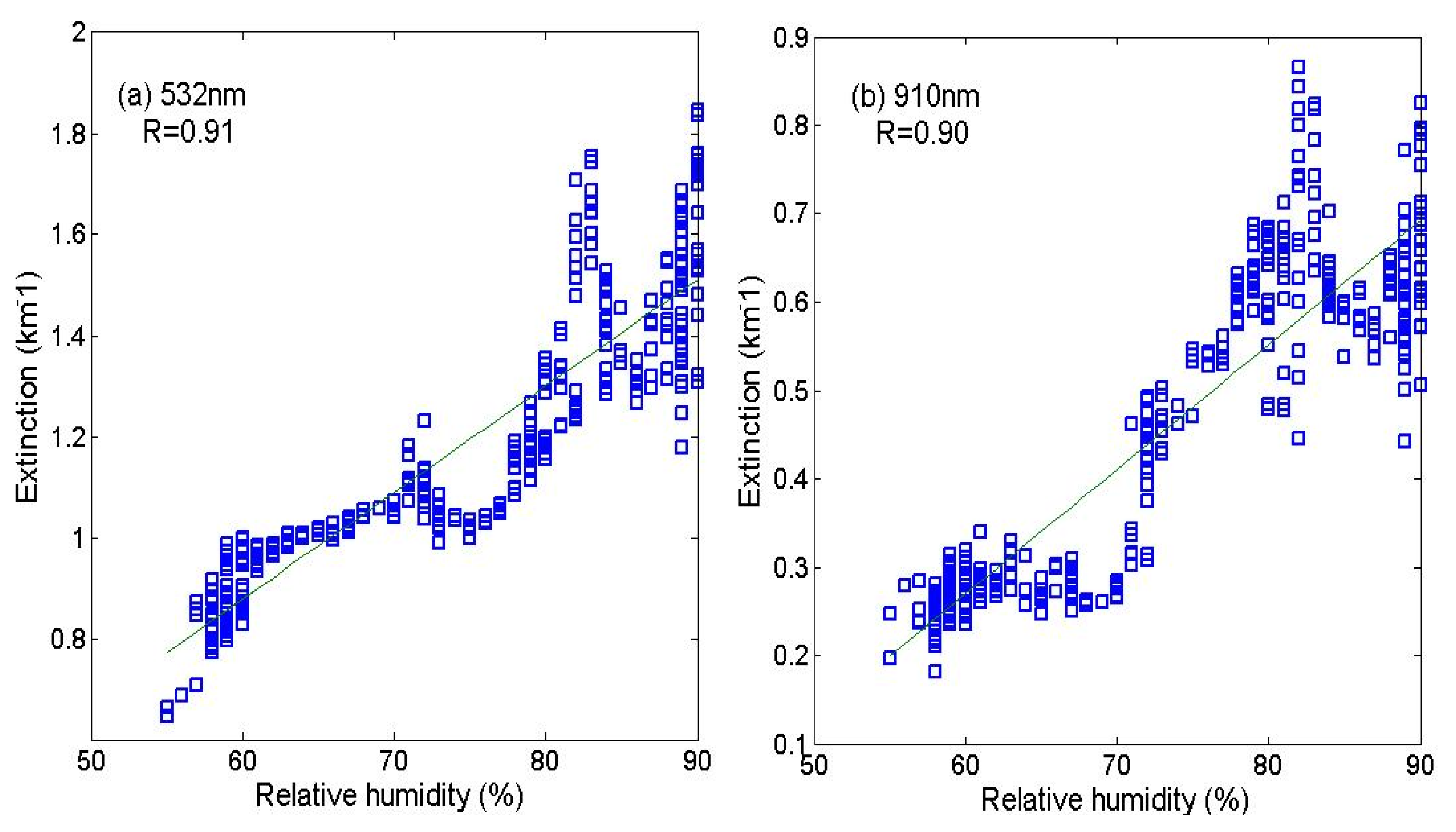
The relationships between the relative humidity and the extinction are shown in
Figure 4. The squares are measurement data, and the lines are the fitting results. A strong positive correlation between relative humidity and extinction coefficient is apparent at both laser wavelengths (532 nm and 910 nm). The correlation coefficients between relative humidity and extinction coefficient are 0.91 at wavelength of 532 nm and 0.9 at wavelength of 910 nm. The positive correlations indicate that the extinction coefficients increased simultaneously with the growth of aerosols caused by moisture absorption. The aerosol particles had dominantly hydrophilic compositions and strong ability to absorb moisture, which was ideal for an analysis of the characteristic of moisture absorption. When the relative humidity reached 70%, the extinction coefficient and the relative humidity showed a negative correlation, mainly because of an increase of wind speed at this time. As there was a decrease of scattered signal from surface particles, the extinction coefficient decreased correspondingly. However, with the continued increase of relative humidity, the solid-liquid surface chemical reaction caused the aerosol extinction coefficient to increase significantly, which means that the haze had entered the stage of hygroscopic growth [
12].
The hygroscopic growth factor (GF) of a particle is defined as the quotient between a particle’s extinction coefficient at a given relative humidity (RH) and its extinction coefficient at a (typically lower) reference humidity (RH0) [
13,
14]. According to this definition, GF can be written as
in which σ(
RH) is the extinction coefficient at a given relative humidity and σ(
RH0) is the extinction coefficient at a given reference relative humidity. For the case of this haze, a relative humidity of 55% was selected as the reference relative humidity [
15].
Figure 4.
Comparison between relative humidity and extinction coefficient for (a) 532 nm and (b) 910 nm.
Figure 4.
Comparison between relative humidity and extinction coefficient for (a) 532 nm and (b) 910 nm.
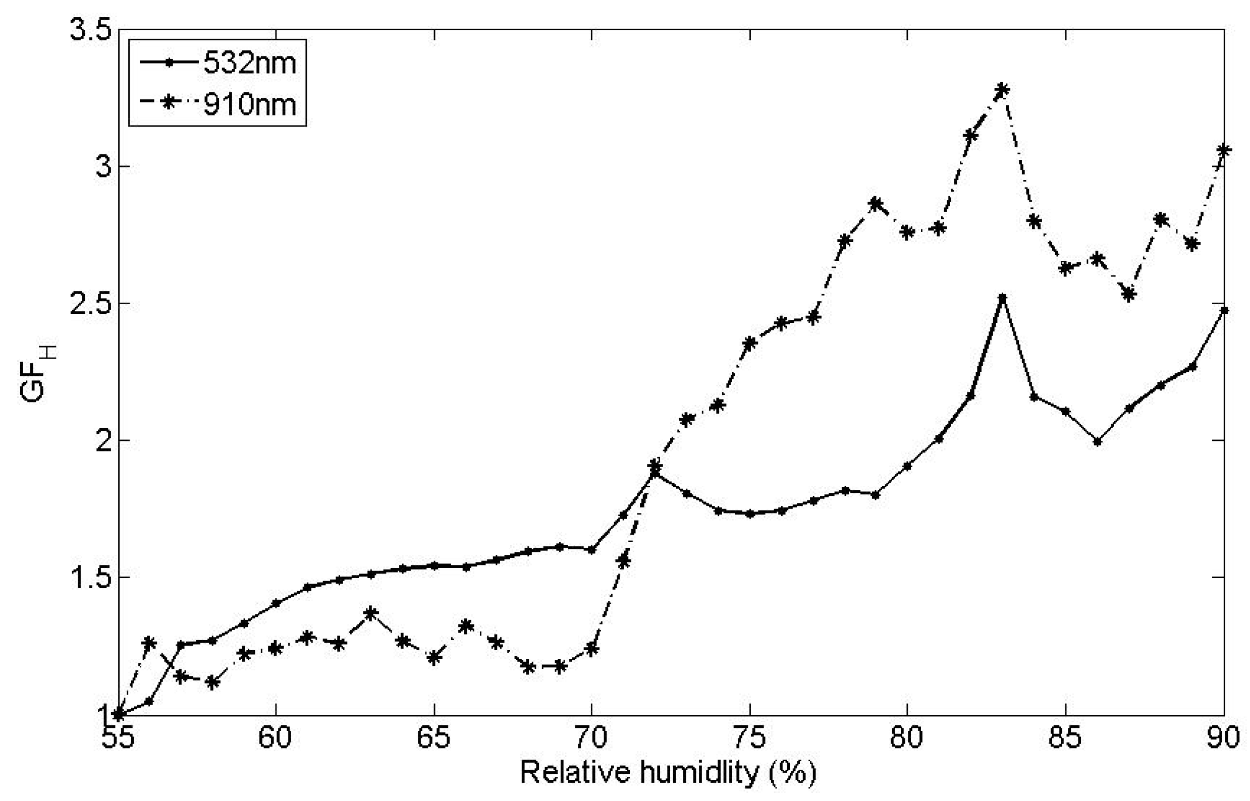
The hygroscopic growth factors at different values of relative humidity are presented in
Figure 5. From the figure, although the hygroscopic growth factors increase with increasing relative humidity, the detailed variations at the different wavelengths are not identical. Before the relative humidity of 70%, the hygroscopic growth factor increases slowly. The growth was relatively slow in this time segment because the size of the pollutants was small and both wavelengths were relatively longer than the size of the pollutants. In this case, scattering is much less sensitive to growth of the pollutants, especially for the relatively long laser wavelength of 910 nm. The hygroscopic growth factors at 532 nm and 910 nm are 1.88 and 1.89, respectively, which is consistent with the results provided by Liu [
16]. After the relative humidity of 72%, the hygroscopic growth factor for the 910 nm wavelength increased rapidly and become larger than that of the 532 nm wavelength. The reason for this change is that, as the pollutants became larger, the longer wavelength became more sensitive to them than the shorter wavelength [
17]. The hygroscopic growth efficiency of the particles’ extinction coefficient is described by the normalized hygroscopic growth factor GF’. Generally, the definition of GF’ is the hygroscopic growth factor GF divided by the change of relative humidity [
16]. From the normalized hygroscopic growth factor GF’ that was calculated as the relative humidity increased from 73% to 90%, the hygroscopic growth efficiency at 910 nm and 532 nm was 16.35 and 9.55, respectively. The normalized hygroscopic growth factor GF’ of the two wavelengths showed that the GF’ at the wavelength of 910 nm was almost two times larger than that at the wavelength of 532 nm. The difference between the GF’ values shows that the 910 nm wavelength becomes more sensitive as particle size increases.
Figure 5.
Change of hygroscopic growth factors with relative humidity.
Figure 5.
Change of hygroscopic growth factors with relative humidity.
3.4. Relationship between the Hygroscopic Growth Factors and Angstrom Exponent
With the assumption of the Junge size distribution, the aerosol scattering Angstrom exponent (AE) reveals aerosol size information according to Mie theory. AE has an adverse relationship with variation of the size distribution of the aerosol, such that the larger the size of the aerosol, the smaller the AE. Based on two ceilometers used.
In this study, AE can be derived from the extinction coefficients at 532 nm and 910 nm using the following formula:
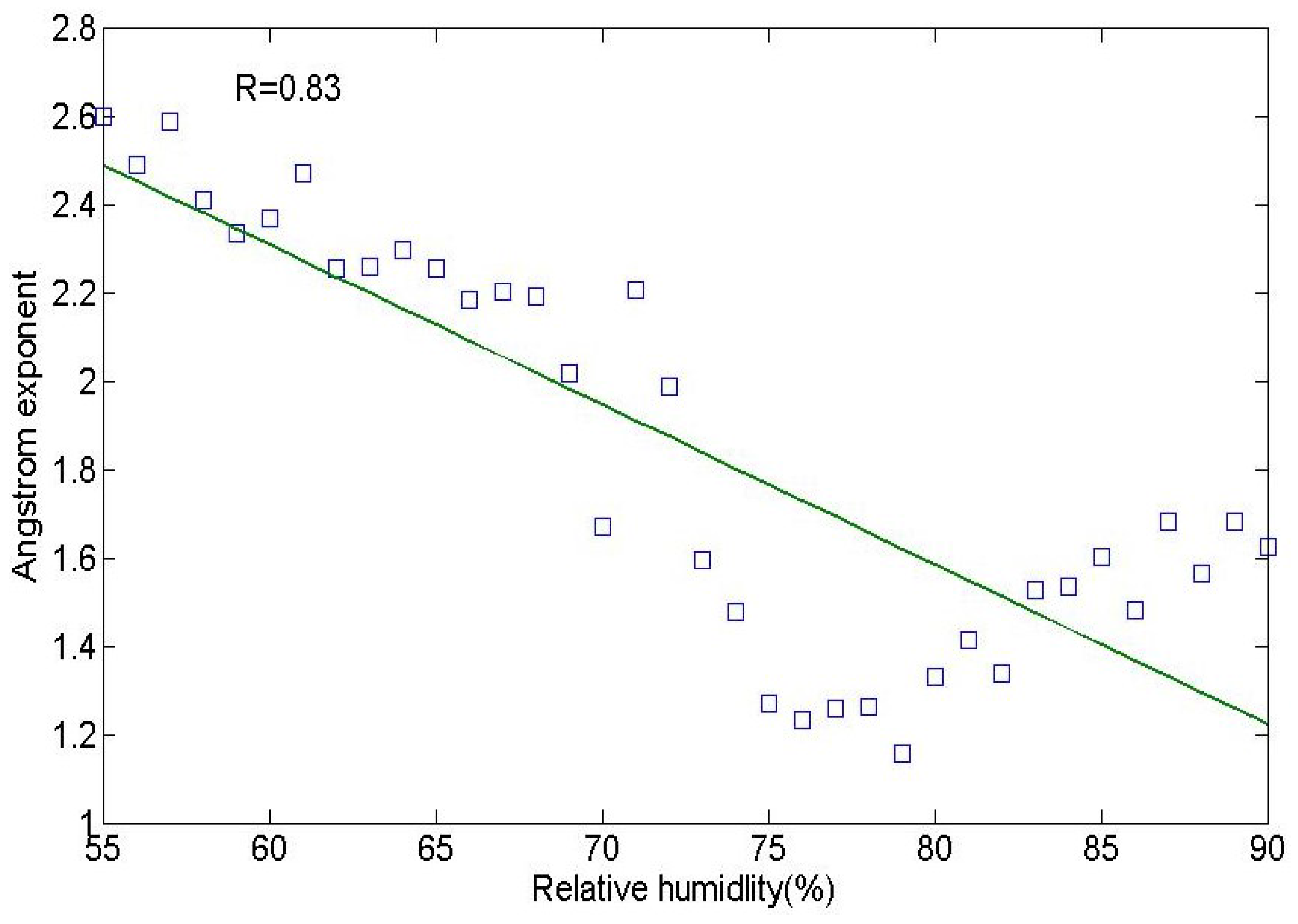
The variation of AE with the change of relative humidity during a portion of the time of the haze event is presented in
Figure 6. As
Figure 6 shows, AE decreased from 2.6 to 1.2 with the increase of relative humidity. The variation of AE corresponds with the hygroscopic growth of the aerosol, indicating that, as the aerosol size became larger due to hygroscopic growth, the AE simultaneously decreased. When the relative humidity reached 75%, the AE began to rise. The AE also showed a similar trend with extinction coefficient after the relative humidity of about 75%. These changes occurred because the larger particulates that resulted from hygroscopic growth were blown out by wind, and the newly generated particulates had smaller sizes. In conclusion, the AE and the relative humidity showed a negative correlation, with a correlation coefficient of 0.83 within the relative humidity range of 55% to 90%.
Figure 6.
Comparison between relative humidity and Angstrom exponent.
Figure 6.
Comparison between relative humidity and Angstrom exponent.
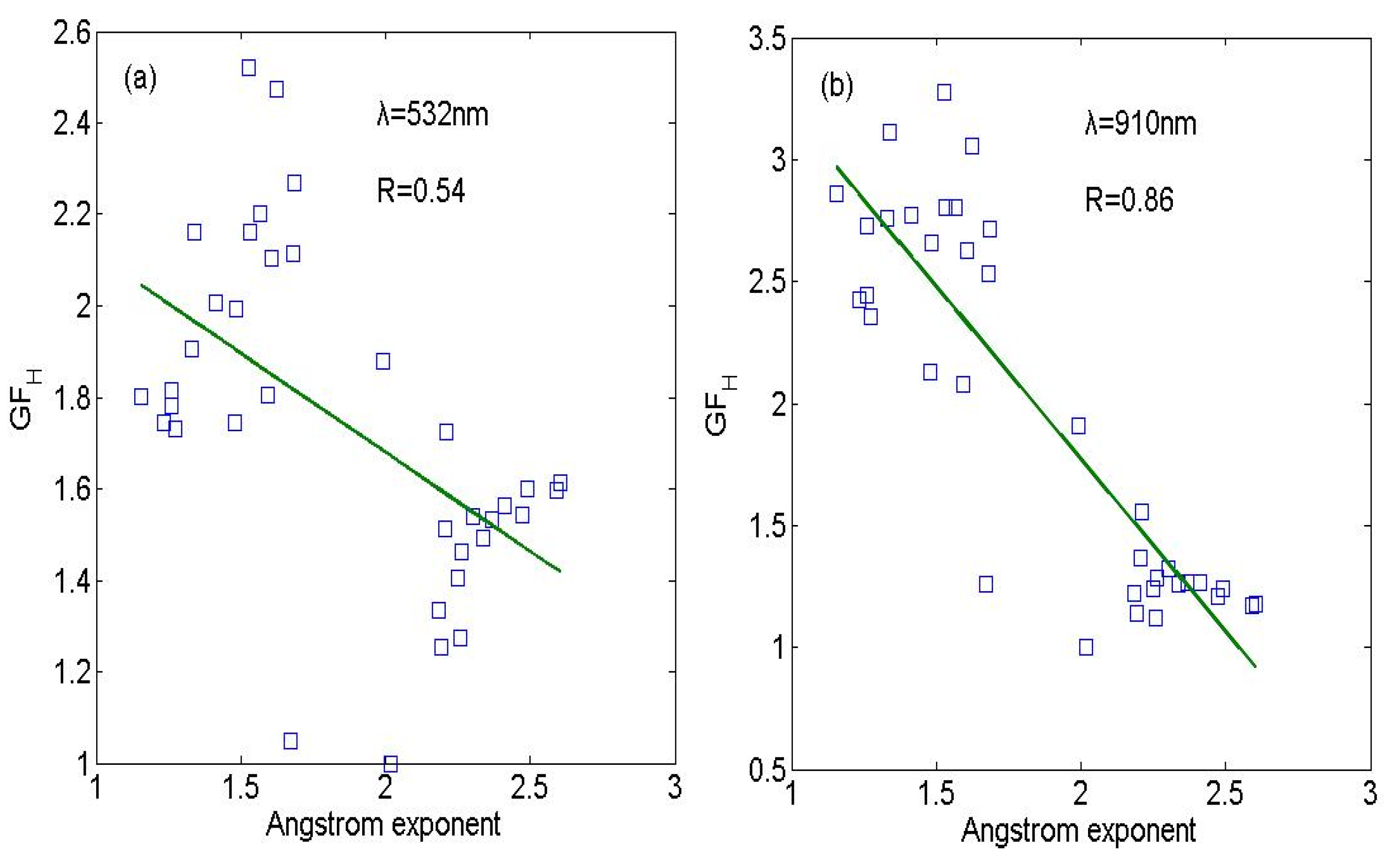
Figure 7 shows the relationship between the hygroscopic growth factor and the AE. During the time segment between 16:00 and 22:00 on 2 October 2014, in which the relative humidity increased gradually, the correlation coefficients at 532 nm and 910 nm were 0.54 and 0.86, respectively. The relationships show that the correlation between hygroscopic growth and that AE is higher at 910 nm than at 532 nm. The reason for the difference is that the 910 nm laser is more sensitive to the larger particulates. From the figure, it can be seen that, as relative humidity increased, the size of the particulates become larger and the AE become smaller.
Figure 7.
Comparison between hygroscopic growth factor and Angstrom exponent at (a) 532 nm and (b) 910 nm.
Figure 7.
Comparison between hygroscopic growth factor and Angstrom exponent at (a) 532 nm and (b) 910 nm.
3.5. Distribution Characteristics of Aerosol Particle Spectrum
Ulevicius
et al. reported the variations of the aerosol size distribution during the haze episode. Aerosol effects such as Brownian diffusion, collision, agglomeration, and deposition during the process of relative humidity change will result in spectrum distribution changes of atmospheric aerosol particles [
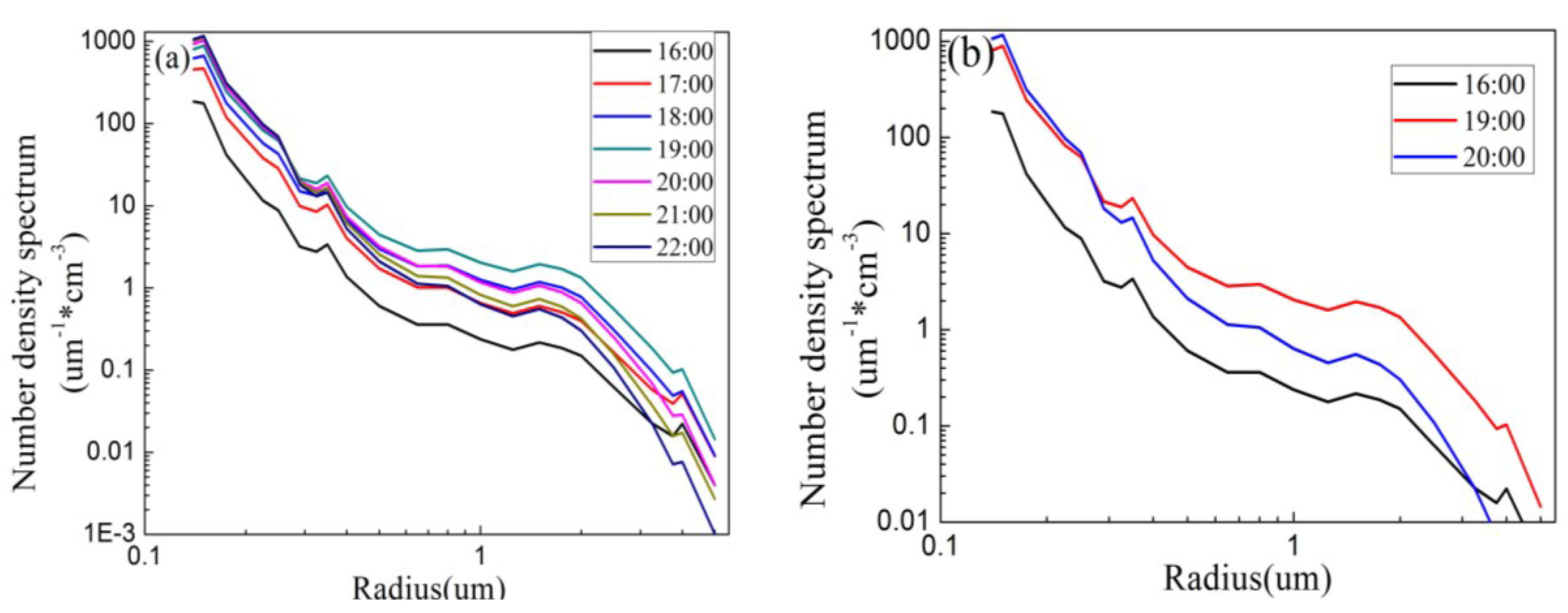
18]. A particle monitor (model: Grimm 180) was used to obtain aerosol particle concentrations at different aerosol sizes. The characteristics of the aerosol size distribution during the haze that occurred on 2 October 2014 were analyzed and are shown in
Figure 8. As shown in
Figure 8a, the peak for each time at the corresponding particle radius is basically the same. In the lower part of the accumulation mode (
r < 0.3 µm), the aerosol concentrations increase monotonously with time. However, the distribution of the larger particulates is more complex because this distribution has a relation with hygroscopic growth and other meteorological parameters, as mentioned previously. To demonstrate this phenomenon, the particulate distributions at three points in time are presented in
Figure 8b. From
Figure 8b, it can be seen that the distribution at 20:00 has the highest concentration of particles smaller than 0.3 µm, but the concentration of larger particulates is not the highest at 20:00. The particulate distributions show that the particulates with small size are stable, while the particulates with large size are unstable.
Figure 8.
Aerosol particle spectrum distribution during the fog-haze (a) and at three different points in time (b).
Figure 8.
Aerosol particle spectrum distribution during the fog-haze (a) and at three different points in time (b).
In
Figure 8b, the relative humidity is 55% at 16:00, 77% at 19:00, and 90% at 22:00. As shown in
Figure 8a, when the relative humidity is relatively lower at 16:00, the particle concentration is also relatively small, especially for fine particles within the size range of 0.15 µm to 0.8 µm. As the haze episode develops, the fine aerosol concentration increases rapidly to the blue curve in
Figure 8b. At 19:00 and 22:00, the fine mode radius (0.125–0.2 µm) particle concentrations are similar, but the coarse mode particle concentration is significantly greater at 19:00 than at 22:00. Mie theory was used to study the scattering characteristics of particles with different sizes. Firstly, we investigated the scattering characteristics of particles with a size of 1.5 µm. The Mie calculation results showed that the phase function at 532 nm has characteristic of large oscillation while scattering of 910 nm is more stable than that at 532 nm. In addition, a comparison between scattering characteristics of particles with a size of 1.5 µm and that of particles with a size of 2.5 µm was conducted. With particle size changes from 1.5 µm to 2.5 µm, the relative changes of scattering intensities at 532 nm and 910 nm were 66%, 89% respectively. Examining the change of AE with time on 2 October (
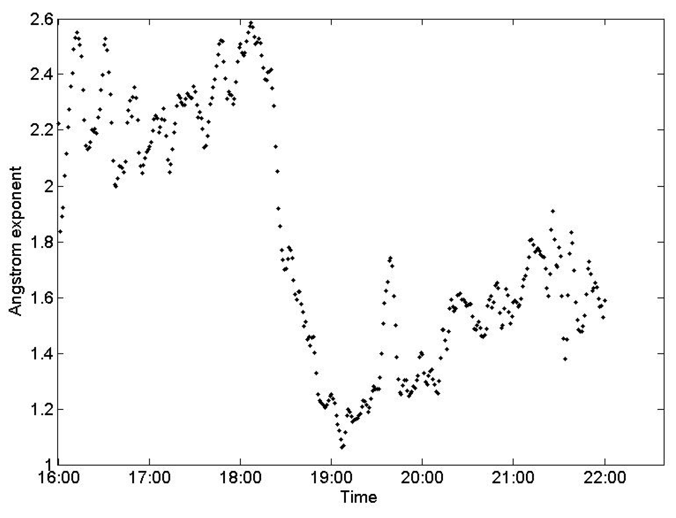
Figure 9), it can be seen that, because the coarse mode particle concentration begins to decrease at 19:00, the variation of AE changes to an upward trend. As mentioned previously, an analysis revealed that the decrease of the aerosol coarse mode particulate concentration occurred mainly because an increased wind blew away the particles that had grown larger. The effect of the wind caused the decrease of the coarse mode particles and the increase of the AE.
Figure 9.
Change of Angstrom exponent with time.
Figure 9.
Change of Angstrom exponent with time.
4. Conclusions and Discussion
Combining the data from the MPL (532 nm) and the CL31 (910 nm) ceilometers with the aerosol size distribution monitor, the characteristics of the aerosols during the haze episode were analyzed. For the two different wavelengths, the particles showed different optical characteristics, and the longer wavelength was more sensitive to larger particles. As well as it affects visibility, relative humidity showed a close relationship with hygroscopic growth and AE. The characteristics of the size concentration spectrum verified the analyzed results for hygroscopic growth and AE. From the results of this study, it can be concluded that more particulate characteristics than only optical characteristics can be retrieved from ceilometer data. Furthermore, the aforementioned ceilometer network will be constructed in the near future according to the schedule of the CMA. Based on the facts mentioned above, the haze in China, which is a serious social problem and often brings adverse effects, can be monitored more effectively by combining data from the ceilometer network with those from the existing particulate monitoring instruments.
Acknowledgments
The work was supported by the Natural Science Foundation of Jiangsu Province (Grant No. BK20141480 and Grant No. BE2015003-4) and the National Science Foundation of China (Grant No. 41304124).
Author Contributions
All authors contributed immensely. Jing Yuan collected and analyzed the data and wrote the paper. Lingbing Bu defined the major working scheme and modified the paper. Xingyou Huang provided key data. Haiyang Gao was in charge of the observation of optical parameters. Rina Sa processed and analyzed the haze data.
Conflicts of Interest
The authors declare no conflicts of interest.
References
- Zhang, Q.; Shen, Z.; Cao, J.; Zhang, R.; Zhang, L.; Huang, R.J.; Zheng, C.; Wang, L.; Liu, S.; Xu, H.; et al. Variations in PM2.5, TSP, BC, and trace gases (NO2, SO2, and O3) between haze and non-haze episodes in winter over Xi’an, China. Atmos. Environ. 2015, 112, 64–71. [Google Scholar] [CrossRef]
- Li, M.; Zhang, L. Haze in China: Current and future challenges. Environ. Pollut. 2014, 189, 85–86. [Google Scholar] [CrossRef] [PubMed]
- Zhang, M.; Ma, Y.Y.; Gong, W.; Zhu, Z. Aerosol optical properties of a haze episode in Wuhan based on ground-based and satellite observations. Atmosphere 2014, 5, 699–719. [Google Scholar] [CrossRef]
- Huang, X.; Yang, X.; Geng, F.; Zhang, H.; He, Q.; Bu, L. Aerosol measurement and property analysis based on data collected by a micro-pulse LIDAR over Shanghai, China. J. Opt. Soc. Korea 2010, 14, 185–189. [Google Scholar] [CrossRef]
- Pan, H.; Geng, F.H.; Chen, Y.H.; He, Q.; Zhang, H.; Kang, Y.; Mao, X.; Wang, H. Analysis of a haze event by micro-pulse light laser detection and ranging measurements in Shanghai. Acta Sci. Circumstantiae 2010, 30, 2164–2173. [Google Scholar]
- Zhang, W. Spatial and temporal variability of aerosol vertical distribution based on lidar observations: A haze case study over Jinhua basin. Adv. Meteorol. 2015, 2015, 349592. [Google Scholar] [CrossRef]
- Bu, L.B.; Yuan, J.; Gao, A.Z.; Lei, Y.; Guo, W.; Gao, H.; Huang, X. Analysis of haze-fog events based on laser ceilometer. Acta Photonica Sin. 2014, 43. [Google Scholar] [CrossRef]
- He, Q.S.; Mao, J.T. Micro-pulse lidar and its applications. Meteorological. Sci. Technol. 2004, 32, 219–224. [Google Scholar]
- Dai, Y.J.; Cai, X.P.; Chen, X.J.; Chen, Z.L. Micro pulse lidar for measuring clouds. Infrared Laser Eng. 2000, 29, 1–5. [Google Scholar]
- Grimm. Mobile Dust Monitor ENVIRON CHECK 180 User’s Guide; Grimm: München, Germany, 2010. [Google Scholar]
- Kleet, J.D. Stable analytical inversion solution for processing lidar returns. Appl. Opt. 1981, 20, 211–220. [Google Scholar] [CrossRef] [PubMed]
- Yin, K.X.; Fan, C.Y.; Wang, H.T.; Qiao, C.; Zhang, P. Aerosol extinction characteristics in haze and fine weather in southeast coastal area of China. High Power Laser Part. Beams 2015, 27. [Google Scholar] [CrossRef]
- Meier, J.; Wehner, B.; Massling, A.; Birmili, W.; Nowak, A.; Gnauk, T.; Brüggemann, E.; Herrmann, H.; Min, H.; Wiedensohler, A. Hygroscopic growth of urban aerosol particles in Beijing (China) during wintertime: A comparison of three experimental methods. Atmos. Chem. Phys. 2009, 9, 6865–6880. [Google Scholar] [CrossRef]
- Kotchenruther, R.A.; Hobbs, P.V.; Hegg, D.A. Humidification factors for atmospheric aerosols off the mid-Atlantic coast of the United States. J. Geophys. Res. Atmos. 1999, 104, 2239–2251. [Google Scholar] [CrossRef]
- Bo, G.Y.; Liu, D.; Wu, D.C.; Wang, B.; Zhong, Z.; Xie, C. Two-Wavelength Lidar for observation of aerosol optical and hygroscopic properties in fog and haze days. Chin. J. Lasers 2014, 41, 0113001. [Google Scholar]
- Liu, X.G.; Zhang, Y.H. Advances in research on aeroslo hygroscopic properties at home and abroad. Clim. Environ. Res. 2010, 15, 808–816. [Google Scholar]
- Chen, L.Y.; Jing, F.T.; Chen, C.H.; Hsiao, T. Hygroscopic behavior of atmospheric aerosol in Taipei. Atmos. Environ. 2003, 37, 2069–2075. [Google Scholar] [CrossRef]
- Ulevicius, V.; Trukmas, S.; Girgzdys, A. Aerosol size distribution transformation in fog. Atmos. Environ. 1994, 28, 795–800. [Google Scholar] [CrossRef]
© 2016 by the authors; licensee MDPI, Basel, Switzerland. This article is an open access article distributed under the terms and conditions of the Creative Commons by Attribution (CC-BY) license (http://creativecommons.org/licenses/by/4.0/).


