Solar Forecasting in a Challenging Insular Context

Abstract

This paper aims at assessing the accuracy of different solar forecasting methods in the case of an insular context. Two sites of La Réunion Island, Le Tampon and Saint-Pierre, are chosen to do the benchmarking exercise. Réunion Island is a tropical island with a complex orography where cloud processes are mainly governed by local dynamics. As a consequence, Réunion Island exhibits numerous micro-climates. The two aforementioned sites are quite representative of the challenging character of solar forecasting in the case of a tropical island with complex orography. Hence, although distant from only 10 km, these two sites exhibit very different sky conditions. This work focuses on day-ahead and intra-day solar forecasting. Day-ahead solar forecasts are provided by the European Center for Medium-Range Weather Forecast (ECMWF). This organization maintains and runs the Numerical Weather Prediction (NWP) model named Integrated Forecast System (IFS). In this work, post-processing techniques are applied to refine the output of the IFS model for day-ahead forecasting. Statistical models like a recursive linear model or a nonlinear model such as an artificial neural network are used to produce the intra-day solar forecasts. It is shown that a combination of the IFS model and the neural network model further improves the accuracy of the forecasts.

1. Introduction

Accurate solar forecasts at various time steps are needed in order to increase the integration of renewables into electricity grids [1]. This statement is reinforced in the case of insular grids. The fluctuating character of the solar energy together with the fact that the island electricity grid is isolated may put in danger the stability of the grid and consequently the balance between supply and demand.

In addition, solar forecasting may be very challenging in an insular context as islands (like Réunion Island for instance) may usually experience a high spatial and temporal variability of the solar resource [2]. Previous works regarding irradiance forecasting for the power PV prediction of grid-connected systems were mainly done for large-scale continental grids [3,4,5]. Due to the small scale of the climatic phenomena, forecasting the solar irradiance in insular territories addresses new issues.

In order to cope with specific plant operations, solar forecasts must be provided with different granularities and horizons [6]. In addition, the recent development of grid-connected storages associated with intermittent renewables (solar, wind and wave) also requires power PV forecasts in order to optimize their operational management [7,8]. PV power output is directly related to the level of received global solar irradiance. Thus, forecasting the global solar irradiance is the key feature for power PV forecasting. In this work, we will focus on day-ahead and intra-day solar irradiance forecasts with an hourly granularity.

For day ahead forecasting, the most accurate forecasting methods are based on Numerical Weather Prediction (NWP) models [1,9]. For forecast horizons up to several hours, models based on cloud-motion vectors (CMVs) from satellite images are the most suitable [10,11]. In addition, finally, for very short-term horizons, from few minutes up to six hours, the literature is dominated by statistical approaches based on linear or nonlinear models [12,13,14,15,16].

NWP models may exhibit (large) biases [9]. Post-processing methods like Model Output Statistics (MOS) are frequently applied to reduce these biases or to refine the output of NWP models, as detailed local weather features are generally not resolved by NWP predictions [3]. In addition, spatial averaging can contribute to reduce forecast errors, particularly in situations with variable clouds, that are difficult to predict ([4,17]). To our best knowledge, these post-processing techniques have been only tested in a continental context ([3,4,5]) and it appears interesting to assess in this survey the performances of these techniques in the case of an insular environment. In this work, day-ahead forecasts are provided by the European Center for Medium-Range Weather Forecast (ECMWF). This organization maintains and runs the global Numerical Weather Prediction (NWP) model Integrated Forecast System (IFS). Two post-processing techniques will be used to refine the IFS forecasts for the insular sites of Saint-Pierre and Le Tampon in Réunion Island.

Regarding the intra-day solar forecasting, two statistical models namely an Artificial Neural Network (ANN) and a recursive linear technique (ARMA.RLS) will be evaluated. Furthermore, some day-ahead parameters produced by ECMWF will be used as exogenous inputs of the ANN model. It will be shown that the combination of the IFS model and the ANN model further improves the accuracy of the forecasts.

The remainder of this paper is organized as follows: Section 2 is devoted to the sites’ description and data preprocessing. Section 3 sets out an in-depth analysis of the sky conditions experienced by each site while Section 4 will detail the errors metrics used to assess the forecasting accuracy of the different methods. Section 5 describes the day-ahead solar forecasts with a special emphasis on the MOS post-processing techniques. Section 6 presents the results of the intra-day solar forecasting techniques. Finally, Section 7 gives some concluding remarks.

2. Sites Description and Data Preprocessing

2.1. Sites Description

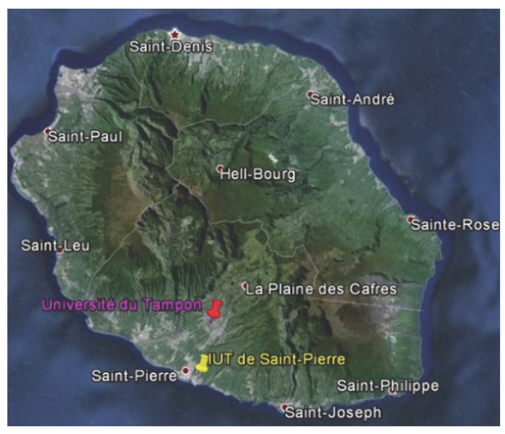
Réunion Island exhibits a particular meteorological context dominated by a large diversity of micro-climates. Two main regimes of cloudiness are superposed: the clouds driven by synoptic conditions over the Indian Ocean and the orographic cloud layer generated by the local reliefs [2]. The data used to build the models are Global Horizontal Irradiance (GHI) measured by the PIMENT laboratory at the meteorological stations of Saint-Pierre and Le Tampon located in the southern part of Réunion Island (see Figure 1). Saint-Pierre is a coastal site while Le Tampon is an inland site. Table 1 gives the sites’ characteristics.

Figure 1. The distance between the two sites: Saint-Pierre and Le Tampon is only about 10 km.

Figure 1. The distance between the two sites: Saint-Pierre and Le Tampon is only about 10 km.

Table 1. Sites characteristics, input parameters for the BIRD model and performance of the BIRD model. rRMSE and rMBE are normalized to mean measured irradiance (705 W/m² for Saint-Pierre and 649 W/m² for Le Tampon).

Site	Saint-Pierre	Le Tampon
Period of record	01/01/2012–31/12/2013	01/01/2012–31/12/2013
Longitude	55.491°E	55.506°E
Latitude	21.340°S	21.269°S
Elevation (m)	75	550
Annual solar irradiance (MWh/m2)	2.053	1.712
Average Pressure (Pa)	100,427	94,890
Ozone (cm)	0.2655	0.2655
Water vapor (cm)	2.933	2.933
AOD 500 nm (cm)	0.072	0.072
AOD 380 nm (cm)	0.090	0.090
Asymmetry factor Ba (see [20] for details)	0.84	0.84
Site variability (see Equation (2))	0.19	0.24
Nb. of clear sky hours	2614	1022
Bird clear sky model accuracy by Ineichen method [24] rRMSE	3.26%	4.52%
Bird clear sky model accuracy by Ineichen method [23] rMBE	1.7%	−1.9%

Table 1. Sites characteristics, input parameters for the BIRD model and performance of the BIRD model. rRMSE and rMBE are normalized to mean measured irradiance (705 W/m² for Saint-Pierre and 649 W/m² for Le Tampon).

Site	Saint-Pierre	Le Tampon
Period of record	01/01/2012–31/12/2013	01/01/2012–31/12/2013
Longitude	55.491°E	55.506°E
Latitude	21.340°S	21.269°S
Elevation (m)	75	550
Annual solar irradiance (MWh/m2)	2.053	1.712
Average Pressure (Pa)	100,427	94,890
Ozone (cm)	0.2655	0.2655
Water vapor (cm)	2.933	2.933
AOD 500 nm (cm)	0.072	0.072
AOD 380 nm (cm)	0.090	0.090
Asymmetry factor Ba (see [20] for details)	0.84	0.84
Site variability (see Equation (2))	0.19	0.24
Nb. of clear sky hours	2614	1022
Bird clear sky model accuracy by Ineichen method [24] rRMSE	3.26%	4.52%
Bird clear sky model accuracy by Ineichen method [23] rMBE	1.7%	−1.9%

2.2. Solar Radiation Data

Measurements are available on an hourly basis and two years of data (2012 and 2013) are used respectively for the building and appraisal of the models. The stations measure the GHI every six seconds and the 1-min averages are recorded. The hourly data correspond to the average of the previous 60 min of measurements. The solar irradiance is measured with a secondary standard pyranometer (CMP 11 from Kipp and Zonen). The uncertainty of the pyranometers is ±3.0% for the daily sum of GHI. Measurement quality is an essential asset in any solar resource forecasting study. The sites of Saint-Pierre and Le Tampon are well maintained and have followed the radiometric techniques regarding calibration, maintenance and quality control. Each data point has been processed with SERI-QC quality control procedure [18].

In this work, for comparison purposes, we also include two continental US sites namely Desert Rock (36.6N; 116.0W; 1007 m·a.s.l) and Fort Peck (48.3N; 105.1W; 634 m·a.s.l). These two stations are part of the NOAA’s SURFRAD network [19].

2.3. Clear Sky Index

Solar irradiance is characterized by diurnal and seasonal variations. A clear sky model is commonly used to remove this deterministic component in the GHI time series then leading to the definition and use of the clear sky index $k{t}^{*}$:

$$k{t}^{*}=\frac{GHI}{GH{I}_{Clear}}$$

(1)

It corresponds to the ratio of the measured GHI to the theoretical GHI observed under clear sky conditions $(GH{I}_{Clear})$. With this methodology, the models designed in this work are dedicated to the forecasting of the stochastic part of the global radiation due to the cloud cover, leaving the geometric and the deterministic part to be modeled by the clear sky model.

The clear sky irradiance is generated with the BIRD model [20]. This simple model calculates estimates of $GH{I}_{Clear}$with acceptable accuracy and with only few inputs [21]. For this study, the Aerosol Optical Depths (AODs) and the water vapor column parameters were retrieved from the AERONET site REUNION_ST_DENIS (20°52’S; 55°28’) [22] located in the north of the island. 4.5 years were used to compute the climatological means of these atmospheric input parameters. The latter were used as inputs of the BIRD model. Similarly, the ozone atmospheric content was retrieved from the World Ozone Monitoring Mapping provided by the Canadian government [23]. The values of the input parameters of the BIRD model used for the two studied sites are given in Table 1.

The forecasting accuracy of the models proposed in this work depends on the accuracy of the clear sky model used to derive the clear sky index. In order to evaluate this error induced by the BIRD model, only the clear sky periods are considered. The clear sky hours were detected using the Ineichen method [24] applied to the two years of hourly-measured global irradiance. The last three lines of Table 1 give the number of clear sky hours detected, the relative Root Mean Square Error (rRMSE) and the relative Mean Bias Error (rMBE)—see the definition of these metrics below of the corresponding clear sky irradiance produced by the BIRD model. The performances of the BIRD model in this work are consistent with previous results [25]. Notice also that the site of Le Tampon experiences fewer occurrences of clear sky hours (see Table 1).

2.4. Filtering Methodology

Low solar elevations induce complex reflection phenomena that are not properly taken into account by the pyranometer. As a consequence, the values of the measured GHI are often not reliable. Furthermore, the amount of solar energy received at ground level in this condition is very small. As a consequence, data corresponding to a solar zenith angle (${\mathsf{\Theta }}_Z$) larger than to 85° are removed. This filtering removes less than 1% of the total annual sum of solar energy. Put in other words, night times and low solar elevations were not taken into account for the building and the test of the models. In addition, this filtering process allows to discard data with less precision as measurement uncertainties associated to pyranometers are typically much higher than ±3.0% for ${\mathsf{\Theta }}_Z$ > 85°.

3. Sites Analysis

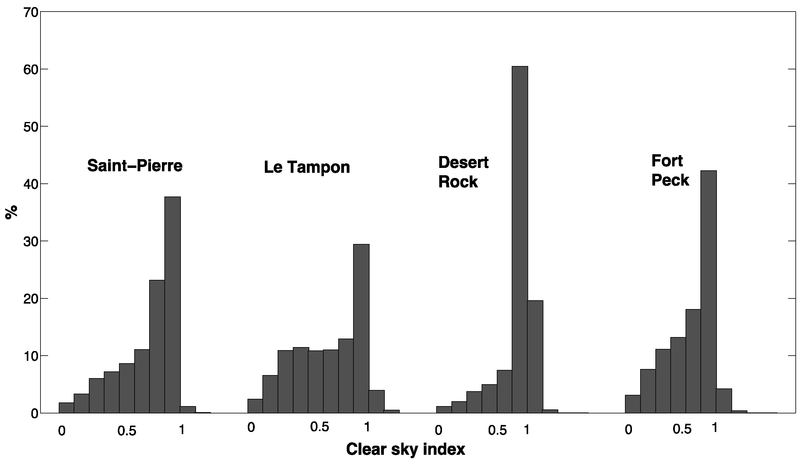
This section aims at analyzing the sky conditions experienced by each site. Figure 2 plots the distribution of the clear sky index for each site. In Table 2, based on the previous work done by [26], we define thresholds to distinguish different sky conditions.

Table 2. $k{t}^{*}$ Values and related sky conditions.

kt* Values	Sky Conditions
$k{t}^{*}>0.8$	Clear
$0.35<k{t}^{*}<0.8$	Cloudy/intermediate
$k{t}^{*}<0.35$	Overcast

Table 2. $k{t}^{*}$ Values and related sky conditions.

kt* Values	Sky Conditions
$k{t}^{*}>0.8$	Clear
$0.35<k{t}^{*}<0.8$	Cloudy/intermediate
$k{t}^{*}<0.35$	Overcast

We also include in Figure 2, the $k{t}^{*}$ distribution of the two continental sites namely Desert Rock and Fort Peck. The site of Desert Rock is representative of an arid climate dominated by clear skies. One may also notice that the $k{t}^{*}$ distributions of the sites of Fort Peck and Saint-Pierre are quite similar. Indeed, as mentioned above, Saint-Pierre is a coastal site with rather high occurrences of clear skies. Conversely, the site of Le Tampon exhibits higher occurrences of cloudy/intermediate skies.

The characterization of the variability regime of solar irradiation at a particular site is a key factor to understand the level of error of a solar forecasting method. Put in other words, the variability experienced by a site has an impact on the forecasting accuracy of the different forecasting methods.

Table 1 gives a metric that characterizes the annual solar variability of a site. This metric proposed by [27] is the standard deviation of the change in the clear sky index defined by:

$$\sigma \left(\Delta k{t}_{ \Delta t}^{*}\right)=\sqrt{Var\left[\Delta k{t}_{ \Delta t}^{*}\right]}$$

(2)

Figure 2. Statistical distribution of the 1-hour clear sky index for the 2 considered insular locations and the two continental sites.

Figure 2. Statistical distribution of the 1-hour clear sky index for the 2 considered insular locations and the two continental sites.

The values of solar variability in Table 1 have been calculated for a time scale $\Delta \mathrm{t}=1$ h (as we deal with hourly GHI records) and for a time span that corresponds to two years of hourly data. A site with variability above 0.2 is considered as experiencing very unstable conditions [27,28].

As seen, the variability of the site of Le Tampon is above this threshold. Conversely, the variability of Desert Rock and Fort Peck are respectively 0.14 and 0.18. One may also notice that the variability of Saint-Pierre is close to that of Fort-Peck. Sub-Section 6.5.2 below will discuss the impact of the sky conditions on the forecasting accuracy of the different methods.

4. Error Metrics

In the realm of the solar forecasting community, the commonly used error metrics for point forecasts are: the Root Mean Square Error (RMSE), Mean Absolute Error (MAE) and Mean Bias Error (MBE). These error metrics are defined by the following equations:

$$RMSE=\sqrt{\frac{1}{N}{\displaystyle \sum }_{i=1}^N{\left(GH{I}_{forecast.i}-GH{I}_{measured.i}\right)}^2}$$

(3)

$$MAE=\frac{1}{N}{\displaystyle \sum }_{i=1}^N\left|GH{I}_{forecast.i}-GH{I}_{measured.i}\right|$$

(4)

$$MBE=\frac{1}{N}{\displaystyle \sum }_{i=1}^N\left(GH{I}_{forecast.i}-GH{I}_{measured.i}\right)$$

(5)

where N is the number of points in the dataset for the considered period.

Relative values of these metrics (rRMSE, rMAE and rMBE) are obtained by normalization to the mean ground measured irradiance of the considered period. As noted by Lorenz in [1], the MAE is appropriate for applications with linear cost functions, that is, where the costs that are caused by a wrong forecast are proportional to the forecast error. The RMSE is more sensitive to large forecast errors, and hence is suitable for applications where small errors are more tolerable and larger errors cause disproportionately high costs. In the following, we provide the standard set of error metrics but with a special emphasis on the rRMSE.

In this work, we also include an additional metric: the forecast skill parameter s. The latter proposed by [29] is given by $s\left(\%\right)=\left(1-\frac{RMS{E}_{method}}{RMS{E}_{pers}}\right)\times 100$ where $RMS{E}_{method}$stands for the RMSE of each new proposed forecasting method and $RMS{E}_{pers}$ is the RMSE of the persistence model. With this definition, the persistence model has a forecast skill s = 0% and a value of s = 100% denotes a perfect forecast. Negative values of s indicate that the forecasting model fails to outperform the persistence model while positive values of s means that the forecasting method improves on persistence. Further, the higher the s-skill score is, the better the improvement is.

5. Day-Ahead Forecasting

5.1. Initial ECMWF Forecast

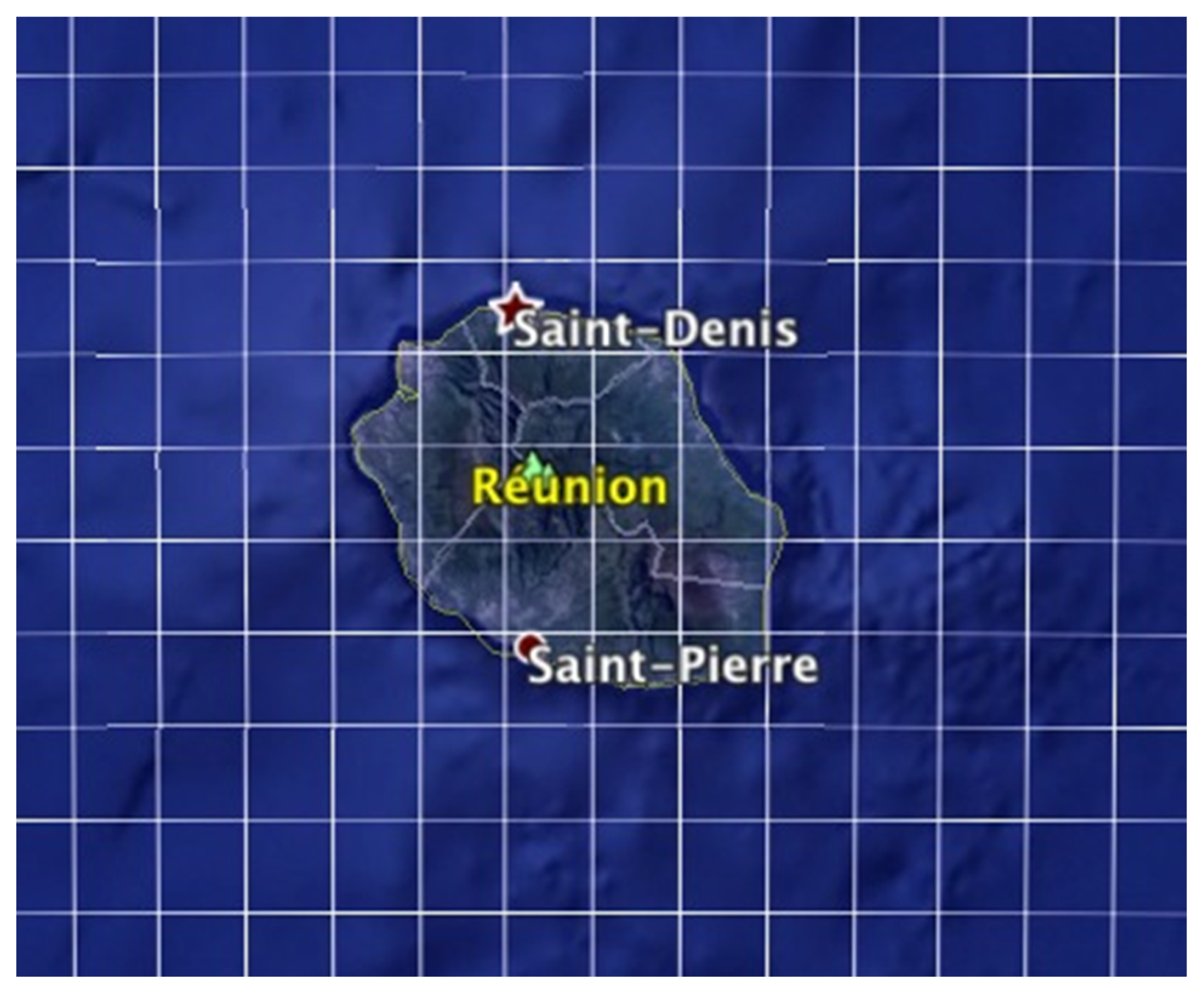
The European Center for Medium-Range Weather Forecast (ECMWF) is an intergovernmental organization that provides operational forecasts. It maintains and runs the numerical weather prediction (NWP) model Integrated Forecast System (IFS). NWP models outperform forecasts based on satellite data or ground measurements (only) for horizons longer than 5 h [1,11]. In order to supply forecasts that can be used by the grid operator for day-ahead scheduling, we retrieved the data generated by the IFS at 12 h 00 UTC (16 h 00 in Réunion Island). The forecasts correspond to hourly data with a spatial resolution of 0.125° × 0.125° (approximately 14 km × 14 km in Réunion—see Figure 3).

Figure 3. ECMWF grid for La Réunion Island.

Figure 3. ECMWF grid for La Réunion Island.

5.2. Post-Processing the IFS Model

In order to obtain an optimized local prediction, post-processing techniques are used to refine the output of NWP models. More precisely, post-processing the NWP model output consists in using a statistical method (also called Model Output Statics (MOS)) to correct systematic deviations due to either model errors or local influences not resolved by the NWP model. Indeed, although spatial resolution has increased during the last years, the NWP models still do not resolve the local weather details [1]. Therefore, there is room for improvement as regards the original NWP forecasts.

For the case study of Germany, Lorenz et al. [3] showed that the ECMWF forecasts could be refined with a MOS technique that consisted of a bias correction. In this work, a prior step to this bias correction was to apply a spatial averaging procedure on the original ECWMF forecasts.

5.2.1. Spatial Averaging

Spatial averaging of irradiance forecasts can lead to improved forecasts (notably in terms of RMSE) by smoothing the variations in variable sky conditions (due to changing cloud cover) [3,17]. For the site of Saint-Pierre and Le Tampon, we applied the spatial averaging technique (i.e., arithmetic average of surrounding pixels) to potentially improve the accuracy of the day-ahead forecasts. As shown by Figure 4, the spatial averaging technique did not improve the forecast accuracy. Unlike [3] which obtained the lowest RMSE by averaging over 4 × 4 pixels, here, the lowest RMSE is obtained for the nearest pixel. This result may come from the small scale of the island or also because the average predictions for land and surrounding ocean are mixed. Therefore, we can conjecture that the spatial averaging of the global IFS forecasts may be irrelevant in the case of small insular territories.

Figure 4. Spatial averaging of the day-ahead ECMWF forecasts around Saint-Pierre.

Figure 4. Spatial averaging of the day-ahead ECMWF forecasts around Saint-Pierre.

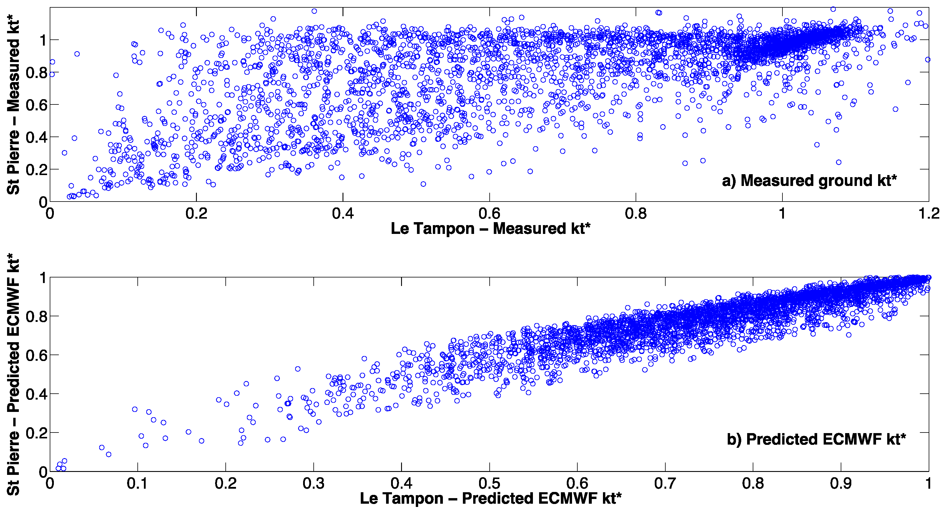
In order to further illustrate the challenging character of solar forecasting in the case of a small tropical island with complex orography, Figure 5a plots the ground observations of Saint-Pierre vs. the ground observations of Le Tampon. As seen, although there is a small distance between the two sites, the discrepancy between the two ground measurements is relatively important. A correlation coefficient of 0.64 calculated between the two $k{t}^{*}$ time series of each site reinforces this statement. As shown by Figure 5b, it is not the case for the ECMWF forecasts. A correlation coefficient of 0.96 confirms that the ECMWF forecasts are rather similar for the two sites as a consequence of the coarse spatial resolution of ECMWF for a territory like Réunion Island.

Figure 5. (a) Comparison of the measured $k{t}^{*}$for the two sites; (b) Comparison of the predicted ECMWF $k{t}^{*}$ for the two sites.

Figure 5. (a) Comparison of the measured $k{t}^{*}$for the two sites; (b) Comparison of the predicted ECMWF $k{t}^{*}$ for the two sites.

5.2.2. Bias Correction with An Artificial Neural Network

Consistent error patterns allow for MOS to be used to produce a bias reduction function for future forecasts. In the case of Germany, as the original ECMWF forecasts showed a considerable overestimation of irradiance for intermediate sky conditions, Lorenz et al. [3] modeled the bias correction function by a polynomial function of fourth order in the variables $\widehat{{\mathrm{k}}_{\mathrm{t}}^{*}}$(predicted ECMWF clear sky index) and the cosine of the solar zenith angle ($\cos {\mathsf{\Theta }}_{\mathrm{Z}}$). The corrected forecast is then obtained by subtracting the modeled bias from the original predicted values. This approach eliminated bias and reduced root mean square error (RMSE) of hourly forecasts by 5% for 24 h forecasts. Similarly to [3], we implement a bias correction, but based on an Artificial Neural Network (ANN) model instead of a polynomial model, which allows considering additional input variables

ANNs are data driven approaches capable of performing a non-linear mapping between sets of input and output variables. An ANN with d inputs, m hidden neurons and a single linear output unit defines a non-linear parameterized mapping from an input vector $x=\left(x_1,x_2,\cdots ,x_d\right)$ to an output y given by the following relationship:

$$y\left(x;w\right)={\displaystyle \sum }_{j=1}^m{w}_{j}f\left({\displaystyle \sum }_{i=1}^d{w}_{ji}{x}_i+b_1\right)+b_2$$

(6)

Each of the m hidden units are related to the tangent hyperbolic function $f\left(x\right)=\left(e^x-e^{-x}\right)/\left(e^x+e^{-x}\right)$. The parameter vector $w=\left(\left\{w_j\right\},\left\{w_{ji}\right\},b_1,b_2\right)$ governs the non-linear mapping and is estimated during a phase called the training or learning phase. During this phase, the ANN is trained by the scaled conjugate gradient algorithm using a dataset (called training set) of N input and output examples. The second phase, called the generalization phase, consists of evaluating the ability of the ANN to generalize, that is to say, to give correct outputs when it is confronted with examples that were not seen during the training phase. Careful attention must be put on the building of the model, as a too complex ANN will easily overfit the training data. Several techniques like pruning [30], Bayesian regularization [31] or multi-objective genetic algorithm [32] can be employed to control the ANN complexity. In this work, we used the Bayesian Technique in order to automatically control the ANN complexity and therefore improve the generalization capability of the model [31]. The Bayesian approach offers significant advantages over the classical ANN learning process. Among others, one can cite the optimization of the ANN model using only the training dataset (i.e., no independent or validation dataset is needed). In addition, the Bayesian method offers a means to select the optimal number of hidden nodes by performing a model comparison. The interested reader is referred to [31] for details regarding the Bayesian approach.

In our application, we used a feed-forward ANN with only one hidden layer as it was theoretically proven that only one layer is sufficient to approximate any continuous function [33]. The ANN output y (i.e., the modeled bias) is related to three input variables namely the predicted clear sky index ($\widehat{{\mathrm{k}}_{\mathrm{t}}^{*}}$), the cosine of the zenith angle ($\cos {\mathsf{\Theta }}_{\mathrm{Z}}$) and the predicted total cloud cover ($\widehat{\text{TCC}}$). The MOS-corrected ECWMF forecasts are then obtained by subtracting the modeled bias from the original ECMWF forecasts.

5.3. Results of Day-Ahead Solar Forecasting and Discussion

An operational experimental set-up was used to implement the bias correction over the year 2012. More precisely, a sliding window of 90 days was used to train the ANN model and the bias correction was tested on the next day following the sliding window. In addition, let us recall that this MOS correction is not applied for ${\mathsf{\Theta }}_{\mathrm{Z}}$ > 85°. We compare our approach with the MOS technique employed by [3]. Let us recall that, in this previous work, the bias correction function was a polynomial of fourth order in the variables clear sky index ($\widehat{{\mathrm{k}}_{\mathrm{t}}^{*}}$) and the cosine of the zenith angle ($\cos {\mathsf{\Theta }}_{\mathrm{Z}}$). Table 3 lists the values of the error metrics.

As shown by Table 3, post-processing of the day-ahead forecasts produced by ECMWF allows improving their quality. Indeed, the bias of the corrected ECMWF forecasts is efficiently reduced. However, a relatively small improvement is observed for the quadratic error (rRMSE), which is in agreement with [3]. Overall, the ANN technique performs slightly better than the polynomial model. This improvement may come from the adding of the Total Cloud Cover (TCC) as a third input variable. Further, the MOS technique based on the 4th order polynomial model is a linear parameterized model while the ANN model is able to reproduce more complex non-linear relationships between the inputs and the output.

Table 3. Relative errors of the day-ahead forecasts.

Location	Saint-Pierre			Le Tampon
Year	2012			2013
Mean GHI (W·m−2)	490			429
Relative error (%)	rMBE	rRMSE	rMAE	rMBE	rRMSE	rMAE
Original ECMWF forecasts	−5.3%	29.2%	21.2%	5.6%	41.9%	29.8%
ECMWF + Polynomial bias correction	−1.1%	28.9%	20.6%	−0.6%	39.9%	29.9%
ECMWF + ANN bias correction	−1.0%	28.1%	19.6%	−1.0%	39.0%	28.8%

Table 3. Relative errors of the day-ahead forecasts.

Location	Saint-Pierre			Le Tampon
Year	2012			2013
Mean GHI (W·m−2)	490			429
Relative error (%)	rMBE	rRMSE	rMAE	rMBE	rRMSE	rMAE
Original ECMWF forecasts	−5.3%	29.2%	21.2%	5.6%	41.9%	29.8%
ECMWF + Polynomial bias correction	−1.1%	28.9%	20.6%	−0.6%	39.9%	29.9%
ECMWF + ANN bias correction	−1.0%	28.1%	19.6%	−1.0%	39.0%	28.8%

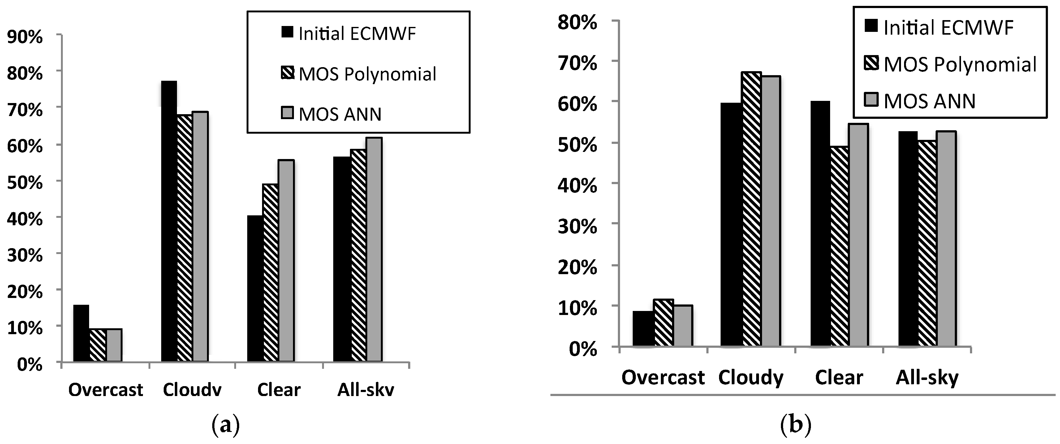
In addition, we analyze the capability of the different models to distinguish between different sky conditions: clear sky, cloudy sky and overcast sky, defined by the thresholds given in Table 2. A forecast correctly predicting the sky conditions, i.e., falling in the same range of the measured clear sky index according to Table 2 is labeled as “good” forecast in the following. In other words, a “good” forecast corresponds to a correctly predicted event or state.

Figure 6 shows the percentage of “good” forecasts for the initial ECMWF model and for the two post-processing methods. In this figure, the percent value is the number of correctly predicted states over the number of states as measured. As shown by Figure 6, according to the site under study, the behavior of the post-processing techniques is different. For the site of Saint-Pierre, the MOS techniques increase the rate of “good” forecasts in case of clear sky. However, the MOS techniques also reduced the percentage of “good” forecasts in case of cloudy or overcast skies. For Le Tampon, the bias correction method increases the rate of “good” forecasts in case of cloudy or overcast skies but decreases this rate in case of clear skies. Figure 6 gives also the number of correct forecasts for all-sky conditions. For Saint-Pierre, the overall share of correctly predicted events by the post-techniques is increasing. However, for le Tampon, no improvement is observed. Overall, regarding the two post-processing techniques, it appears again that ANN performs slightly better than the polynomial model.

Finally, while the MOS correction method led to a significant bias reduction, it appears that more work must be done in order to improve the results. As a bias correction can only correct systematic deviations, some original “good” forecasts have been unnecessarily corrected. Future work may consist in carrying an in-depth study of the error analysis that could pinpoint in detail the origin of the errors. This detailed bias analysis may lead (in addition to the clear sky index, TCC and $\cos {\mathsf{\Theta }}_{\mathrm{Z}}$) to the identification of another relevant input variables for the ANN.

Figure 6. Rate of “good” forecasts before and after the post-processing for three different sky conditions. (a) Saint-Pierre; (b) Le Tampon.

Figure 6. Rate of “good” forecasts before and after the post-processing for three different sky conditions. (a) Saint-Pierre; (b) Le Tampon.

6. Intra-Day Forecasting

6.1. Reference Models

Following Perez et al. [11], we propose to test our forecasting methods against reference models like persistence, smart persistence and climatology.

The persistence (Pers) model is expressed as follows:

$$\widehat{k{t}^{*}}\left(t+h\right)=k{t}^{*}\left(t\right)$$

(7)

Notice that in all the following equations describing the forecasting models, we used the following notations: a variable with a hat (^) is a forecasted variable, h = 1,2,3,…6 is the forecasting time horizon also called the lead time and t denotes the time when the forecasts are generated.

This model assumes that the clear sky index for each time horizon h depends only on the previous measured value $k{t}^{*}\left(t\right)$, which means that the sky conditions remain invariant between time ‘t’ and time ‘t + h’. The next model represents an easy way to improve the persistence model and it is called Smart Persistence (Smart-Pers). It consists in forecasting the clear sky index for each time horizon ‘h’ as the mean of the ‘h’ previous measured clear sky values. Smart-persistence model is defined by the following equation:

$$\widehat{k{t}^{*}}\left(t+h\right)=mean\left[k{t^{*}}_{\left(t\right)}.\dots .k{t^{*}}_{\left(t-h\right)}\right]$$

(8)

Finally, we propose the climatological mean model, which is independent of the forecasting time horizon. More precisely, this model performs a constant forecast of the clear sky index that corresponds to its mean historical value:

$$\widehat{k{t}^{*}}\left(t+h\right)=mean \left(k{t}^{*}\right)$$

(9)

Unlike persistence, it presents a limit in terms of accuracy for longer horizons. In our case, we used the average clear sky index of the year 2012 in order to forecast the clear sky index of the year 2013.

6.2. Intra-Day Solar Forecasts with A Linear Recursive Model (ARMA.RLS Model)

The Auto Regressive Moving Average (ARMA) model is a popular linear technique in the realm of solar forecasting. In particular, it has been extensively studied in renewable energy forecasting and, owing to its parsimony, it has turned out to be a very tough competitor to beat. Applications include, among others, forecasting of wind power generation [34], online power forecasting [35] and wave energy flux [36].

A general formulation of an ARMA (p,q) model with p autoregressive (AR) terms and q moving average (MA) terms is given by [37]:

$$\widehat{k{t}^{*}}\left(t+h\right)={\theta }_0+{\displaystyle \sum }_{i=1}^p{\theta }_{i}k{t}^{*}\left(t-i+1\right)+\epsilon \left(t\right)+{\displaystyle \sum }_{j=1}^q{\varphi }_j\epsilon \left(t—j\right)$$

(10)

$ϵ\left(t\right)$ is an independent and identically distributed random variable with a zero mean. The vector $\mathsf{\Theta }=\left({\mathsf{\theta }}_0.{\mathsf{\theta }}_1.\cdots .{\mathsf{\theta }}_{\mathrm{p}}.{\mathsf{\Phi }}_{1.}.\cdots .{\mathsf{\Phi }}_{\mathrm{q}}\right)$ contains the set of parameters to be estimated. A classic setting based on a least-squares method and a training data set can be used to estimate the set of parameters [37].

However, in this work, to estimate the model’s parameters, we chose a variation of the least squares method, namely the Recursive Least Square (RLS) method (see [38] for details of implementation). This method offers the advantage of reducing the computational cost for estimating the model’s parameters. In addition, the parameters are updated in real-time as new data become available. This contrasts with more intensive estimation methods operating on a sliding window where the estimation process is being carried out at each time step. Hence, the RLS method is particularly well suited in an operational context where forecasts have to be timely delivered. In addition, it must be stressed that contrary to non-linear models like ANNs, no training set is necessary here.

Regarding the structure of the ARMA model, the use of the classical ACF (Auto Correlation Function) and PACF (Partial Auto Correlation Function) techniques [37] led to the selection of the following orders $p=6$ and $q=2$.

6.3. Intra-Day Solar Forecasts with An ANN Model

In this work, two versions of the ANN approach are proposed. The first one consists in designing an ANN to predict next values of solar irradiance from only past measured values of the irradiance $k{t}^{*}\left(t-i\right)$ i.e., no exogenous variables are used. This first model is given by the following equation:

$$\widehat{k{t}^{*}}\left(t+h\right)={\displaystyle \sum }_{j=1}^m{w}_{j}f\left({\displaystyle \sum }_{i=0}^p{w}_{ji}k{t}^{*}\left(t-i\right)+b_1\right)+b_2$$

(11)

The number of past input values p is calculated with the auto mutual information factor (see [14] for details of implementation of the auto mutual information factor).

6.4. ECWMF Forecasts as A Means to Improve Intra-Day Solar Forecasting

In addition to the past ground measurements $k{t}^{*}\left(t-i\right),$the second ANN takes additional exogenous inputs provided by the day-head ECMWF forecasts i.e., the forecasted clear sky index ($\widehat{{\text{kt}}_{\text{ECMWF}}^{*}}$), the total cloud cover ($\widehat{{\text{TCC}}_{\text{ECMWF}}}$) and the cosine of the solar zenith angle (${\text{cos}\mathsf{\theta }}_{\mathrm{z}})$ for the considered forecast horizon h. This second model, denoted by the acronym ANN+ECMWF, has the following form:

$$\widehat{k{t}^{*}}\left(t+h\right)={\displaystyle \sum }_{j=1}^m{w}_{j}f\left({\displaystyle \sum }_{i=0}^p{w}_{ji}k{t}^{*}\left(t-i\right)+w_j^{*}\widehat{k{t}_{ECMWF}^{*}}\left(t+h\right)+w_j^{**}\widehat{TC{C}_{ECMWF}}\left(t+h\right)+w_j^{***}cos{\theta }_z\left(t+h\right)+b_1\right)+b_2$$

(12)

Again, in both cases (Equations (11) and (12)), we used an ANN with only one hidden layer whose complexity was automatically controlled through the use of a Bayesian regularization technique [31] and year 2012 was chosen as the training dataset.

Finally, regarding the implementation of the ARMA.RLS and ANN models, we chose to create one model per forecasting time horizon in order to avoid the propagation of error that is usually observed while running the same model iteratively.

6.5. Results for Intra-Day Solar Forecasting and Discussion

6.5.1. Models with Only Past Input Measurements

This section evaluates the accuracy of the different methods in the case of only past on-site measurements data as inputs for the models. Table 4, Table 5 and Table 6 give (on the one-year testing period i.e., year 2013) the rMBE, rRMSE and rMAE values of the different methods for forecasting time horizon ranging from 1h to 6h. Mean GHI is given for each site from which one can infer the absolute values from the relative values.

First, Table 4 shows also a slight improvement of the rMBE brought by the ANN and ARMA.RLS models compared to the Pers and Smart-Pers models.

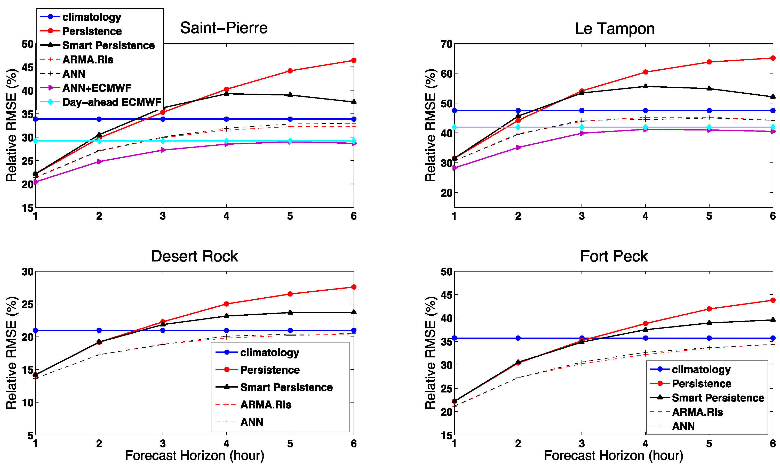
Second, regarding the rRMSE and rMAE metrics, Table 5 and Table 6, and Figure 7 show that the ANN and ARMA.RLS methods perform better than the reference models (Pers, Smart-pers and Climatology) for forecasting time horizons greater than one hour. Further, the gain in rRMSE or rMAE increases with the forecasting horizon.

Interestingly, Table 5 and Figure 7 show that the simple linear recursive ARMA.RLS model performs equally well than the nonlinear ANN model in terms of rRMSE. It even produces slightly better forecasts in the case of Saint-Pierre. However, in terms of rMAE, it appears that the ANN produces slightly better forecasts.

Table 4. rMBE values for the two insular sites. The corresponding MBE values can be obtained from the mean GHI of each site.

Site	Model	1 h Ahead	2 h Ahead	3 h Ahead	4 h Ahead	5 h Ahead	6 h Ahead
Le Tampon mean GHI: 427 W.m−2	Pers	2.1%	3.3%	3.5%	2.7%	0.7%	−1.8%
	Smart-Pers	2.1%	3.4%	2.3%	−0.6%	−3.1%	−3.5%
	Climatology	0.8%	0.8%	0.8%	0.8%	0.8%	0.8%
	ARMA.RLS	0.8%	0.4%	−0.4%	−1.2%	−1.0%	−1.0%
	ANN	0.7%	1.0%	0.4%	−0.1%	−0.3%	−0.1%
	ANN + ECMWF	−1.9%	−2.6%	−2.7%	−2.4%	−2.6%	−2.2%
Saint-Pierre mean GHI: 498 W.m−2	Pers	1.1%	0.9%	−0.3%	−2.3%	−4.3%	−5.9%
	Smart-Pers	1.1%	0.3%	−2.3%	−4.8%	−5.7%	−4.8%
	Climatology	−1.7%	−1.7%	−1.7%	−1.7%	−1.7%	−1.7%
	ARMA.RLS	−0.01%	−0.1%	−1.8%	−2.8%	−2.9%	−3.1%
	ANN	0.5%	0.06%	−0.5%	−1.2%	−1.5%	−1.8%
	ANN + ECMWF	0.2%	0.7%	0.8%	0.3%	−0.04%	−0.8%

Table 4. rMBE values for the two insular sites. The corresponding MBE values can be obtained from the mean GHI of each site.

Site	Model	1 h Ahead	2 h Ahead	3 h Ahead	4 h Ahead	5 h Ahead	6 h Ahead
Le Tampon mean GHI: 427 W.m−2	Pers	2.1%	3.3%	3.5%	2.7%	0.7%	−1.8%
	Smart-Pers	2.1%	3.4%	2.3%	−0.6%	−3.1%	−3.5%
	Climatology	0.8%	0.8%	0.8%	0.8%	0.8%	0.8%
	ARMA.RLS	0.8%	0.4%	−0.4%	−1.2%	−1.0%	−1.0%
	ANN	0.7%	1.0%	0.4%	−0.1%	−0.3%	−0.1%
	ANN + ECMWF	−1.9%	−2.6%	−2.7%	−2.4%	−2.6%	−2.2%
Saint-Pierre mean GHI: 498 W.m−2	Pers	1.1%	0.9%	−0.3%	−2.3%	−4.3%	−5.9%
	Smart-Pers	1.1%	0.3%	−2.3%	−4.8%	−5.7%	−4.8%
	Climatology	−1.7%	−1.7%	−1.7%	−1.7%	−1.7%	−1.7%
	ARMA.RLS	−0.01%	−0.1%	−1.8%	−2.8%	−2.9%	−3.1%
	ANN	0.5%	0.06%	−0.5%	−1.2%	−1.5%	−1.8%
	ANN + ECMWF	0.2%	0.7%	0.8%	0.3%	−0.04%	−0.8%

Table 5. rRMSE values for the three sites. The corresponding RMSE values can be obtained from the mean GHI of each site.

Site	Model	1 h Ahead	2 h Ahead	3 h Ahead	4 h Ahead	5 h Ahead	6 h Ahead
Le Tampo Mean GHI: 427 W.m−2	Pers	31.5%	44.2%	54.1%	60.4%	63.8%	65.1%
	Smart-Pers	31.5%	45.7%	53.4%	55.6%	54.9%	52.1%
	Climatology	47.5%	47.5%	47.5%	47.5%	47.5%	47.5%
	ARMA.RLS	30.7%	39.7%	43.9%	45.2%	45.3%	44.3%
	ANN	30.7%	39.5%	44.3%	44.4%	45.0%	44.2%
	ANN + ECMWF	28.3%	35.1%	39.9%	41.2%	41.0%	40.6%
Saint-Pierre mean GHI: 498 W.m−2	Pers	22.2%	29.8%	35.3%	40.2%	44.2%	46.4%
	Smart-Pers	22.2%	30.5%	36.3%	39.3%	39.0%	37.5%
	Climatology	33.9%	33.9%	33.9%	33.9%	33.9%	33.9%
	ARMA.RLS	21.3%	27.0%	29.9%	31.5%	32.3%	32.3%
	ANN	21.4%	27.1%	30.0%	31.9%	32.8%	33.0%
	ANN + ECMWF	20.4%	24.8%	27.2%	28.5%	29.0%	28.7%

Table 5. rRMSE values for the three sites. The corresponding RMSE values can be obtained from the mean GHI of each site.

Site	Model	1 h Ahead	2 h Ahead	3 h Ahead	4 h Ahead	5 h Ahead	6 h Ahead
Le Tampo Mean GHI: 427 W.m−2	Pers	31.5%	44.2%	54.1%	60.4%	63.8%	65.1%
	Smart-Pers	31.5%	45.7%	53.4%	55.6%	54.9%	52.1%
	Climatology	47.5%	47.5%	47.5%	47.5%	47.5%	47.5%
	ARMA.RLS	30.7%	39.7%	43.9%	45.2%	45.3%	44.3%
	ANN	30.7%	39.5%	44.3%	44.4%	45.0%	44.2%
	ANN + ECMWF	28.3%	35.1%	39.9%	41.2%	41.0%	40.6%
Saint-Pierre mean GHI: 498 W.m−2	Pers	22.2%	29.8%	35.3%	40.2%	44.2%	46.4%
	Smart-Pers	22.2%	30.5%	36.3%	39.3%	39.0%	37.5%
	Climatology	33.9%	33.9%	33.9%	33.9%	33.9%	33.9%
	ARMA.RLS	21.3%	27.0%	29.9%	31.5%	32.3%	32.3%
	ANN	21.4%	27.1%	30.0%	31.9%	32.8%	33.0%
	ANN + ECMWF	20.4%	24.8%	27.2%	28.5%	29.0%	28.7%

Table 6. rMAE values for the two sites. The corresponding MAE values can be obtained from the mean GHI of each site.

Site	Model	1 h Ahead	2 h Ahead	3 h Ahead	4 h Ahead	5 h Ahead	6 h Ahead
Le Tampon mean GHI: 427 W.m−2	Pers	21.5%	31.1%	38.1%	42.9%	45.8%	47.1%
	Smart-Pers	21.5%	32.7%	38.5%	40.7%	40.2%	37.8%
	Climatology	37.0%	37.0%	37.0%	37.0%	37.0%	37.0%
	ARMA.RLS	23.5%	30.8%	34.0%	35.2%	35.0%	34.0%
	ANN	23.4%	30.3%	34.1%	34.5%	34.7%	33.6%
	ANN + ECMWF	20.4%	26.1%	29.3%	30.0%	30.0%	29.7%
Saint-Pierre mean GHI: 498 W.m−2	Pers	13.6%	19.2%	23.4%	27.1%	29.8%	31.2%
	Smart-Pers	13.6%	20.2%	25.1%	27.3%	26.6%	24.9%
	Climatology	25.2%	25.2%	25.2%	25.2%	25.2%	25.2%
	ARMA.RLS	15.0%	20.0%	22.6%	23.7%	24.3%	24.7%
	ANN	15.1%	19.7%	22.0%	23.7%	24.3%	24.4%
	ANN + ECMWF	13.7%	16.9%	18.9%	19.8%	20.2%	20.1%

Table 6. rMAE values for the two sites. The corresponding MAE values can be obtained from the mean GHI of each site.

Site	Model	1 h Ahead	2 h Ahead	3 h Ahead	4 h Ahead	5 h Ahead	6 h Ahead
Le Tampon mean GHI: 427 W.m−2	Pers	21.5%	31.1%	38.1%	42.9%	45.8%	47.1%
	Smart-Pers	21.5%	32.7%	38.5%	40.7%	40.2%	37.8%
	Climatology	37.0%	37.0%	37.0%	37.0%	37.0%	37.0%
	ARMA.RLS	23.5%	30.8%	34.0%	35.2%	35.0%	34.0%
	ANN	23.4%	30.3%	34.1%	34.5%	34.7%	33.6%
	ANN + ECMWF	20.4%	26.1%	29.3%	30.0%	30.0%	29.7%
Saint-Pierre mean GHI: 498 W.m−2	Pers	13.6%	19.2%	23.4%	27.1%	29.8%	31.2%
	Smart-Pers	13.6%	20.2%	25.1%	27.3%	26.6%	24.9%
	Climatology	25.2%	25.2%	25.2%	25.2%	25.2%	25.2%
	ARMA.RLS	15.0%	20.0%	22.6%	23.7%	24.3%	24.7%
	ANN	15.1%	19.7%	22.0%	23.7%	24.3%	24.4%
	ANN + ECMWF	13.7%	16.9%	18.9%	19.8%	20.2%	20.1%

One may also notice (see Figure 7) that the performances of the linear ARMA.RLS and nonlinear ANN models tend towards that of the climatological mean. This behavior is consistent, as these methods tend to asymptotically model the mean of the data.

Figure 7. rRMSE values for each forecasting time horizon. Note that, regarding the different curves, the same legends are used for both Saint-Pierre and Le Tampon.

Figure 7. rRMSE values for each forecasting time horizon. Note that, regarding the different curves, the same legends are used for both Saint-Pierre and Le Tampon.

Table 7 lists the s-skill scores of the different forecasting techniques for each forecasting time horizon. As shown by Table 7, the s-skill scores of the methods increase with the forecasting time horizon. The proposed models (ARMA.RLS, ANN) exhibit positive scores and therefore perform better than the persistence model.

Table 7. s-Skill scores (in %) for the four sites.

Site	Model	1 h Ahead	2 h Ahead	3 h Ahead	4 h Ahead	5 h Ahead	6 h Ahead
Le Tampon	Smart-Pers	0.0	−3.5	1.3	7.9	14.0	19.8
	Climatology	−50.8	−7.4	12.2	21.4	25.6	27.0
	ARMA.RLS	2.4	10.2	18.8	25.2	29.0	31.8
	ANN	2.4	10.7	18.2	26.5	29.5	32.0
	ANN + ECMWF	10.3	20.6	26.2	31.8	35.7	37.6
Saint-Pierre	Smart-Pers	0.0	−2.3	−2.7	2.4	11.7	19.1
	Climatology	−52.8	−13.5	4.1	15.8	23.4	27.0
	ARMA.RLS	3.7	9.4	15.5	21.6	27.0	30.3
	ANN	3.3	9.1	15.0	20.7	25.8	28.9
	ANN + ECMWF	7.8	16.9	22.9	29.1	34.4	38.2
Desert Rock	Smart-Pers	0.0	−0.1	1.8	7.3	10.7	14.0
	Climatology	−47.9	−9.5	5.8	16.1	20.9	24.0
	ARMA.RLS	3.8	9.9	15.3	20.7	23.9	26.0
	ANN	3.7	10.0	15.5	19.7	23.1	25.8
Fort Peck	Smart-Pers	0.0	−0.4	0.8	−21.7	7.2	9.6
	Climatology	−60.8	−17.4	−1.6	−15.9	14.8	18.5
	ARMA.RLS	5.0	10.4	14.0	−4.5	19.9	21.2
	ANN	4.5	10.4	13.0	−6.0	19.7	21.5

Table 7. s-Skill scores (in %) for the four sites.

Site	Model	1 h Ahead	2 h Ahead	3 h Ahead	4 h Ahead	5 h Ahead	6 h Ahead
Le Tampon	Smart-Pers	0.0	−3.5	1.3	7.9	14.0	19.8
	Climatology	−50.8	−7.4	12.2	21.4	25.6	27.0
	ARMA.RLS	2.4	10.2	18.8	25.2	29.0	31.8
	ANN	2.4	10.7	18.2	26.5	29.5	32.0
	ANN + ECMWF	10.3	20.6	26.2	31.8	35.7	37.6
Saint-Pierre	Smart-Pers	0.0	−2.3	−2.7	2.4	11.7	19.1
	Climatology	−52.8	−13.5	4.1	15.8	23.4	27.0
	ARMA.RLS	3.7	9.4	15.5	21.6	27.0	30.3
	ANN	3.3	9.1	15.0	20.7	25.8	28.9
	ANN + ECMWF	7.8	16.9	22.9	29.1	34.4	38.2
Desert Rock	Smart-Pers	0.0	−0.1	1.8	7.3	10.7	14.0
	Climatology	−47.9	−9.5	5.8	16.1	20.9	24.0
	ARMA.RLS	3.8	9.9	15.3	20.7	23.9	26.0
	ANN	3.7	10.0	15.5	19.7	23.1	25.8
Fort Peck	Smart-Pers	0.0	−0.4	0.8	−21.7	7.2	9.6
	Climatology	−60.8	−17.4	−1.6	−15.9	14.8	18.5
	ARMA.RLS	5.0	10.4	14.0	−4.5	19.9	21.2
	ANN	4.5	10.4	13.0	−6.0	19.7	21.5

6.5.2. Impact of the Sky Conditions on the Forecasts Accuracy

This section aims at assessing the impact of the sky conditions on the forecasting performance of the different methods. Figure 7 plots the performance of the different models (except the ANN + ECMWF model for the sites of Desert Rock and Fort Peck). Let us recall that the site of Desert Rock experiences high occurrences of clear skies and possesses a low annual variability. Fort Peck exhibits a somewhat less but still high occurrence of clear sky conditions with an annual variability similar to that of Saint-Pierre.

The performance of the models is obviously the best for the site of Desert Rock. At the opposite, more variable sky conditions lead to worse forecasting performances (case of Le Tampon).

As mentioned above, the s-skill scores of the ARMA.RLS and ANN methods demonstrate that these techniques outperform the references models (Persistence and Climatology) whatever the site under study. In other words, we can argue that the ARMA.RLS and ANN models offer a significant improvement over Persistence and Climatology by an amount that is fairly independent of the sky conditions experienced by a site.

It is interesting to note that the sites of Saint-Pierre and Fort Peck, which exhibit almost the same variability and $k{t}^{*}$ distributions, display almost the same rRMSE values. At a first glance, one can conjecture a link between variability and forecastability. Some recent works [39,40] have shown that the type of climate and the associate cloud patterns have a profound impact in the forecasting performance. The authors of these works ([39,40]) also went further by proposing some metrics, which were related to solar variability to a priori assess the accuracy of solar forecasting models (i.e., to estimate the forecasting performance before any forecasts are produced). In addition, [17] showed increasing RMSE values with increasing variability.

6.5.3. Models with Exogenous Inputs Provided by ECMWF (ANN+ECMWF Model)

Table 4, Table 5 and Table 6 and Figure 7 clearly demonstrate the improvement (at each forecast horizon) of the forecasting accuracy obtained from the combination of day-ahead ECMWF forecasts with on-site measured irradiance. One may also notice that higher values of s-skill scores (Table 7) are obtained with the ANN+ECMWF model.

Figure 7 also confirms that the rRMSE values of the ANN+ECMWF model tend towards that of the initial day-ahead ECMWF forecasts for Le Tampon and Saint-Pierre when the forecast horizon increases. The proposed combination of different type of forecasting models through the use of an ANN may be a viable alternative to the standard linear combination of forecasting models currently implemented by the solar forecasting community.

7. Main Conclusions

This work proposed to evaluate the accuracy of day-ahead and intra-day forecasts in a particular insular context. Two sites of Réunion Island, which are geographically close, but with very different sky conditions, were chosen for the benchmarking exercise.

Day-ahead forecasts were provided by the ECMWF. Model output statistics (MOS) methods were applied in an attempt to refine the ECMWF forecasts. It was shown that, due to the small scale of the island, a technique like spatial averaging was inefficient for the case of insular sites like Saint-Pierre and Le Tampon.

As the original day-ahead forecasts were biased, a bias correction method based on two techniques was tested. While the MOS correction method led to a significant bias reduction, it appears that more work must be done in order to improve the results. For instance, future work may consist in finding systematic dependencies of the bias in dependence on new parameters that could better describe the meteorological situation.

Intraday solar forecasts (from 1 h to 6 h ahead) were produced by two statistical models: a simple linear technique with recursive estimation of the model’s parameters and a non-linear artificial neural network. A first experimental set-up that consists in using only past on-site irradiance measurements was proposed. It was shown that the proposed models clearly outperformed the reference models like persistence or smart persistence for forecasting horizon greater that 1h. Interestingly, it was found that a linear recursive technique like ARMA.RLS performed equally well or slightly better than a non-linear method such as an artificial neural network. This finding if confirmed may favor in the future the use of such linear recursive model for short-term solar forecasting. In addition, the recursive estimation of the model’s parameters makes the method very well suited to online forecasting.

The second experimental set-up proposed the combination of day-ahead ECMWF forecasts with past ground measurements. It was demonstrated that the incorporation of additional exogenous inputs into the ANN model clearly improved the accuracy of the intra-day forecasts.

A future and interesting step could be the comparison of the proposed methods with satellite-based forecasts produced by the cloud motion vector (CMV) technique in the case of an insular context.

Finally, preliminary results showed an impact of the sky conditions on the forecasting accuracy of the different methods. Insular sites like Le Tampon, which exhibits higher solar variability due to clouds that are formed locally, are prone to have the worse forecasting performance than less variable (continental or insular) sites.

References

- Lorenz, E.; Heinemann, D. Prediction of solar irradiance and photovoltaic power. In Comprehensive Renewable Energy; Sayigh, A., Ed.; Elsevier: Oxford, UK, 2012; pp. 239–292. [Google Scholar]
- Badosa, J.; Haeffelin, M.; Chepfer, H. Scales of spatial and temporal variation of solar irradiance on Reunion tropical island. Sol. Energy 2013, 88, 42–56. [Google Scholar] [CrossRef]
- Lorenz, E.; Hurka, J.; Heinemann, D.; Beyer, H.G. Irradiance forecasting for the power prediction of grid-connected photovoltaic systems. IEEE J. Sel. Top. App. Earth Obs. Remote Sens. 2009, 2, 2–10. [Google Scholar] [CrossRef]
- Pelland, S.; Galanis, G.; Kallos, G. Solar and photovoltaic forecasting through post-processing of the global environmental multiscale numerical weather prediction model: Solar and photovoltaic forecasting. Prog. Photovolt.: Res. Appl. 2013, 21, 284–296. [Google Scholar] [CrossRef]
- Mathiesen, P.; Kleissl, J. Evaluation of numerical weather prediction for intra-day solar forecasting in the continental United States. Sol. Energy 2011, 85, 967–977. [Google Scholar] [CrossRef]
- Kostylev, V.; Pavlovski, A. Solar power forecasting performance towards industry standards. In Proceedings of the 1st International Workshop on the Integration of Solar Power into Power Systems, Aarhus, Denmark, 24 October 2011.
- Hernández-Torres, D.; Bridier, L.; David, M.; Lauret, P.; Ardiale, T. Technico-economical analysis of a hybrid wave power-air compression storage system. Renew. Energy 2015, 74, 708–717. [Google Scholar] [CrossRef]
- Haessig, P.; Multon, B.; Ben Ahmed, H.; Lascaud, S.; Bondon, P. Energy storage sizing for wind power: Impact of the autocorrelation of day-ahead forecast errors: Energy storage sizing for wind power. Wind Energy 2015, 18, 43–57. [Google Scholar] [CrossRef] [Green Version]
- Perez, R.; Lorenz, E.; Pelland, S.; Beauharnois, M.; Van Knowe, G.; Hemker, K.; Heinemann, D.; Remund, J.; Müller, S.C.; Traunmüller, W.; et al. Comparison of numerical weather prediction solar irradiance forecasts in the US, Canada and Europe. Sol. Energy 2013, 94, 305–326. [Google Scholar] [CrossRef]
- Kühnert, J.; Lorenz, E.; Heinemann, D. Satellite-based irradiance and power forecasting for the German energy market. In Solar Energy Forecasting and Resource Assessment; Kleissl, J., Ed.; Academic Press: Oxford, UK, 2013; pp. 267–297. [Google Scholar]
- Perez, R.; Kivalov, S.; Schlemmer, J.; Hemker, K.; Renné, D.; Hoff, T.E. Validation of short and medium term operational solar radiation forecasts in the USA. Sol. Energy 2010, 84, 2161–2172. [Google Scholar] [CrossRef]
- Dambreville, R.; Blanc, P.; Chanussot, J.; Boldo, D. Very short term forecasting of the global horizontal irradiance using a spatio-temporal autoregressive model. Renew. Energy 2014, 72, 291–300. [Google Scholar] [CrossRef]
- Reikard, G. Predicting solar radiation at high resolutions: A comparison of time series forecasts. Sol. Energy 2009, 83, 342–349. [Google Scholar] [CrossRef]
- Lauret, P.; Voyant, C.; Soubdhan, T.; David, M.; Poggi, P. A benchmarking of machine learning techniques for solar radiation forecasting in an insular context. Sol. Energy 2015, 112, 446–457. [Google Scholar] [CrossRef]
- Marquez, R.; Coimbra, C.F.M. Forecasting of global and direct solar irradiance using stochastic learning methods, ground experiments and the NWS database. Sol. Energy 2011, 8, 746–756. [Google Scholar] [CrossRef]
- Mestre, G.; Ruano, A.; Duarte, H.; Silva, S.; Khosravani, H.; Pesteh, S.; Ferreira, P.; Horta, R. An intelligent weather station. Sensors 2015, 15, 31005–31022. [Google Scholar] [CrossRef] [PubMed]
- Sengupta, M.; Habte, A.; Kurtz, S.; Dobos, A.; Wilbert, S.; Lorenz, E.; Stoffel, T.; Renné, D.; Gueymard, C.; Myers, D.; et al. Best Practices Handbook for the Collection and Use of Solar Resource Data for Solar Energy Applications. Available online: http://www.nrel.gov/docs/fy15osti/63112.pdf (accessed on 14 December 2015).
- Maxwell, E.; Wilcox, S.; Rymes, M. Users Manual for SERI QC Software, Assessing the Quality of Solar Radiation Data; Report No. NREL-TP-463–5608; National Renewable Energy Laboratory: Golden, CO, USA, 1993.
- SURFRAD Network, Monitoring Surface Radiation in the Continental United States. Available online: http://www.esrl.noaa.gov/gmd/grad/surfrad/index.html (accessed on 12 December 2015).
- Bird, R.E.; Hulstrom, R.L. Simplified the Clear Sky Model for Direct and Diffuse Insolation on Horizontal Surfaces; Technical Report No. SERI/TR-642–761; Solar Energy Research Institute: Golden, CO, USA, 1981. [Google Scholar]
- Badescu, V.; Gueymard, C.A.; Cheval, S.; Oprea, C.; Baciu, M.; Dumitrescu, A.; Iacobescu, F.; Milos, I.; Rada, C. Accuracy analysis for fifty-four clear-sky solar radiation models using routine hourly global irradiance measurements in Romania. Renew. Energy 2013, 55, 85–103. [Google Scholar] [CrossRef]
- AERONET. Available online: http://aeronet.gsfc.nasa.gov/ (accessed on 7 December 2015).
- World Ozone Mapping. Available online: http://es-ee.tor.ec.gc.ca/e/ozone/ozoneworld.htm (accessed on 7 December 2015).
- Ineichen, P. Comparison of eight clear sky broadband models against 16 independent data banks. Sol. Energy 2006, 80, 468–478. [Google Scholar] [CrossRef]
- Cros, S.; Liandrat, O.; Sébastien, N.; Schmutz, N.; Voyant, C. Clear sky models assessment for an operational PV production forecasting solution. In Proceedings of the 28th European PV Solar Energy Conference, Paris, France, 30 September–4 October 2013.
- Reindl, D.T.; Beckman, W.A.; Duffie, J.A. Evaluation of hourly tilted surface radiation models. Sol. Energy 1990, 45, 9–17. [Google Scholar] [CrossRef]
- Hoff, T.E.; Perez, R. Modeling PV fleet output variability. Sol. Energy 2012, 86, 2177–2189. [Google Scholar] [CrossRef]
- David, M.; Ramahatana, F.H.; Liandrat, O. Spatial and temporal variability of PV output in an insular grid: Case of Reunion Island. In Proceedings of the ISES Solar World Congress, Cancùn, Mexico, 3–7 November 2013.
- Coimbra, C.F.M.; Kleissl, J.; Marquez, R. Overview of solar-forecasting methods and a metric for accuracy evaluation. In Solar Energy Forecasting and Resource Assessment; Kleissl, J., Ed.; Academic Press: Oxford, UK, 2013; pp. 171–194. [Google Scholar]
- Lauret, P.; Fock, E.; Mara, T.A. A node pruning algorithm based on the Fourier amplitude sensitivity test method. IEEE Trans. Neural Netw. 2006, 17, 273–293. [Google Scholar] [CrossRef] [PubMed]
- Lauret, P.; Fock, E.; Randrianarivony, R.N.; Manicom-Ramsamy, J.F. Bayesian neural network approach to short time load forecasting. Energy Convers. Manag. 2008, 49, 1156–1166. [Google Scholar] [CrossRef]
- Ferreira, P.M.; Gomes, J.M.; Martins, I.A.C.; Ruano, A.E. A neural network based intelligent predictive sensor for cloudiness, solar radiation, and air temperature. Sensors 2012, 12, 15750–15777. [Google Scholar] [CrossRef] [PubMed]
- Hornik, K.; Stinchcombe, M.; White, H. Multilayer feedforward networks are universal approximators. Neural Netw. 1989, 2, 359–366. [Google Scholar] [CrossRef]
- Pinson, P. Very short term probabilistic forecasting of wind power with generalized logit-normal distributions. J. R. Stat. Soc.: Ser. C 2012, 61, 555–576. [Google Scholar] [CrossRef]
- Bacher, P.; Madsen, H.; Nielsen, H.A. Online short-term solar power forecasting. Sol. Energy 2009, 83, 1772–1783. [Google Scholar] [CrossRef]
- Pinson, P.; Reikard, G.; Bidlot, J.R. Probabilistic forecasting of the wave energy flux. Appl. Energy 2012, 93, 364–370. [Google Scholar] [CrossRef]
- Chatfield, C. Time Series Analysis, An Introduction; Princeton University Press: Princeton, NJ, USA, 1994. [Google Scholar]
- Ljung, L.; Söderström, T. Theory and Practice of Recursive System Identification; MIT Press: Cambridge, MA, USA, 1983. [Google Scholar]
- Voyant, C.; Soubdhan, T.; Lauret, P.; David, D.; Muselli, M. Statistical parameters as a means to a priori assess the accuracy of solar forecasting models. Energy 2015, 90, 671–679. [Google Scholar] [CrossRef]
- Pedro, H.T.C.; Coimbra, C.F.M. Short-term irradiance forecastability for various solar micro-climates. Sol. Energy 2015, 122, 587–602. [Google Scholar] [CrossRef]
© 2016 by the authors; licensee MDPI, Basel, Switzerland. This article is an open access article distributed under the terms and conditions of the Creative Commons by Attribution (CC-BY) license (http://creativecommons.org/licenses/by/4.0/).