The Intermittency of Turbulence in Magneto-Hydodynamical Simulations and in the Cosmos

Abstract

Turbulent dissipation is a central issue in the star and galaxy formation process. Its fundamental property of space–time intermittency, well characterised in incompressible laboratory experiments, remains elusive in cosmic turbulence. Progress requires the combination of state-of-the-art modelling, numerical simulations and observations. The power of such a combination is illustrated here, where the statistical method intended to locate the extrema of velocity shears in a turbulent field, which are the signposts of intense dissipation extrema, is applied to numerical simulations of compressible magneto-hydrodynamical (MHD) turbulence dedicated to dissipation scales and to observations of a turbulent molecular cloud. We demonstrate that increments of several observables computed at the smallest lags can detect coherent structures of intense dissipation. We apply this statistical method to the observations of a turbulent molecular cloud close to the Sun in our galaxy and disclose a remarkable structure of extremely large velocity shear. At the location of the largest velocity shear, this structure is found to foster 10× more carbon monoxide molecules than standard diffuse molecular gas, an enrichment supported by models of non-equilibrium warm chemistry triggered by turbulent dissipation. In our simulations, we also compute structure functions of various synthetic observables and show that they verify Extended Self-Similarity. This allows us to compute their intermittency exponents, and we show how they constrain some properties of the underlying three-dimensional turbulence. The power of the combination of modelling and observations is also illustrated by the observations of the ${\mathrm{CH}}^{+}$ cation that provide unique quantitative information on the kinetic energy trail in the massive, multi-phase and turbulent circum-galactic medium of a galaxy group at redshift $z=2.8$.

1. Introduction

The unprecedented development of observational capabilities has revolutionised our knowledge of the cosmic history of star formation [1]. A consensus is emerging, on observational grounds, that the growth of galaxies in the early universe is largely governed by the conversion of massive gas reservoirs into stars over timescales as long as several Gyr, in apparent contradiction with the fast hierarchical merging imposed by dark matter (DM) structures [2]. This is one facet of the overcooling problem, also present in the local universe: the gas cools and forms stars too fast in simulations in comparison to observations. Theoretically, this problem is somewhat alleviated by stellar- or Active Galaxy Nuclei (AGN)-driven feedback [3].

Molecules, traditionally seen as the tracers of the truly cold universe in which stars form at temperatures considerably lower than the high temperatures reached by cosmological simulations, have unveiled a clue to solve the overcooling problem. An additional heating source—the dissipation of turbulence—is needed in cold interstellar matter (ISM) to explain its observed emission in the pure rotational lines of ${\mathrm{H}}_2$ and the presence of molecules with highly endoenergetic formation routes, such as ${\mathrm{CH}}^{+}$ (see the review by Hennebelle and Falgarone [4]). These observations, performed in diverse environments and at many scales, show that a major fraction of the gas internal energy is not dissipated at a high temperature but enters a multi-phasic turbulent cascade that dissipates radiatively at the low temperatures of the molecular gas. This unknown fraction is an uncharted link to the energetics of galaxy and star formation which must be explored to access the “relative importance of purely gravitational effects and of gas-dynamical effects involving dissipation and radiative cooling” stressed long ago by White and Rees [5]. This is why the intermittent dissipation of turbulent energy is key in the unravelling of the star and galaxy formation processes.

1.1. The Abyss between Cosmic Turbulence and Theory and Laboratory Experiments …

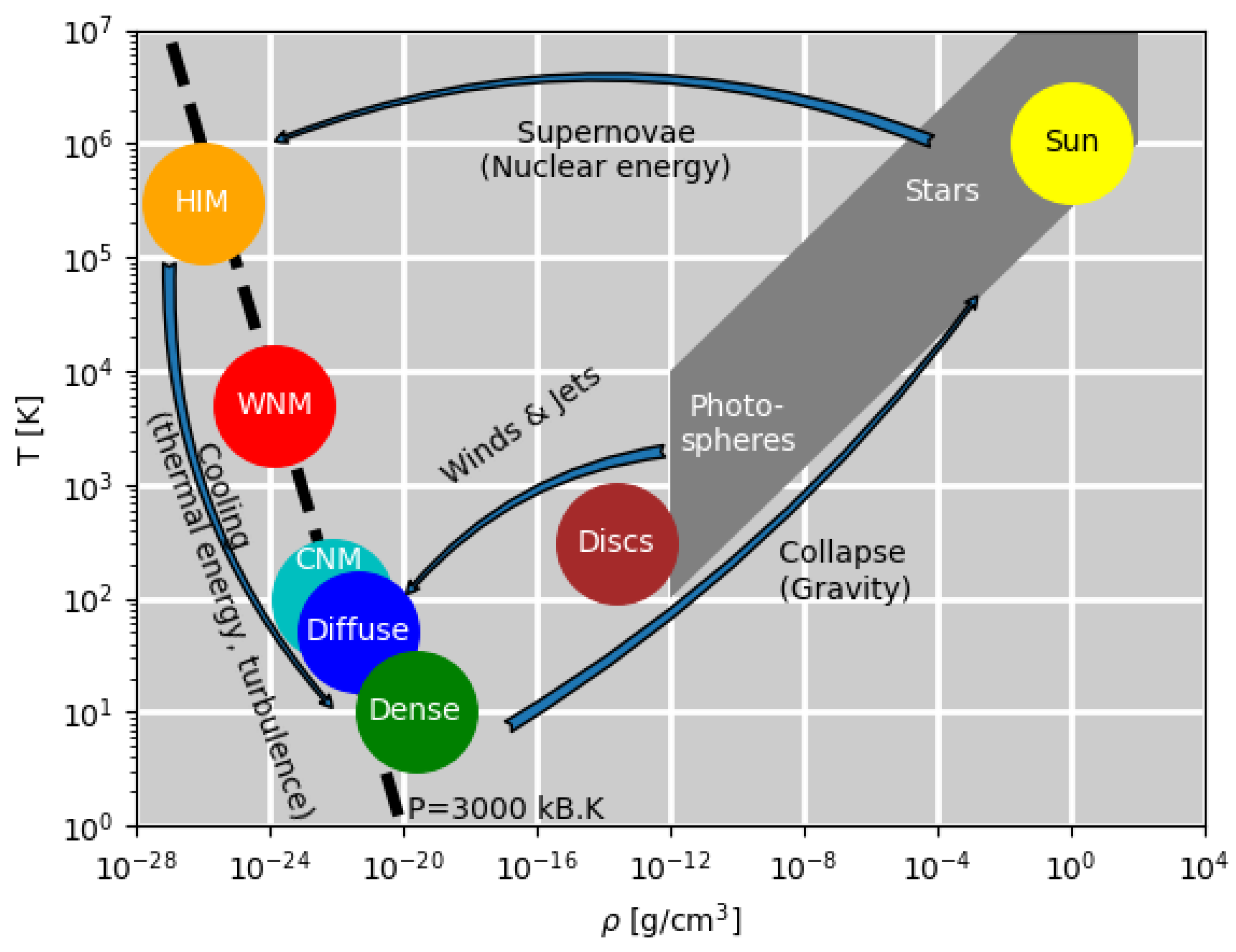
Theoretical approaches and experiments on isotropic, homogeneous, incompressible turbulence remain a powerful source of inspiration and guidance to the studies of the complex turbulence pervading space from the terrestrial atmosphere and solar wind to galaxies and galaxy clusters. To name a few in the scope of this paper: Chandrasekhar and Fermi [6] for the expression of the turbulent pressure and viscosity, Méneveau and Sreenivasan [7] and She and Lévêque [8] on space–time intermittency, Alexakis et al. [9,10] on non-local interactions in MHD turbulence, Moffatt et al. [11] for qualifying the coherent structures of vorticity as the sinews of turbulence, Uritsky et al. [12] for the similarity of the statistical properties of clusters of coherent structures of vorticity and current in MHD simulations, Kimura et al. [13] and Kimura and Sullivan [14] for the formation of strong temperature fronts in stably stratified turbulence, Cadot et al. [15] for imaging intense small-scale vortices in turbulent water seeded with gas bubbles, Tabeling et al. [16] for experiments in superfluid Helium, Politano and Pouquet [17] for their predictions of scaling laws in incompressible magnetised turbulence and Schekochihin [18] for clarifying the links between MHD and kinetic turbulence.

The applicability to cosmic turbulence of theoretical results obtained in idealised conditions is unexpected because cosmic turbulence is highly compressible, magnetised and multi-phasic with Reynolds numbers $Re=L{u}_{\mathrm{r}.\mathrm{m}.\mathrm{s}.}/\nu$ larger than ${10}^8$, where $L>100$ pc – two practical units for lengths/distances in astrophysics are the astronomical unit (au), the Earth–Sun distance, 1.5 × ${10}^{13}$ cm and the parsec (pc), 3 × ${10}^{18}$ cm, adapted to proto-planetary disks and galactic scales, respectively – and $u_{\mathrm{r}.\mathrm{m}.\mathrm{s}.}>10$ km s${ }^{-1}$ are the characteristic length and velocity of the integral scales of turbulence in galaxies and $\nu =\frac{1}{3}\lambda v_{\mathrm{th}}$∼${10}^{18}$ cm${ }^2$ s${ }^{-1}$, with $v_{\mathrm{th}}$ the thermal velocity, is the molecular viscosity. The colossal range of densities and temperatures experienced by the gas along its cycle between stars and the interstellar medium (ISM) is illustrated in Figure 1.

The CNM and WNM (Figure 1) are two thermally stable phases [19] that build up the so-called “cold” ISM, with respect to the hot space-filling phase. Their characteristics are given in Table 1. They are in thermal pressure equilibrium and their average densities (and temperatures) differ by about 2 orders of magnitude. The ISM therefore harbours gas structures about 100× denser and colder than their environment called “clouds”. The mass fraction in the dense phase depends on the ambient thermal pressure, and therefore on the distance from the stellar disks in galaxies. The ISM is fully or partially ionised depending on the ambient density of ionising ultra-violet (UV) photons and relativistic particles (cosmic rays, CR). The gas is therefore more or less coupled to the magnetic fields. The ISM also comprises sub-micron-size dust particles that contribute only 1% of the gas mass but play a key role in the gas coupling to the magnetic fields because these dust particles are charged and have a large collisional cross-section with the gas. They bear predominantly positive charges, except the smallest, which are predominantly negative [20], but their charge varies with the time and place depending on their environment (UV radiation and gas density).

Figure 1. Temperature–density cycle of baryonic matter from the various thermal phases of the interstellar medium (ISM), the stars themselves and its ejection back to the ISM through winds, jets and supernova explosions. The different thermal phases are the hot ionised medium (HIM), the warm neutral medium (WNM), the cold (atomic) neutral medium (CNM) and denser molecular phases, noted as diffuse and dense (see Table 1 for the characteristics of each of these thermal phases). The energy and processes driving the evolution along each branch of the cycle are indicated. Note that turbulence is an actor along the cooling branch on the left of the cycle and that all the thermal phases of the ISM, except the densest, which are gravitationally bound, are in thermal pressure equilibrium. (Figure adapted from Lesaffre [21]).

Figure 1. Temperature–density cycle of baryonic matter from the various thermal phases of the interstellar medium (ISM), the stars themselves and its ejection back to the ISM through winds, jets and supernova explosions. The different thermal phases are the hot ionised medium (HIM), the warm neutral medium (WNM), the cold (atomic) neutral medium (CNM) and denser molecular phases, noted as diffuse and dense (see Table 1 for the characteristics of each of these thermal phases). The energy and processes driving the evolution along each branch of the cycle are indicated. Note that turbulence is an actor along the cooling branch on the left of the cycle and that all the thermal phases of the ISM, except the densest, which are gravitationally bound, are in thermal pressure equilibrium. (Figure adapted from Lesaffre [21]).

Table 1. Characteristic scales and dimensionless numbers for various thermal phases in the galaxy, from the most dilute to the densest. HIM: hot ionised medium, WNM: warm neutral medium, CNM: cold neutral medium, diffuse and dense molecular gas. These characteristic values are orders of magnitude from Draine [22], (p.6, Table 1.3). Dimensionless numbers are defined as $\mathcal{M}=u_{\mathrm{r}.\mathrm{m}.\mathrm{s}.}/v_{\mathrm{th}}$, the Mach number; $Re=L{u}_{\mathrm{r}.\mathrm{m}.\mathrm{s}.}/\nu$ (see text), the Reynolds number; $Rm=L{u}_{\mathrm{r}.\mathrm{m}.\mathrm{s}.}/\eta$, the magnetic Reynolds number (the resistivity $\eta$ is computed as in Equation (12) of Balbus and Terquem [23]); and $R_{AD}=L/\left(u_{\mathrm{r}.\mathrm{m}.\mathrm{s}.}{t}_a\right)$ is a dimensionless number based on the ambipolar diffusion process (see Equation (3) of Momferratos et al. [24]), where $t_a$ is the ion-neutral momentum exchange time scale.

	HIM	WNM	CNM	Diffuse H${ }_2$	Dense H${ }_2$
Density n [cm${ }^{-3}$]	0.004	0.6	30	200	10${ }^4$
Temperature T [K]	3.10${ }^5$	5000	100	50	10
Length scale L [pc]	100	50	10	3	0.1
Velocity $u_{\mathrm{r}.\mathrm{m}.\mathrm{s}.}$ [km.s${ }^{-1}$]	10	10	10	3	0.1
$\mathcal{M}$	0.2	2	13	7	0.5
$Re$	10${ }^2$	10${ }^5$	10${ }^7$	10${ }^7$	10${ }^6$
$Rm$	10${ }^{21}$	10${ }^{20}$	10${ }^{18}$	10${ }^{17}$	10${ }^{15}$
$R_{AD}$	10${ }^3$	10${ }^3$	10${ }^2$	10${ }^3$	10${ }^4$
Ionisation fraction	1	10${ }^{-2}$	10${ }^{-4}$	10${ }^{-4}$	10${ }^{-7}$

Table 1. Characteristic scales and dimensionless numbers for various thermal phases in the galaxy, from the most dilute to the densest. HIM: hot ionised medium, WNM: warm neutral medium, CNM: cold neutral medium, diffuse and dense molecular gas. These characteristic values are orders of magnitude from Draine [22], (p.6, Table 1.3). Dimensionless numbers are defined as $\mathcal{M}=u_{\mathrm{r}.\mathrm{m}.\mathrm{s}.}/v_{\mathrm{th}}$, the Mach number; $Re=L{u}_{\mathrm{r}.\mathrm{m}.\mathrm{s}.}/\nu$ (see text), the Reynolds number; $Rm=L{u}_{\mathrm{r}.\mathrm{m}.\mathrm{s}.}/\eta$, the magnetic Reynolds number (the resistivity $\eta$ is computed as in Equation (12) of Balbus and Terquem [23]); and $R_{AD}=L/\left(u_{\mathrm{r}.\mathrm{m}.\mathrm{s}.}{t}_a\right)$ is a dimensionless number based on the ambipolar diffusion process (see Equation (3) of Momferratos et al. [24]), where $t_a$ is the ion-neutral momentum exchange time scale.

	HIM	WNM	CNM	Diffuse H${ }_2$	Dense H${ }_2$
Density n [cm${ }^{-3}$]	0.004	0.6	30	200	10${ }^4$
Temperature T [K]	3.10${ }^5$	5000	100	50	10
Length scale L [pc]	100	50	10	3	0.1
Velocity $u_{\mathrm{r}.\mathrm{m}.\mathrm{s}.}$ [km.s${ }^{-1}$]	10	10	10	3	0.1
$\mathcal{M}$	0.2	2	13	7	0.5
$Re$	10${ }^2$	10${ }^5$	10${ }^7$	10${ }^7$	10${ }^6$
$Rm$	10${ }^{21}$	10${ }^{20}$	10${ }^{18}$	10${ }^{17}$	10${ }^{15}$
$R_{AD}$	10${ }^3$	10${ }^3$	10${ }^2$	10${ }^3$	10${ }^4$
Ionisation fraction	1	10${ }^{-2}$	10${ }^{-4}$	10${ }^{-4}$	10${ }^{-7}$

Turbulence is ubiquitous throughout this cycle. Its origins are multiple, including the differential rotation of galaxies, the gravitational energy in gas accretion processes and the stellar feedback in the form of supernova explosions but also jets and winds all along the stellar lifetime that span several Gyr for solar-type stars. The role of turbulence in star formation, in particular, its link with the observed very low efficiency of star formation, is a highly debated issue because turbulence can both trigger and hamper star formation (see the review by Hennebelle and Falgarone [4]).

The large scales in cosmic turbulence concern rotating and shearing, stratified by the gravitation field, with an additional anisotropy due to the ubiquitous magnetic fields. The associated dynamical timescales are all different and span a broad range from hundreds of Myr to ∼${10}^3$ yr. The latter are shorter than collisional times, providing the ISM with facets of collisionless plasma (see the review by Ferrière [25]). A fraction of the cold medium lies in the thermally unstable phase because turbulence continuously drives the phase transition from the WNM to CNM [26]: the hydrodynamic pressure fluctuations of the turbulence destabilise the WNM and cause its fragmentation into CNM clouds, harboring droplets as dense as ${10}^4$${\mathrm{cm}}^{-3}$. Buoyancy in the galactic gravitational field is also inevitable given the gas equation of state and the multiplicity of energy and ionisation sources.

Finally, the weakly ionised ISM phases are not fully coupled to the magnetic fields. There is a whole range of high frequencies of magnetic waves which are not perceived by the plasma because the collisions of neutrals with ions and charged dust grains, closely coupled to the magnetic fields, are too rare. There is also a domain, at low frequency, where the waves no longer propagate because all their energy is dissipated in ion-neutral collisions. The frequencies that limit these regimes depend on the collision cross-sections between the ions and the neutrals and their respective densities [27]. Between these two extremes, the magnetic fields drift through the medium. This is an important phenomenon in the diffuse ISM because it is a major source of energy dissipation but it is also the reason that C-shocks (i.e., continuous shocks) exist, because, unlike J-shocks, they develop magnetic precursors [28,29,30]. This is also why they are so rich in molecules.

1.2. …and yet

In spite of all the above, the electron density of the ISM and interplanetary ionised medium exhibits a Kolmogorov power spectrum spanning more than 10 orders of magnitude in scales down to ∼${10}^8$ cm (known as “The big power law in the sky”) [31]. The slope of this spectrum suggests a link with turbulence.

Cold atomic gas too exhibits a structure down to very small scales of 10 to ${10}^4$ au [32]. A few power spectra have been observed in the CNM: that of the continuum emission of dust in a high-galactic-latitude cloud extending from 20 pc down to 2000 au [33], that of light scattered by dust in a similar field extending over 3 orders of magnitude down to 10 mpc [34]. Both are consistent with the Kolmogorov spectrum, given the projection effects in observations (see next section).

The molecular component of the CNM (hereafter molecular clouds) also exhibits power law scalings between the velocity dispersion and size scale, the well-known linewidth-size relations of Larson [35], and is now observed in many environments including external galaxies (e.g., [4,36]) with a range of slope values close, but not equal, to the Kolmogorov spectrum. An extension of the Kolmogorov cascade, taking into account compressibility, has been proposed by Kritsuk et al. [37] using a density-weighted velocity $\mathbf{v}={\rho }^{1/3}\mathbf{u}$ with $\rho$ as the mass density; this preserves the Kolmogorov scaling of the power spectra and the third-order structure-function behaviour. But the respective roles of self-gravity and turbulence in these linewidth-size scalings remain an outstanding issue (e.g., [38]).

Diffuse molecular gas (Figure 1) is responsible for the very first steps of chemistry in space with the formation of light hydrides, such as CH, OH, ${\mathrm{CH}}^{+}$, ${\mathrm{OH}}^{+}$, …, the most simple molecules that are the building blocks of the complex species found in dense proto-stellar cores or proto-planetary discs. It is in that diffuse medium of density $n_{\mathrm{H}}$∼$10-100$ ${\mathrm{cm}}^{-3}$ that the turbulent dissipation scale, estimated as $l_{\mathrm{diss}}={({\nu }^3/ϵ)}^{1/4}$ with the spatially averaged kinetic energy transfer rate $ϵ\approx 2\times {10}^{-25}$ $\mathrm{erg}{\mathrm{cm}}^{-3}{\mathrm{s}}^{-1}$ inferred from observations [4,39] is of the same order as the mean free path of atoms, or $\lambda$∼$l_{\mathrm{diss}}$∼2–10 au. It is therefore predictable that turbulent dissipation plays a key role in the very first steps of chemistry in space.

1.3. Specific Molecules As Tracers of Turbulent Dissipation

The emergence of molecules in the diffuse ISM raises outstanding issues: the observed abundances of the CO molecule in the diffuse molecular gas are an order of magnitude larger than what the chemistry driven by the UV photons and cosmic rays is able to produce (e.g., [40]). This problem emerged in fact in the 1940s with the discovery of the first molecules in diffuse medium, CH, CH${ }^{+}$ and CN, the formation of CH${ }^{+}$ being extremely endothermic. Energy inputs from stellar UV photons and cosmic rays are not sufficient to reproduce the observed column densities of these species. The same problem appeared later for HCO${ }^{+}$ (e.g., [41]) and for CO. Another major power source was needed. Several processes have been proposed, such as thermal conduction and turbulent transport [42] at the WNM/CNM interfaces or extreme dissipative events in interstellar turbulence, such as C-shocks [12,24,28,29,43,44,45,46,47,48,49,50,51,52,53,54,55], magnetised Burgers vortices [40]. The former two inject the thermal energy of the WNM into the CNM, while the latter feeds the chemistry with the turbulent energy of the CNM, which is an order of magnitude larger than its thermal energy, but is comparable to the thermal energy of the WNM. Ion-neutral drift in Alfvén waves have also been considered [44]. It is likely that they all contribute to exemplifying the tight coupling between the thermal and turbulent facets of ISM physics.

In situ measurements in the ISM are impossible and the measured quantities suffer projection effects. Velocities are measured via the Doppler effect of spectral lines so that only line-of-sight (los) velocities are accessible. Furthermore, the detected signal (i.e., a spectral line) is the line emission integrated along the whole line of sight: radiative transfer is therefore involved in the data interpretation. Displacements are inferred from distances projected in the plane of the sky (pos), so that only the pos variations of the los-integrated velocity are accessible, providing a proxy for the pos vorticity projection. Kinetic helicity cannot be directly measured. Only the intensity of the magnetic field los projection is accessible via the Zeeman effect [45] and the field direction, pos projected, is provided by polarisation measurements in different wavelength ranges (see the review by Ferrière [25]).

This is why, like luminescent plankton that shines in the spots of intense velocity shear in the breaking waves of tropical seas, molecules with highly endothermic formation rates are used as the tracers of dissipation bursts in cosmic turbulence. These specific molecules in diffuse molecular gas are therefore not only the tracers of extreme dissipation events in cosmic turbulence but also of the signposts of coherent structures that may be the seeds of more massive structures in molecular clouds, grown through braiding and coalescing [47]. Note that the extrema of current and vorticity in MHD turbulence are not randomly distributed in space and time but cluster in structures qualified as coherent because, following Moisy and Jiménez [46], their “inertial-range extent, implies a large-scale organization of the small-scale intermittent structures”.

This paper reports on numerical simulations of compressible MHD turbulence, dedicated to dissipation scales, performed to characterise the nature of the coherent structures in ISM turbulence where dissipation is concentrated [48] and to illustrate the statistics performed on synthetic observations to disclose such Coherent Structures of Intense Dissipation Extrema—hereafter called CSIDE—in diffuse molecular gas. Then, the first example of such a statistical study in a nearby diffuse molecular cloud is presented. A long and thin parsec-scale coherent structure of intense velocity shear is identified [49,50]. High-angular resolution observations disclose an even more intense velocity shear within it, on linear scales of only a few mpc. Last, the power of the so-called “warm chemistry” triggered by turbulent dissipation [40] is illustrated by observations in the circum-galactic medium of a starburst galaxy group at redshift $z=2.8$ [51].

2. Intermittency in Simulations of Magnetised Turbulence

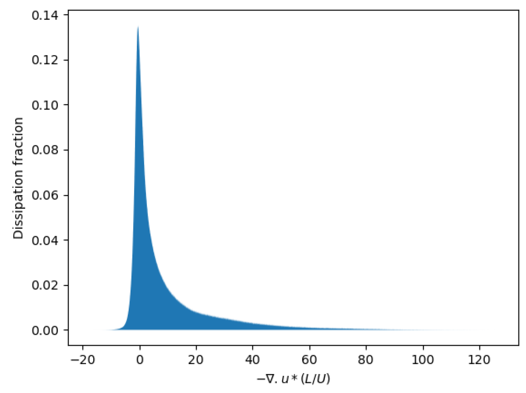
2.1. Numerical Dissipation

Coherent structures that are the signposts of intermittency [11,12,15,18,46] are hard to characterise in controlled laboratory experiments because measurements can only be made at a small finite number of points. On the contrary, a numerical simulation allows its user to access every state variable at every position. Unfortunately, that advantage comes with distortion from the unavoidable discretisation artefacts, and the inability to perform simulations at Reynolds numbers as large as in the experiments.

Simulations of incompressible gases allow one to compute gradients in Fourier space. Such techniques (“pseudo-spectral”) can obtain exponentially good accuracy with respect to the number of resolution elements. This greatly helps in trusting the dissipation terms when the resolution is large enough (i.e., when a bottleneck effect is absent). If the maximum wavenumber times the Kolmogorov dissipation scale is too small (lower than order unity, for example), Gibbs phenomena generate an excessive pile up of energy at small scales (i.e., the bottleneck effect). An exponential decay of power spectra at small scales is a good indication that numerical convergence has been obtained.The results of such incompressible simulations for hydrodynamical (HD) turbulence [46] show that dissipation is localised around vortices, and for MHD turbulence [12,24], they show that viscous and resistive dissipation are well separated on sheets which can therefore easily be identified as shearing or current sheets.

Compressible simulations are much more difficult to interpret. The finite size of the mesh and the necessary reconstruction of variables from the center to the edges of each pixel introduces a spurious diffusion length scale for every conservation equation (including mass conservation). To this effect, we built a method to estimate locally the total dissipation including the one inherent to the numerical scheme [24,48]. The method consists of replaying a simulation step while integrating a redundant conservation equation for a variant of the energy (total mechanical energy, for example). In isothermal simulations, that quantity is best taken as the generalised isothermal total mechanical energy $E=\frac{1}{2}\rho u^2+\frac{1}{8\pi }B+plog\rho$, where $\rho$, u, B and $p=\rho c_{\mathrm{s}}^2$ are, respectively, the mass density, the velocity, the magnetic field intensity and the thermal pressure (with $c_{\mathrm{s}}$ as the isothermal sound speed). An estimation of the flux ${\mathcal{F}}_E$ of this quantity and its time derivative then allows one to recover the local total dissipation of energy as $\epsilon ={\partial }_{t}E+\nabla .{\mathcal{F}}_E$.

Once the dissipation rate is known everywhere, we can study the regions of most intense dissipation. For instance, we can plot the los-integrated dissipation as on Figure 2: the regions of highest dissipation are not randomly distributed in space, they display large-scale and thin ridges of intense integrated dissipation. These ridges appear as a caustic effect from the projection of sheets seen almost edge-on where dissipation is intense (see [48]). They are coherent large-scale structures, hereafter called the CSIDE, as opposed to quasi-thermalized small-scale eddies.

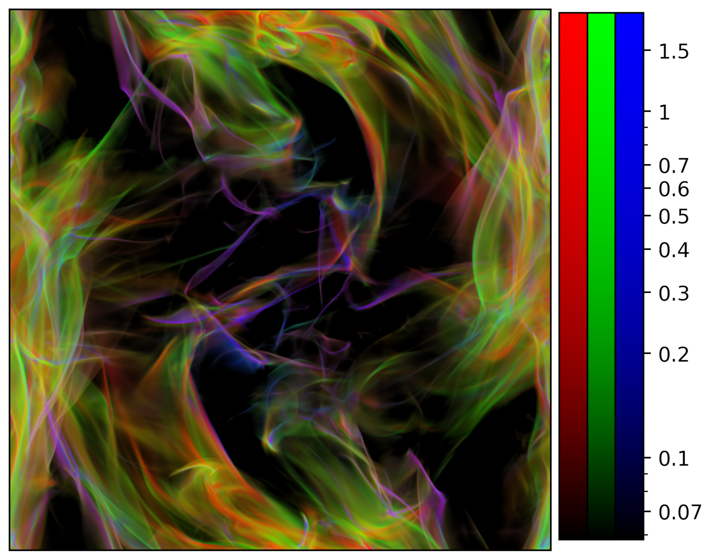
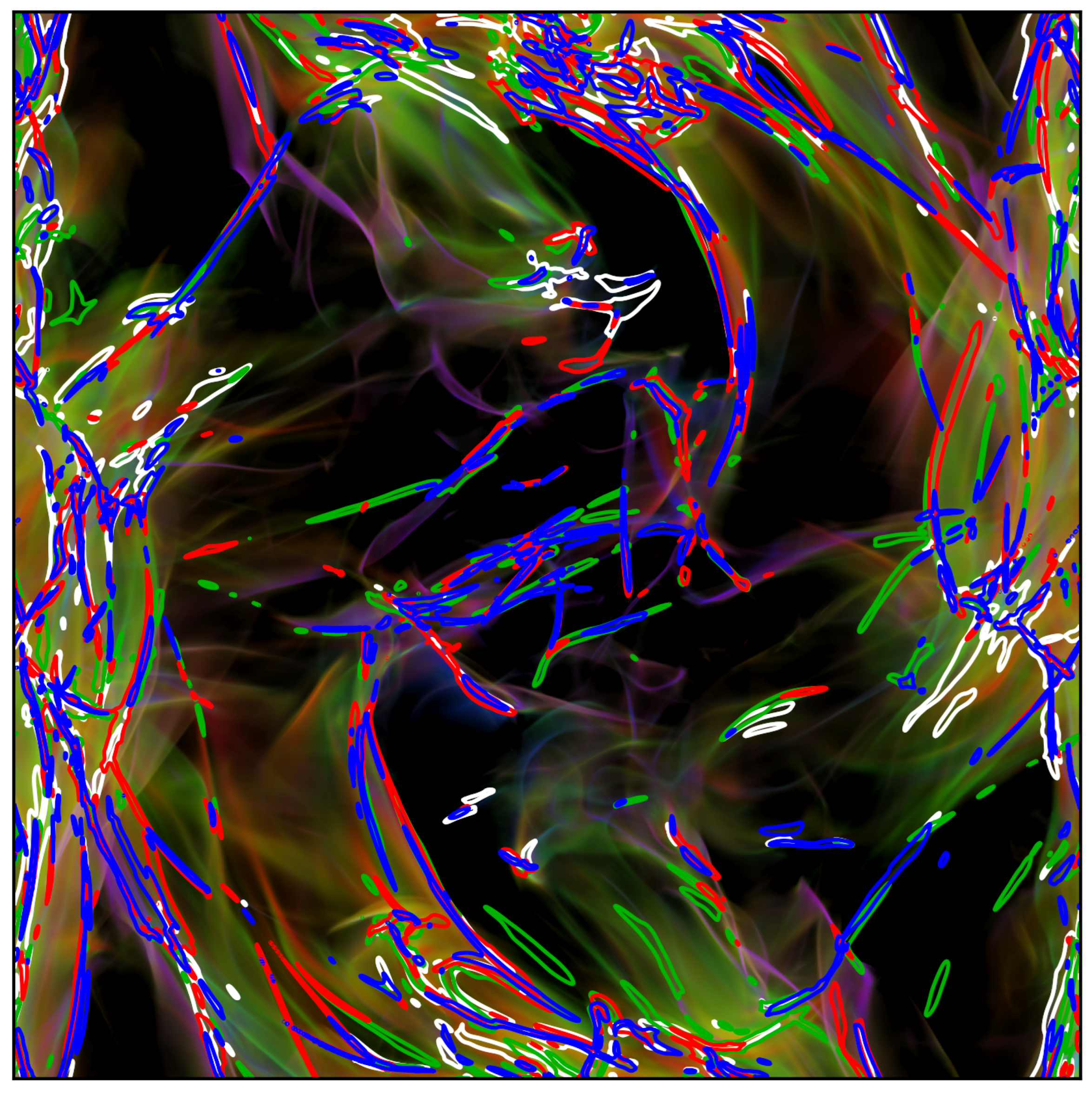
2.2. The Nature of Coherent Structures in MHD Turbulence

Intense dissipation in MHD turbulence is therefore seen to lie on thin sheets whether it is incompressible [12,24] or compressible [48]. In incompressible MHD turbulence, viscous and ohmic dissipation always appear disconnected (e.g., [12,24]), and the same probably holds for reduced MHD, as in [52]. In these works, it makes it easy to differentiate shearing sheets and current sheets as connected sets of intense viscous or resistive dissipation.

In compressible MHD turbulence, this is much less obvious, as hinted at in Figure 2, where different natures of dissipation heating can be intermixed. Lehmann et al. [53], with the SHOCKFIND algorithm, and Richard et al. [48] designed several criteria which allow one to carefully select strong dissipation regions and characterise their physical nature as fast shocks, slow shocks, rotational discontinuities or Parker sheets. Some of these criteria are based on Rankine–Hugoniot relations [54], which seem to hold strikingly well far from their domain of application (i.e., in a non-stationary medium, inhomogeneous, with curved working surfaces, etc.). Some of these criteria are based on decomposition along free travelling waves, which characterise suprisingly well most of these structures. Gradients of fast, intermediate and slow waves form an orthogonal basis of gradients of MHD variables. It turns out that slow shocks decompose almost purely on gradients of slow waves, and similarly, fast shocks on fast waves.

A systematic investigation of these CSIDE was performed by Richard et al. [48] for three-dimensional (3D) MHD turbulence and in Lesaffre et al. [55] for two-dimensional (2D) HD turbulence. For 2D HD, we were able to show that almost 80% of the dissipation was accounted for near the shock fronts, with the remainder as diffuse viscous shear in the wakes of these shocks [55]. In this setup, the effect of dissipation on the chemistry of the medium was to enhance the formation of molecules such as CH${ }^{+}$ or CO and collisionally excite H${ }_2$ molecules. For 3D MHD turbulence [48], we could not clearly prove whether there was a significant contribution from dissipation outside the detected CSIDE, given the technical difficulties introduced by the 3D geometry, but we computed that up to 30% of the dissipation occurs in less than 1% of the volume. We were surprised as most of the dissipation was accounted for by weakly compressive structures. This is illustrated by the distribution of the dissipation rate according to velocity convergence in Figure 3. Another surprise we found in Richard et al. [48] is that the entrance parameters in the Rankine–Hugoniot fronts we extract from the simulations do not span the whole parameter space available to them. Indeed, geometry and symmetries alone allow one to reduce to three the number of free parameters characterising a Rankine–Hugoniot discontinuity [54]. However, the dynamics of these dissipative structures seem to constrain them to lie on a two-dimensional parameter space. To be more precise, slow shocks and Alfvénic discontinuities have entrance magnetic fields nearly orthogonal to the discontinuity while fast shocks have their entrance magnetic fields nearly transverse. It will be the object of future investigations to understand the underlying reasons as to why this is.

2.3. Synthetic Observables and the CSIDE

Laboratory measurements or in situ probes borne by satellites in the Solar Wind (e.g., [56]) allow one to probe only a small fraction of the volume of interest. In experiments, the progress of particle image velocimetry (PIV) techniques now authorise somewhat more widespread measurements, and Cadot et al. [15] cleverly used cavitation bubbles to reveal the most intense coherent structures in their experiments. On the other hand, astrophysical images of the nearby interstellar medium offer a global view, however they are projected on the pos: we lose one dimension of interest, and radiative transfer effects as well as chemical and line excitation issues conspire to distort the los integration process. Nevertheless, some distinctive features survive the projection. Figure 2 suggests that when viewed sideways, CSIDE can still be seen as prominent features in the integrated image.

Here, we compute some proxies for los-integrated observable variables in our isothermal simulations of decaying MHD turbulence (see [48] for a detailed presentation of the simulations), and we investigate where they vary strongly. The first obvious quantity we have access to is the column density $I={\int }_0^L\rho dz$ (where L is the box length and z is the line of sight coordinate), probed indirectly by the intensity of the dust thermal continuum emission. Thanks to line profile measurements (see Section 4), one has access to a proxy of a density-weighted average los velocity $v_z={\int }_0^L\rho u_{z}dz/I$, provided one finds a trustable tracer of density. In practice, temperature and chemical effects due to local heating as well as radiative transfer effects strongly hinder this measurement (see Section 3 and Section 4). Finally, as the medium is magnetised, dust thermal emission is polarised. Modern astronomical instruments are able to measure the polarisation state of this emission, which is characterised through the Stokes parameters Q and U. The observed Stokes parameters are thus probes, however rather convoluted because polarisation is a pseudo-vector, of the los-integrated magnetic field direction. The polarisation of the dust thermal emission is due to the fact that dust grains are elongated and spin with their longer axis perpendicular to the magnetic field direction, thus orienting the polarisation vector of their thermal emission orthogonal to the magnetic field direction. The resulting Stokes parameters of dust emission, as computed in the numerical simulations, are therefore $Q+iU={\int }_0^{L}dz\rho {\widehat{B}}_{\perp }^2{e}^{2i\varphi }$, where $\varphi$ is the position angle of the magnetic fields on the plane of sky and ${\widehat{B}}_{\perp }$ is its relative norm compared to the local total fields.

In order to emphasise the locations where these observables change abruptly, we compute their one-pixel increments on the plane of the sky: i.e., around each pixel, we compute the standard deviation of the difference with its nearest neighbours. We then overlay 2-$\sigma$ contours of these increments onto our integrated dissipation map (see Figure 4). In most cases, such contours delimit a region of strong dissipation. Indeed, whenever a physical quantity varies strongly, it is most often associated with dissipation. However, not all dissipation regions are detected, and various observables highlight different parts of the regions, depending on which component of the velocity or the magnetic fields is probed by the observable considered. Indeed, some dissipation regions can involve a jump in magnetic fields or velocity components which cannot be probed by astrophysical observables because of the projections discussed in Section 1. Unfortunately, we are not yet in a capacity to link the nature of the observable jumps to the nature of the underlying dissipative structure, except for the simple fact that strongly compressive shocks (slow shocks) should appear as a ridge of strong $\delta I$ when their working surface contains the line of sight. But since the increments of synthetic observables provide a method to pinpoint and map CSIDE, these structures will be located in cosmic turbulence following this method, and further observed (e.g., at higher angular resolution, or with different observables) and the results of these additional observations will help us in understanding the nature of cosmic turbulence.

2.4. Intermittency Statistics from Increments of Observables

Since the early works of Kolmogorov [57] (K41), who predicted it in the case of incompressible hydrodynamics, one of the first characteristics of turbulence that researchers have strived to predict is the power law slope of the velocity power spectrum. In the case of incompressible MHD turbulence, the exact scaling laws of the velocity and magnetic fields are still a matter of debate [18,58,59,60]. In compressible turbulence, theoretical discussions are scarce, but suggest that one could obtain the K41 scaling for ${\rho }^{1/3}u$ in isothermal turbulence [61], while numerical simulations [62] display different scalings for subsonic (K41) and supersonic scales (Burgers). Banerjee and Galtier [63] also managed to derive exact expressions for convoluted transfer functions in isothermal MHD, from which it is, however, hard to derive scaling laws for any simply defined quantity. The power spectrum of the density and the column density have also been discussed and either proven to be K41 in the Gaussian case [64], or shown to be close to K41 thanks to numerical simulations [65,66].

Twenty years after K41, Kolmogorov [67] realised that the spatial intermittency of the dissipation rate would introduce corrections to the structure function power law scalings with lag (the so-called anomalous scalings, characterised by intermittency exponents or multifractal spectra [68]). These anomalous scalings were linked to the fractal dimension of the dissipative structures, and generic models such as that of She and Leveque [8] were put in place, with shape parameters for the fractal geometry of the dissipative structures. Based on the observation that these were sheets in the case of MHD turbulence, this led to independent predictions from Grauer et al. [69] and Politano and Pouquet [70] for the Iroshnikov–Kraichnan scaling and later from Boldyrev et al. [71] for the Goldreich–Sridhar scaling (similar to K41).

Note that the causal link between the geometry of the coherent structures and the form of the intermittency exponents goes only one way. For instance, random fields built with controlled anomalous scalings close to those of hydrodynamics [72] or MHD [73] do not display any coherent structures. It is only in the case where a statistical collection of well-defined structures of strong dissipation is presupposed that the anomalous scaling coefficients can constrain the fractal dimension and geometry of these structures.

In the previous section, we demonstrated a spatial link between the increments of the synthetic observables and the CSIDE. We now investigate these increments at various lags, and look at classical structure functions built from these increments. Even though these indicators are very indirect and probably have not much to do with the underlying physics of the above intermittent theoretical models, we proceed to compute them as they will presumably still be good probes of the relative orientation and size of the salient features in the astrophysical images (they will be sensitive to their fractal structure, for example). As such, they provide a quantitative estimate to link the texture of the simulated images to the observed ones. In addition, the link to physics is blurred by the projections, and this analysis should rather be regarded as a quantitative characterisation of the evolution of the observable increments statistics with scale.

We now define ${\delta }_{\ell }X\left(\mathit{r}\right)=X(\mathit{r}+\ell )-X\left(\mathit{r}\right)$ as the increment of an integrated observable X over a lag ℓ at position $\mathit{r}$ in the plane of sky and we investigate the statistics of these increments for lags where the norm is comprised between ℓ and $\ell +1$ pixels (hence, we compute all increments in a corona of a width of 1 pixel around each pixel).

Figure 5, for example, shows how the probability distribution function (PDF) of the increment of the los-integrated velocity ($v_z$) varies from having strong non-Gaussian wings at small scales to being nearly Gaussian at large scales. As an illustration, the interior of the green contours of Figure 4 corresponds to the wings of the PDF for the smallest lag (dark blue on Figure 3), where the normalised increment $\delta v_z/\sigma \left(\delta v_z\right)$ exceeds 2 in its absolute value.

We then define “structure functions” in a natural way similarly to three-dimensional dynamically relevant structure functions: $S(p,\ell )=<|{\delta }_{\ell }{X|}^p{>}_{\ell \le \left|\ell \right|<\ell +1}$, where the average is presented over the image. These are displayed in Figure 6, left panel. We now measure scaling exponents ${\zeta }_p$ by adjusting a power law $S(p,\ell )$∼${\ell }^{{\zeta }_p}$ in a range of scales ${\ell }_{min}\le \ell \le {\ell }_{max}$. We adopt here the range of scales for the lags between 12 and 48 pixels (over a periodic computational domain of 1024 pixels aside) as this seems to minimise the dispersion (see Figure 6 left panel).

The values of the scalings, displayed on the left panel of Figure 7, usually fall way above K41: even if we would fit a slope to the values of ${\zeta }_p$ vs p, we would find slopes much larger than K41 or Iroshnikov–Kraichnan: we are clearly not in the domain of the application of these theories. Furthermore, all exponents measured on different variables (column density, projected velocity, U and Q Stokes parameters) display anomalous scalings in the sense that ${\zeta }_p$ is not proportional to p (see Figure 7). The uncertainty of the fit is displayed as error bars of one standard deviation around these intermittency exponents. It is a quantitative measurement of whether the scaling is indeed good or not, i.e., whether intermittency exponents are a good representation of the data. Note that these error bars do not reflect the temporal variation in the simulation, as they are displayed here only for one selected snapshot (at a time close to the dissipation peak, about a third of the non-linear initial turnover time). The temporal variability of these coefficients is in fact a few times larger than the displayed error bars.

Figure 6 demonstrates that when we plot the structure functions against $S(3,\ell )$ instead of the lag (right panel vs left panel), they behave much more like power laws. This was first discovered by Benzi et al. [74] for three-dimensional velocity field increments in hydrodynamics experiments. Because this allowed one to significantly extend the range of the scaling, this property was named “Extended Self-Similarity” (ESS). Similarly, we define ESS exponents as the exponents in the power law scalings $S(p,\ell )$∼$S{(3,\ell )}^{\mathrm{ESS}{\zeta }_p}$. This significantly improves the quality of the fit, hence, our error bars (see right panel of Figure 7), even though we now use the full range of scales instead of the small restricted range of scales used in the left panel. This ESS property has been tested and verified in many independent data but has yet to find an underlying physical interpretation or proof. In addition, in our astrophysical case, for the observables integrated on the line of sight, the notion of an inertial range is hard to characterise. Indeed, projection brings larger scales onto smaller ones, and in doing so mixes dissipation, injection and inertial scales: this ESS property comes even more as a surprise.

We have investigated two types of initial conditions (an Arnold–Beltrami–Childress (ABC) flow, with large magnetic helicity and small cross helicity and an Orzag–Tang (OT) vortex, with zero magnetic helicity and large cross helicity, see [48]) and we have selected two different snapshots for each of these initial conditions. The earliest time is around dissipation peak, when stationarity is most likely to be realised (the second derivative in time of the total energy is zero), which also corresponds to the time when the CSIDE have just been born. The later time is after one turnover time, as a compromise between a time when turbulence has been well established and the initial conditions washed out, but nevertheless, the turbulence has not yet decayed too much and remains strong.

We summarise the results of our intermittency exponents measurements for all four cases in Figure 8. There is clear anomalous scaling (i.e., a departure from the linearity of ${\zeta }_p$) in all four cases we investigated. However, the intermittency exponents are highly variable depending on the type of variable, the time and the initial conditions. Although the intermittency exponents differ slightly between the different observables, the use of ESS brings them closer to one another (see Figure 7 for example), spanning values between Grauer et al. [69] or Politano and Pouquet [70] and Boldyrev et al. [71]. In all cases, magnetic fields appear more intermittent than the velocity or column density, as already discussed in Schekochihin [18]. As in Figure 7, the error bars in Figure 8 characterise the goodness of the ESS fit for the whole lag range between 1 and 256 pixels. The exponents for the line of sight integrated velocity, $v_z$, are always close to the models of Grauer et al. [69] and Politano and Pouquet [70] and also close to the observed values measured in Polaris and Taurus by Hily-Blant et al. [49]. Although the variability of the anomalous scalings is strong, ESS${\zeta }_p$ for the column density scalings stays within one error bar of the scaling by Boldyrev et al. [71], except for the ABC flow at one turnover time. Provided we could neglect projection effects, and if we accept that dissipation is mainly occurring in sheets, this could mean that the correct ESS scaling for the velocity is closer to the Iroshnikov–Kraichnan scaling, while that of the mass density is closer to the Goldreich–Sridhar scaling.

3. Intermittency in Cosmic Turbulence

3.1. Extrema of Turbulent Dissipation in A Nearby Diffuse Molecular Cloud: A Source of CO Molecules

A statistical analysis similar to that conducted on the simulations described in the previous section was performed in a nearby diffuse molecular cloud in the Polaris Flare, on the centroid velocities of ${ }^{12}\mathrm{CO}$(J = 2-1) lines, defined as $\int vT\left(v\right)\mathrm{d}v/\int T\left(v\right)\mathrm{d}v$ where $T\left(v\right)$ is the line intensity as a function of velocity. The map of ${ }^{12}\mathrm{CO}$(2-1) emission shown in Figure 9 (left) comprises almost ${10}^5$ independent spectra obtained with the IRAM-30m telescope at an angular resolution of 11arcsec corresponding to ∼20 mpc at the distance of the cloud ($d=350$ pc). The map of the thermal dust emission of the same field, Figure 9 (second panel), obtained at 250 $\mathsf{\mu }$m with the Herschel satellite, displays the projected distribution of matter in the field, including bright and dense regions in the bottom of the map that harbour pre-stellar dense cores. The rectangular box encompasses three very faint dust filaments connected to the main massive structure.

The probability distribution functions of the CO(2-1) line centroid velocity increments (CVI) between two positions separated by a lag ℓ, develop non-Gaussian wings, the wing intensity increasing with decreasing lag [49,50]. The locus of the positions contributing to these non-Gaussian wings (hereafter, the ECVI structure for extreme CVI structure) is shown in Figure 9 (third panel); as is evident, these large increments are not randomly distributed but form coherent structures, the most prominent of which is a parsec-long, thin filament (in the projection) that resembles coherent structures found in incompressible and compressible turbulence [37,75,76,77]. The velocity gradient reaches 40 km s${ }^{-1}$ pc${ }^{-1}$, about 40× larger than the average velocity shear in molecular gas [50]. Furthermore, the coherent structures are themselves not random and seem to cluster around the most prominent one [46].

Interestingly, the behavior of the high-order structure functions of the CO centroid velocities with order p, measured in that Polaris field and in the Taurus molecular cloud, closely follows that found for the velocity in the numerical simulations of compressible MHD turbulence of Richard et al. [48] (Figure 8).

It is clear from Figure 9 (right) that the ECVI structure is bright in terms of the CO line emission, but almost undetected in the dust continuum. This ECVI structure is 10× more CO rich, given its total gas column density inferred from its dust sub mm brightness, than the two other nearby filaments that have the properties of diffuse molecular gas with an ${\mathrm{H}}_2$ fraction of 0.3, inferred from the CO line width a standard CO-to-${\mathrm{H}}_2$ ratio.

High-angular resolution observations with the IRAM-NOEMA interferometer unveil similarly straight and elongated structures at the mpc scale, embedded within the ECVI structure and parallel to its parsec-scale orientation (Hily-Blant et al., in prep.). Not only the orientation of the large- and small-scale structures is preserved over three orders of magnitude in scale, but also the magnitude of the velocity differences. The remarkable coincidence at the 3 arcsec NOEMA resolution (in projection) of two elongated structures separated by 3 km s${ }^{-1}$ reveals a local velocity shear larger than 600 km s${ }^{-1}$ pc${ }^{-1}$, or a dynamical timescale shorter than 1000 yr. Sharp variations across the ECVI structure of both the CO abundance and excitation are also derived from the ${ }^{13}\mathrm{CO}$/${ }^{12}\mathrm{CO}$ and CO(2-1)/CO(1-0) line ratios.

The emergent scenario of CO-enriched gas produced by the intense velocity shear is inspired by the models of warm chemistry in turbulent dissipation regions of Godard et al. [40] and the numerical results of Richard et al. [48]. This CO-rich filament, associated with a velocity shear 600× larger than the average value in local molecular clouds, may be the first direct detection of the outcome of warm chemistry locally driven by a turbulent dissipation burst. The mpc scale is still far larger than the viscous dissipation scale, but these results unveil the possible role of intermittent turbulent dissipation in seeding the growth of molecular structures in diffuse gas, as suggested in Falgarone et al. [47].

The detailed modellings of the chemical outcome of turbulent dissipation are hard to reconcile with a coherent description of the energy cascade from the large scales of turbulence down to the dissipation scales, including intermittency. It has been attempted in two dimensions by Lesaffre et al. [55] and through the chemical post-processing of state-of-the-art numerical simulations of MHD turbulence, including ion-neutral drift (e.g., Moseley et al. [78]). These results are promising, but nevertheless, the former simulations are not magnetised, and the latter simulations are far from resolving the dissipation scales.

3.2. Turbulent Dissipation in the Circum-Galactic Medium of A Galaxy Group at Redshift $z=$ 2.8

Another illustration of the power of chemistry fed by turbulent dissipation bursts is the analysis of the dynamics of kpc-scale highly turbulent environments of starburst galaxies at redshift $z=2$ to 6 (Vidal-García et al. [51], Falgarone et al. [79]).

In numerical simulations, galaxies grow by accreting cold streams, modulo ejection of matter by stars and Active Galactic Nuclei (AGN) (Madau and Dickinson [1]). While the feedback from AGNs and star formation is observed through powerful outflows [3], cold-stream accretion is still elusive. The momentum exchange between the streams and a growing galaxy is so violent that a large turbulent region is generated around the galaxy. An indirect way of detecting cold stream accretion is therefore the detection of large turbulent reservoirs around galaxies. This is what has been achieved with the detection of the CH${ }^{+}$(1-0) line in emission and/or in absorption in all the gravitationally lensed starburst galaxies observed so far with ALMA at redshifts z∼2 to 4 [79]. The unique spectroscopic and chemical properties of CH${ }^{+}$ allow for its $J=$ 1-0 transition to highlight the sites of dissipation of mechanical energy. Moreover, it is such a fragile species that it cannot be transported and is observed where it forms. Absorption lines reveal massive (a few ${10}^{10}$ ${\mathrm{M}}_{\odot }$), highly turbulent reservoirs of low density extending far out of the galaxies. Broad emission lines, with widths up to a few thousands of km s${ }^{-1}$, arise in myriad low-velocity molecular shocks (Lehmann et al. [30]) powered by the feedback of star formation and AGNs.

4. Conclusions and Perspectives

We have used numerical simulations to build synthetic observables projected on the plane of the sky. From these synthetic maps, we have for the first time computed the plane-of-sky increments of these variables and measured their structure functions at various scales (or lags). We have shown that the large deviations in the smallest lags correlate spatially with the line-of-sight integrated dissipation: we discovered that the statistics at the shortest lags may be a way to detect the regions of strong dissipation on the sky plane. We hence provide a method to potentially detect dissipation structures from observables, and in addition, we suggest a new characterisation of the intermittency of cosmic turbulence through the statistical properties of the structure functions based on the increments of these observables.

Very suprisingly, we find that ESS applies to these structure functions. The “E” in “ESS” originally stands for “extended”. This means that, when scales are remapped onto the third-order structure function, the range of scales where the self-similar scalings of the structure functions applies is considerably extended outside the inertial range. In this work, we have now shown that this ESS property can be furthermore extended. Indeed, it seems to apply to the following:

• In a situation outside stationary driven turbulence (we are in a case of decaying turbulence).
• For variables other than the proper transfer functions predicted by theory (such as Galtier and Banerjee [61] or Banerjee and Galtier [63] who nail the scaling for the order $p=3$ in the inertial range and for very specific transfer functions).
• For projected variables and plane-of-sky increments instead of the actual 3D increments.

For all these reasons, we feel that there might be something more fundamental behind the ESS, with a lot still to be understood in the statistics of turbulence which may explain such behaviour of the structure functions.

Because ESS applies to our data, it makes sense to measure intermittency exponents. These exponents vary in time and according to the initial conditions. The velocity exponents lie close to the models of Grauer et al. [69] and Politano and Pouquet [70], designed for incompressible MHD and increments of Elsasser functions assuming an Iroshnikov–Kraichnan scaling. The exponents for the column density lie rather close to the model of Boldyrev et al. [71], a similar model based on the K41 scaling. Nevertheless, since we are far from the domain of the application of both of these theories, it is still premature to interpret these results as good matches. Meanwhile, we prefer to use the measurements of these intermittency exponents as a way to constrain quantitatively the geometry of the structures as they are observed on the plane of the sky.

The mere existence of large-scale and thin coherent structures in the observations of cosmic turbulence provide unique information on their stability. Thorough investigations of the predicted anisotropy of magnetised turbulence (i.e., structures linked to the intermittency of turbulence develop in the non-linear cascade perpendicular to the magnetic fields while coherence is driven by waves propagating along the fields, as in Schekochihin [18]), its balanced or imbalanced characteristics and the corresponding scaling laws (see the review by Schekochihin [18]) are a challenging opening for future observations.

Last, isothermal simulations are still very idealised compared to the complexity of the interstellar medium. The cooling, heating, chemistry and time-dependent excitation of molecules have to be included in order to bridge the gap between the simulations and observations. This has been done only in 2D without magnetic fields [55]: there is yet a lot more to be achieved in order to interpret observations. However, detailed computations in 1D for a well-chosen statistical collection of dissipative structures may be used to access the complexity of ISM turbulence. Simplified simulations in a multi-dimensional framework can help us pinpoint these statistics and hopefully understand what the interstellar medium has to tell us on magnetised turbulence. Another extension of this work will be the inclusion of idealised noise on our synthetic images to control the biases introduced by the instrumental defects or even by the unavoidable photon noise in weak signal data. Future studies should also focus on the distortions introduced by the radiative transfer which may differ from a simple projection in cases where the emission of the tracer molecules is not optically thin.

Finally, the observational study we propose here could be applied to turbulence in external galaxies provided they are not too far (i.e., they are well resolved by the observations). Any turbulent region is indeed amenable to this kind of study (statistics of increments measurements from observables), provided that (1) it is well separated spatially from any background that, if present, would blur the study, and (2) it comprises a large enough number of independent data points to allow for robust statistics. Possible targets are high-latitude galactic clouds, star formation regions, nearby galaxies but also massive circum-galactic environments and intra-cluster media.

References

1. Madau, P.; Dickinson, M. Cosmic Star-Formation History. ARA&A 2014, 52, 415–486. [Google Scholar] [CrossRef]
2. Tacconi, L.J.; Genzel, R.; Sternberg, A. The Evolution of the Star-Forming Interstellar Medium Across Cosmic Time. Annu. Rev. Astron. Astrophys. 2020, 58, 157–203. [Google Scholar] [CrossRef]
3. Veilleux, S.; Maiolino, R.; Bolatto, A.D.; Aalto, S. Cool outflows in galaxies and their implications. A&A Rev. 2020, 28, 2. [Google Scholar] [CrossRef]
4. Hennebelle, P.; Falgarone, E. Turbulent molecular clouds. A&ARv 2012, 20, 55. [Google Scholar] [CrossRef]
5. White, S.D.M.; Rees, M.J. Core condensation in heavy halos: A two-stage theory for galaxy formation and clustering. Mon. Not. R. Astron. Soc. 1978, 183, 341–358. [Google Scholar] [CrossRef]
6. Chandrasekhar, S.; Fermi, E. Problems of Gravitational Stability in the Presence of a Magnetic Field. Astrophys. J. 1953, 118, 116. [Google Scholar] [CrossRef]
7. Meneveau, C.; Sreenivasan, K.R. The multifractal nature of turbulent energy dissipation. J. Fluid Mech. 1991, 224, 429–484. [Google Scholar] [CrossRef]
8. She, Z.S.; Leveque, E. Universal scaling laws in fully developed turbulence. Phys. Rev. Lett. 1994, 72, 336–339. [Google Scholar] [CrossRef]
9. Alexakis, A.; Mininni, P.D.; Pouquet, A. Shell-to-shell energy transfer in magnetohydrodynamics. I. Steady state turbulence. Phys. Rev. E 2005, 72, 046301. [Google Scholar] [CrossRef]
10. Alexakis, A.; Mininni, P.D.; Pouquet, A. Imprint of Large-Scale Flows on Turbulence. Phys. Rev. Lett. 2005, 95, 264503. [Google Scholar] [CrossRef] [PubMed]
11. Moffatt, H.K.; Kida, S.; Ohkitani, K. Stretched vortices—The sinews of turbulence; large-Reynolds-number asymptotics. J. Fluid Mech. 1994, 259, 241–264. [Google Scholar] [CrossRef]
12. Uritsky, V.M.; Pouquet, A.; Rosenberg, D.; Mininni, P.D.; Donovan, E.F. Structures in magnetohydrodynamic turbulence: Detection and scaling. Phys. Rev. Stat. Nonlinear Soft Matter Phys. 2010, 82, 1–15. [Google Scholar] [CrossRef] [PubMed]
13. Kimura, Y.; Sullivan, P.; Herring, J. Formation of temperature front in stably stratified turbulence. In Proceedings of the APS Division of Fluid Dynamics Meeting Abstracts, 2016, APS Meeting Abstracts, Portland, OR, USA, 20–22 November 2016; p. D35.005. [Google Scholar]
14. Kimura, Y.; Sullivan, P.P. 2D and 3D Properties of Stably Stratified Turbulence. Atmosphere 2024, 15, 82. [Google Scholar] [CrossRef]
15. Cadot, O.; Douady, S.; Couder, Y. Characterization of the low-pressure filaments in a three-dimensional turbulent shear flow. Phys. Fluids 1995, 7, 630–646. [Google Scholar] [CrossRef]
16. Tabeling, P.; Zocchi, G.; Belin, F.; Maurer, J.; Willaime, H. Probability density functions, skewness, and flatness in large Reynolds number turbulence. Phys. Rev. E 1996, 53, 1613–1621. [Google Scholar] [CrossRef] [PubMed]
17. Politano, H.; Pouquet, A. Dynamical length scales for turbulent magnetized flows. Geophys. Res. Lett. 1998, 25, 273–276. [Google Scholar] [CrossRef]
18. Schekochihin, A.A. MHD turbulence: A biased review. J. Plasma Phys. 2022, 88, 155880501. [Google Scholar] [CrossRef]
19. Field, G.B. Thermal Instability. Astrophys. J. 1965, 142, 531. [Google Scholar] [CrossRef]
20. Ibáñez-Mejía, J.C.; Walch, S.; Ivlev, A.V.; Clarke, S.; Caselli, P.; Joshi, P.R. Dust charge distribution in the interstellar medium. MNRAS 2019, 485, 1220–1247. [Google Scholar] [CrossRef]
21. Lesaffre, P. Dynamics of the Galactic Matter Cycle; Habilitation à Diriger des Recherches, Observatoire de Paris —PSL: Paris, France, 2018. [Google Scholar]
22. Draine, B.T. Physics of the Interstellar and Intergalactic Medium; Princeton University Press: Princeton, NJ, USA, 2011. [Google Scholar]
23. Balbus, S.A.; Terquem, C. Linear Analysis of the Hall Effect in Protostellar Disks. Astrophys. J. 2001, 552, 235–247. [Google Scholar] [CrossRef]
24. Momferratos, G.; Lesaffre, P.; Falgarone, E.; Pineau des Forêts, G. Turbulent energy dissipation and intermittency in ambipolar diffusion magnetohydrodynamics. Mon. Not. R. Astron. Soc. 2014, 443, 86–101. [Google Scholar] [CrossRef]
25. Ferrière, K. Magnetic fields and UHECR propagation. Eur. Phys. J. Web Confs. 2023, 283, 03001. [Google Scholar] [CrossRef]
26. Audit, E.; Hennebelle, P. On the structure of the turbulent interstellar clouds. Influence of the equation of state on the dynamics of 3D compressible flows. A&A 2010, 511, A76. [Google Scholar] [CrossRef]
27. Kulsrud, R.; Pearce, W.P. The Effect of Wave-Particle Interactions on the Propagation of Cosmic Rays. Astrophys. J. 1969, 156, 445. [Google Scholar] [CrossRef]
28. Draine, B.T.; Katz, N. Magnetohydrodynamic Shocks in Diffuse Clouds. II. Production of CH +, OH, CH, and Other Species. Astrophys. J. 1986, 310, 392. [Google Scholar] [CrossRef]
29. Flower, D.R.; Pineau des Forets, G. C-type shocks in the interstellar medium: Profiles of CH + ^ and CH absorption lines. MNRAS 1998, 297, 1182–1188. [Google Scholar] [CrossRef]
30. Lehmann, A.; Godard, B.; Pineau des Forêts, G.; Vidal-García, A.; Falgarone, E. Self-generated ultraviolet radiation in molecular shock waves. II. CH+ and the interpretation of emission from shock ensembles. A&A 2022, 658, A165. [Google Scholar] [CrossRef]
31. Armstrong, J.W.; Rickett, B.J.; Spangler, S.R. Electron Density Power Spectrum in the Local Interstellar Medium. Astrophys. J. 1995, 443, 209. [Google Scholar] [CrossRef]
32. Stanimirović, S.; Zweibel, E.G. Atomic and Ionized Microstructures in the Diffuse Interstellar Medium. ARA&A 2018, 56, 489–540. [Google Scholar] [CrossRef]
33. Miville-Deschênes, M.A.; Martin, P.G.; Abergel, A.; Bernard, J.P.; Boulanger, F.; Lagache, G.; Anderson, L.D.; André, P.; Arab, H.; Baluteau, J.P.; et al. Herschel-SPIRE observations of the Polaris flare: Structure of the diffuse interstellar medium at the sub-parsec scale. A&A 2010, 518, L104. [Google Scholar] [CrossRef]
34. Miville-Deschênes, M.A.; Duc, P.A.; Marleau, F.; Cuillandre, J.C.; Didelon, P.; Gwyn, S.; Karabal, E. Probing interstellar turbulence in cirrus with deep optical imaging: No sign of energy dissipation at 0.01 pc scale. A&A 2016, 593, A4. [Google Scholar] [CrossRef]
35. Larson, R.B. Turbulence and star formation in molecular clouds. MNRAS 1981, 194, 809–826. [Google Scholar] [CrossRef]
36. Heyer, M.; Krawczyk, C.; Duval, J.; Jackson, J.M. Re-Examining Larson’s Scaling Relationships in Galactic Molecular Clouds. Astrophys. J. 2009, 699, 1092–1103. [Google Scholar] [CrossRef]
37. Kritsuk, A.G.; Norman, M.L.; Padoan, P.; Wagner, R. The Statistics of Supersonic Isothermal Turbulence. Astrophys. J. 2007, 665, 416–431. [Google Scholar] [CrossRef]
38. Field, G.B.; Blackman, E.G.; Keto, E.R. Does external pressure explain recent results for molecular clouds? MNRAS 2011, 416, 710–714. [Google Scholar] [CrossRef]
39. Miville-Deschênes, M.A.; Murray, N.; Lee, E.J. Physical Properties of Molecular Clouds for the Entire Milky Way Disk. Astrophys. J. 2017, 834, 57. [Google Scholar] [CrossRef]
40. Godard, B.; Falgarone, E.; Pineau des Forêts, G. Chemical probes of turbulence in the diffuse medium: The TDR model. A&A 2014, 570, A27. [Google Scholar] [CrossRef]
41. Lucas, R.; Liszt, H. The Plateau de Bure survey of galactic λ3 mm HCO + ^ âbsorption toward compact extragalactic continuum sources. A&A 1996, 307, 237. [Google Scholar]
42. Godard, B.; Pineau des Forêts, G.; Hennebelle, P.; Bellomi, E.; Valdivia, V. 3D chemical structure of the diffuse turbulent interstellar medium. II. The origin of CH+: A new solution to an 80-year mystery. A&A 2023, 669, A74. [Google Scholar] [CrossRef]
43. Flower, D.R.; Pineau des Forêts, G.; Hartquist, T.W. Theoretical studies of interstellar molecular shocks. I - General formulation and effects of the ion-molecule chemistry. MNRAS 1985, 216, 775–794. [Google Scholar] [CrossRef]
44. Federman, S.R.; Rawlings, J.M.C.; Taylor, S.D.; Williams, D.A. Synthesis of interstellar CH + ^ without OH. MNRAS 1996, 279, L41–L46. [Google Scholar] [CrossRef]
45. Crutcher, R.M. Magnetic Fields in Molecular Clouds. ARA&A 2012, 50, 29–63. [Google Scholar] [CrossRef]
46. Moisy, F.; Jiménez, J. Geometry and clustering of intense structures in isotropic turbulence. J. Fluid Mech. 2004, 513, 111–133. [Google Scholar] [CrossRef]
47. Falgarone, E.; Pety, J.; Hily-Blant, P. Intermittency of interstellar turbulence: Extreme velocity-shears and CO emission on milliparsec scale. A&A 2009, 507, 355–368. [Google Scholar] [CrossRef]
48. Richard, T.; Lesaffre, P.; Falgarone, E.; Lehmann, A. Probing the nature of dissipation in compressible MHD turbulence. A&A 2022, 664, A193. [Google Scholar] [CrossRef]
49. Hily-Blant, P.; Falgarone, E.; Pety, J. Dissipative structures of diffuse molecular gas. III. Small-scale intermittency of intense velocity-shears. A&A 2008, 481, 367–380. [Google Scholar] [CrossRef]
50. Hily-Blant, P.; Falgarone, E. Intermittency of interstellar turbulence: Parsec-scale coherent structure of intense, velocity shear. A&A 2009, 500, L29–L32. [Google Scholar] [CrossRef]
51. Vidal-García, A.; Falgarone, E.; Arrigoni Battaia, F.; Godard, B.; Ivison, R.J.; Zwaan, M.A.; Herrera, C.; Frayer, D.; Andreani, P.; Li, Q.; et al. Where infall meets outflows: Turbulent dissipation probed by CH+ and Lyα in the starburst/AGN galaxy group SMM J02399-0136 at z 2.8. MNRAS 2021, 506, 2551–2573. [Google Scholar] [CrossRef]
52. Zhdankin, V.; Uzdensky, D.A.; Perez, J.C.; Boldyrev, S. Statistical analysis of current sheets in three-dimensional magnetohydrodynamic turbulence. Astrophys. J. 2013, 771, 124. [Google Scholar] [CrossRef]
53. Lehmann, A.; Federrath, C.; Wardle, M. SHOCKFIND—An algorithm to identify magnetohydrodynamic shock waves in turbulent clouds. Mon. Not. R. Astron. Soc. 2016, 463, 1026–1039. [Google Scholar] [CrossRef]
54. Macquorn Rankine, W.J. On the Thermodynamic Theory of Waves of Finite Longitudinal Disturbance. Philos. Trans. R. Soc. Lond. Ser. I 1870, 160, 277–288. [Google Scholar]
55. Lesaffre, P.; Todorov, P.; Levrier, F.; Valdivia, V.; Dzyurkevich, N.; Godard, B.; Tram, L.N.; Gusdorf, A.; Lehmann, A.; Falgarone, E. Production and excitation of molecules by dissipation of two-dimensional turbulence. Mon. Not. R. Astron. Soc. 2020, 495, 816–834. [Google Scholar] [CrossRef]
56. Marino, R.; Sorriso-Valvo, L. Scaling laws for the energy transfer in space plasma turbulence. Phys. Rep. 2023, 1006, 1–144. [Google Scholar] [CrossRef]
57. Kolmogorov, A. The Local Structure of Turbulence in Incompressible Viscous Fluid for Very Large Reynolds’ Numbers. Akad. Nauk. Sssr Dokl. 1941, 30, 301–305. [Google Scholar]
58. Iroshnikov, P.S. Turbulence of a Conducting Fluid in a Strong Magnetic Field. Astron. Zhurnal 1963, 40, 742. [Google Scholar]
59. Kraichnan, R.H. Inertial-Range Spectrum of Hydromagnetic Turbulence. Phys. Fluids 1965, 8, 1385–1387. [Google Scholar] [CrossRef]
60. Goldreich, P.; Sridhar, S. Toward a Theory of Interstellar Turbulence. II. Strong Alfvenic Turbulence. Astrophys. J. 1995, 438, 763. [Google Scholar] [CrossRef]
61. Galtier, S.; Banerjee, S. Exact Relation for Correlation Functions in Compressible Isothermal Turbulence. Phys. Rev. Lett. 2011, 107, 134501. [Google Scholar] [CrossRef]
62. Federrath, C.; Klessen, R.S.; Iapichino, L.; Beattie, J.R. The sonic scale of interstellar turbulence. Nat. Astron. 2021, 5, 365–371. [Google Scholar] [CrossRef]
63. Banerjee, S.; Galtier, S. Exact relation with two-point correlation functions and phenomenological approach for compressible magnetohydrodynamic turbulence. Phys. Rev. E 2013, 87, 013019. [Google Scholar] [CrossRef]
64. Lazarian, A.; Pogosyan, D. Velocity Modification of H I Power Spectrum. Astrophys. J. 2000, 537, 720–748. [Google Scholar] [CrossRef]
65. Kim, J.; Ryu, D. Density Power Spectrum of Compressible Hydrodynamic Turbulent Flows. Astrophys. J. Lett. 2005, 630, L45–L48. [Google Scholar] [CrossRef]
66. Saury, E.; Miville-Deschênes, M.A.; Hennebelle, P.; Audit, E.; Schmidt, W. The structure of the thermally bistable and turbulent atomic gas in the local interstellar medium. A&A 2014, 567, A16. [Google Scholar] [CrossRef]
67. Kolmogorov, A.N. A refinement of previous hypotheses concerning the local structure of turbulence in a viscous incompressible fluid at high Reynolds number. J. Fluid Mech. 1962, 13, 82–85. [Google Scholar] [CrossRef]
68. Frisch, U. Turbulence; Springer: Berlin/Heidelberg, Germany, 1996; p. 310. [Google Scholar]
69. Grauer, R.; Krug, J.; Marliani, C. Scaling of high-order structure functions in magnetohydrodynamic turbulence. Phys. Lett. A 1994, 195, 335–338. [Google Scholar] [CrossRef]
70. Politano, H.; Pouquet, A. Model of intermittency in magnetohydrodynamic turbulence. Phys. Rev. E 1995, 52, 636–641. [Google Scholar] [CrossRef] [PubMed]
71. Boldyrev, S.; Nordlund, Å.; Padoan, P. Scaling Relations of Supersonic Turbulence in Star-forming Molecular Clouds. Astrophys. J. 2002, 573, 678–684. [Google Scholar] [CrossRef]
72. Chevillard, L.; Robert, R.; Vargas, V. Random vectorial fields representing the local structure of turbulence. J. Phys. Conf. Ser. 2011, 318, 042002. [Google Scholar] [CrossRef]
73. Durrive, J.B.; Lesaffre, P.; Ferrière, K. Magnetic fields from multiplicative chaos. MNRAS 2020, 496, 3015–3034. [Google Scholar] [CrossRef]
74. Benzi, R.; Biferale, L.; Ciliberto, S.; Struglia, M.V.; Tripiccione, R. Scaling property of turbulent flows. Phys. Rev. E 1996, 53, R3025–R3027. [Google Scholar] [CrossRef]
75. Douady, S.; Couder, Y.; Brachet, M.E. Direct observation of the intermittency of intense vorticity filaments in turbulence. Phys. Rev. Lett. 1991, 67, 983–986. [Google Scholar] [CrossRef] [PubMed]
76. Ishihara, T.; Hunt, J.C.R.; Kaneda, Y. Intense dissipative mechanisms of strong thin shear layers in high Reynolds number turbulence. In Proceedings of the APS Division of Fluid Dynamics Meeting Abstracts, 2012, APS Meeting Abstracts, San Diego, CA, USA, 18–20 November 2012; p. A23.004. [Google Scholar]
77. Buaria, D.; Pumir, A.; Bodenschatz, E.; Yeung, P.K. Extreme velocity gradients in turbulent flows. New J. Phys. 2019, 21, 04300. [Google Scholar] [CrossRef]
78. Moseley, E.R.; Draine, B.T.; Tomida, K.; Stone, J.M. Turbulent dissipation, CH+ abundance, H2 line luminosities, and polarization in the cold neutral medium. MNRAS 2021, 500, 3290–3308. [Google Scholar] [CrossRef]
79. Falgarone, E.; Zwaan, M.A.; Godard, B.; Bergin, E.; Ivison, R.J.; Andreani, P.M.; Bournaud, F.; Bussmann, R.S.; Elbaz, D.; Omont, A.; et al. Large turbulent reservoirs of cold molecular gas around high-redshift starburst galaxies. Nature 2017, 548, 430–433. [Google Scholar] [CrossRef] [PubMed]
Figure 2. Integrated dissipation ε d z along the line of sight coordinate z near dissipation peak for an initial r.m.s. Mach 4 simulation of decaying compressible MHD turbulence, starting from a perturbed Orszag–Tang initial configuration with a resolution of 1024 3 pixels (see [48]). The values of ε d z are normalised by < ρ > u r . m . s . 3 , where < ρ > is the average mass density and u r . m . s . is the initial r.m.s. velocity in the computational domain. The total intensity of pixels is coded according to the total dissipation ε d z , while red, green and blue color fractions of pixels scale according to the line-of-sight integrated relative fractions of Ohmic dissipation η ( × B ) 2 (red), viscous shear dissipation ρ ν ( × u ) 2 (green) and compressible dissipation 4 3 ρ ν ( . u )   2 (blue), where η and ν are the resistive and viscous coefficients.
Atmosphere 15 00211 g002
Figure 3. Fraction of energy dissipation for normalised velocity convergence (the opposite of velocity divergence). A normalised convergence value around unity indicates that . u u r . m . s . / L , where u r . m . s . and L are the initial r.m.s. velocity and the size of the periodic domain, respectively. Most of the energy is dissipated at compression levels lower than this, although large values of the convergence exist (for example, in strongly compressive shocks). More than half of the energy is dissipated for normalised convergence values below 1. This graph is at a time near dissipation peak, when the compressive motions are maximal, and for initial Orszag–Tang conditions, which are known to generate large-scale shocks.
Atmosphere 15 00211 g003
Figure 4. Same as Figure 2 for the background, overlaid with 2- σ contours of 1-pixel increments of integrated observables δ I (white, column density), δ v z (green, centroid velocity), δ ( Q / I ) (blue, relative Stokes Q parameter) and δ ( U / I ) (red, relative Stokes U parameter). See text for more detailed definitions of I , Q , U , v z .
Atmosphere 15 00211 g004
Figure 5. Probability distribution functions of the increments of the radial velocity v z at dissipation peak (Orszag–Tang initial conditions) for a collection of lags ranging from small (1 pixel, blue) to large (256 pixels, red, or one quarter of the computational domain).
Atmosphere 15 00211 g005
Figure 6. Dependence of structure functions for the radial velocity v z at dissipation peak (Orszag–Tang initial conditions) versus lag in pixels (left) and versus S ( 3 , ) (right), where logarithmic scaling is seen to be extended to a larger range of scales. The order p ranges from 0 (blue) to 8 (red) in steps of 1/3.
Atmosphere 15 00211 g006
Figure 7. On the left panel, we show intermittency exponents measured for four variables, column density I, projected velocity v z , U and Q Stokes parameters, probing scales within the range of lags 12 to 48 pixels for a simulation of 1024 pixels of side. ESS (see text) intermittency exponents (computed for the whole range of lags between 1 and 256 pixels) are displayed on the right panel. Error bars show the 1- σ standard deviation of the fit residuals over the selected range of scales. Error bars are significantly reduced when using ESS even though the lag range of the fit is much larger. These exponents are computed on a snapshot of a compressible MHD simulation of decaying turbulence (Orszag–Tang initial conditions), at a time near the dissipation peak, about a third of the initial non-linear turnover time [69,70,71].
Atmosphere 15 00211 g007
Figure 8. Comparison of our intermittency exponents to the model of Grauer et al. [69] or Politano and Pouquet [70] (P&P) and Boldyrev et al. [71] and to the observed ESS coefficients by Hily-Blant et al. [49] (PHB+(2008)) in the Polaris and Taurus regions. OT initial conditions for left panels, ABC flow for the right ones. At dissipation peak for top panels (at about 1/3 turnover time), after one initial turnover time for bottom ones.
Atmosphere 15 00211 g008
Figure 9. From left to right: Parsec-scale maps in the Polaris Flare of (1) the integrated   12 CO (2-1) line emission (expressed in K km s   1 ) [50], (2) the dust continuum emission (in MJy/sr) measured at 250 μ m by the SPIRE bolometers aboard the Herschel satellite [33], (3) the   12 CO (2-1) line centroid velocity increments (CVI, in km s   1 ) measured at a lag of 60 arcsec (or 0.1 pc at d = 350 pc). Rightmost panel: Blow-up of the same quantities within the box drawn on the dust emission map and rotated by 30 deg: it encompasses three dust filaments among the weakest detected by Herschel/SPIRE. The yellow curves provide the quantities averaged along the filament directions: they show that the central filament, F2, barely detected in the dust emission, is the brightest in the CO(2-1) and CVI maps.
Atmosphere 15 00211 g009
Disclaimer/Publisher’s Note: The statements, opinions and data contained in all publications are solely those of the individual author(s) and contributor(s) and not of MDPI and/or the editor(s). MDPI and/or the editor(s) disclaim responsibility for any injury to people or property resulting from any ideas, methods, instructions or products referred to in the content.