
2D and 3D Properties of Stably Stratified Turbulence

1
Graduate School of Mathematics, Nagoya University, Furo-cho, Chikusa-ku, Nagoya 464-8602, Japan
2
Meoscale and Microscale Meteorology, National Center for Atmospheric Research, Boulder, CO 80301, USA
*
Author to whom correspondence should be addressed.
Atmosphere 2024, 15(1), 82; https://doi.org/10.3390/atmos15010082
Submission received: 20 November 2023
/
Revised: 30 December 2023
/
Accepted: 31 December 2023
/
Published: 9 January 2024
(This article belongs to the Special Issue Turbulence from Earth to Planets, Stars and Galaxies—Commemorative Issue Dedicated to the Memory of Jackson Rea Herring)
Abstract
:Through interactions between the modes of “waves” and “vortices”, stably stratified turbulence exhibits characteristic features both in 2D and 3D. Using DNS of the Navier–Stokes equations coupled to an equation for temperature (the Bousinessq system), we investigate dynamical properties of stably stratified turbulence. After reviewing the importance of three characteristic length scales and their relations in stably stratified turbulence, we present numerical results showing how structures and spectra develop with the growth of the length scales. It is demonstrated that the temperature fluctuations make sharp fronts vertically which result in non-symmetric PDFs of the vertical derivative .
1. Introduction
The first time YK met Jack was at the IUTAM Symposium on “Turbulence and Chaotic Phenomena in Fluids” which professor T. Tatsumi organized in Kyoto in 1983. That symposium was really a big event, and YK also meet many researchers whom he would re-encounter later in the US and elsewhere, for example, Annick Pouquet also attended the symposium. The next time he crossed paths with Jack was at the APS meeting at SUNY, Buffalo in 1988 where Jack organized a specialty conference on Multipoint Turbulent Closure. The speakers of the conference were Bill George, Marcel Lesieur, Bill Dannevik, Chuck Leith, Akira Yoshizawa, Jean-Pierre Bertoglio, and Jack. At that time YK had just begun his career as a postdoc at UCSD and subsequently at Los Alamos National Laboratory (LANL). At Los Alamos, he was affiliated with the Center for Nonlinear Studies (CNLS), and worked with Bob Kraichnan. (His official host at CNLS was Darryl Holm since Bob Kraichnan was by then a consultant at LANL). After Los Alamos, YK was awarded an Advanced Study Program (ASP) postdoc scholarship at NCAR and came to Boulder in 1991, and started full time collaborations with Jack.
The first project we conducted was “diffusion in stably stratified turbulence”. Using decaying turbulence simulations without external forcing in a -periodic box, we showed that randomly scattered pancake vortices are characteristic vortical structures in homogeneous turbulence [1]. This paper also considered the effect of stratification on eddy diffusion, which was stimulated by previous papers [2,3,4,5,6]. Then, we included a narrow band forcing term in the momentum equation in Fourier space to produce stationary turbulence, and investigated the power transition of the horizontal kinetic energy spectra in stably stratified turbulence [7]. In that paper, we confirmed the atmospheric observations of Nastrom and Gage (1985) that the horizontal spectrum shows a transition from at the large scales to at small scales where is the horizontal wave number [8].
Adding a narrow band forcing to the momentum equation is a simple but an artificial method to produce stationary turbulence, and we need to have a specific experimental design to choose a proper type of forcing. So far, various kinds of forcing are used for different purposes by many researchers [9,10,11,12,13,14]. The purpose of the present paper is to investigate how two and three-dimensional properties of stably stratified turbulence are developed by the interaction of “waves” and “vortices” in the turbulence. For this purpose, we first decouple the temperature equation from the momentum equation, and develop two-dimensional turbulence in the coordinates which is uniform in the z coordinate in a 3D periodic cubic box. After two-dimensional turbulence is fully developed, the temperature equation is turned on, and we observe how the two-dimensional turbulence adjusts to the structures in stably stratified turbulence.
Here we explain the system of equations of the velocity and the temperature fluctuations and the method of the simulation [7]. Under the Boussinesq approximation, the equation of motion of stably stratified flow for the velocity vector, and the temperature fluctuation from the linear (stable) mean, are written
where is pressure, is the unit vector in the vertical direction, is an external force, and and are kinematic viscosity and temperature diffusivity, respectively. N is the Brunt–Väisälä frequency, defined as , where is the coefficient of thermal expansion. Here we assume satisfies . Periodic boundary conditions are used in the calculation of and by assuming a linear ambient density profile. We set the Prandtl number . For the time advancement, the low-storage third-order Runge–Kutta method is used [15]. The simulation code is decomposed into horizontal slabs and parallelized using the Message Passing Interface (MPI) system.
2. Vortical Structures in Stratified Turbulence
In stably stratified flows, waves produced by buoyancy and vortices coexist with turbulence, and their interaction produces many length scales. In general, at large scales the effect of buoyancy is assumed to be dominant, and by regarding the Brunt–Väisälä frequency as a frequency of stable oscillation, we define the buoyancy scale as , where U is a characteristic horizontal scale.
At smaller scales, the turbulence characteristics become clearer. If we focus on the energy cascade, the energy dissipation rate is given by the velocity and the length scales, u and l, of the Kolmogorov inertial range as . If and are substituted in the dissipation expression, and U is eliminated, we obtain the Ozmidov scale [16,17]. The Ozmidov scale is at the boundary between the buoyancy and the inertial range; scales smaller than are unstable and tend to overturn. At even smaller scales, the Kolmogorov scale appears, and eddies smaller than dissipate the kinetic energy by viscosity.
Thus we have three scales, , as the characteristic length scales for stably stratified turbulence, and combinations of these describe different features of turbulence. The ratio of and is
where is called the buoyancy Reynolds number [7,14,18]. When , the effect of viscosity is confined to scales much smaller than , with the scale separation expected at the boundary .
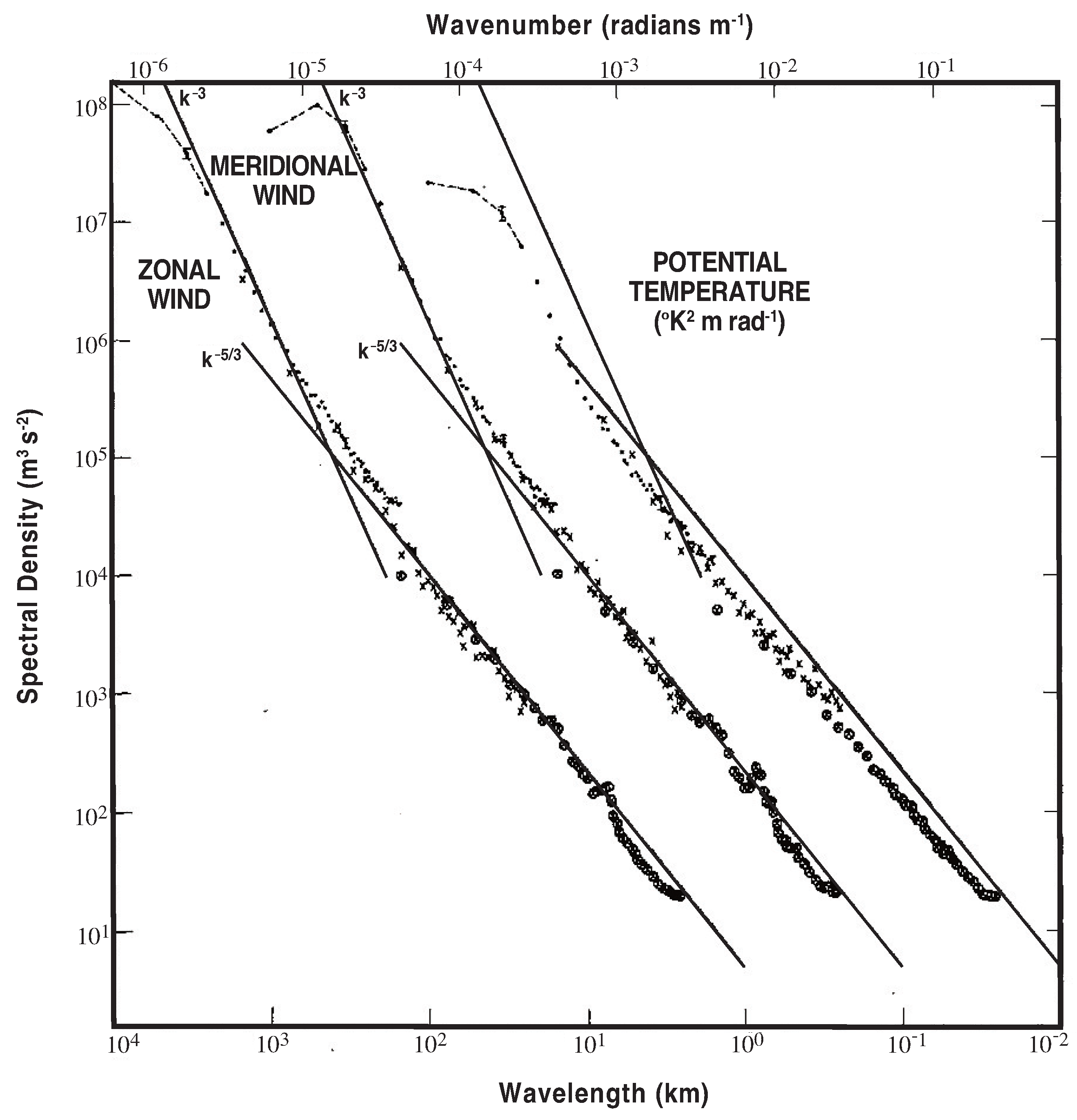
Figure 1 is the celebrated mesoscale horizontal spectra of Nastrom and Gage collected from aircraft flights [8] of the zonal (east–west) wind, the meridional (north–south) wind, and the potential temperature. In this plot, the abscissa denotes the magnitude of the horizontal wave number .
Each spectrum has the functional form of , and the power is between and at large scales and is close to at small scales. Historically, this range was first suspected to be the result of a 2D inverse energy cascade, but later was corroborated by analysis of the 3rd order horizontal velocity structure functions; the direction of energy cascade is regular, i.e., large to small scales [19,20]. The boundary wavenumber between the different powers corresponds to , and for small scales below the energy cascade is enhanced by eddy overturning.
When , since is the smallest scale in the buoyancy dominated region, it can be used as a metric to characterize other length scales. If we assume that the horizontal length scale is associated with the turbulent energy cascade process it can be expressed in terms of the characteristic horizontal velocity U and the rate of energy dissipation as [21]. We further assume that the vertical length scale corresponds to the buoyancy scale . Then, by taking the ratio with , and by expressing the results by the horizontal Froude number, , we have the following relations:
which indicates that holds in the buoyancy dominated region [14].
It was shown that randomly scattered horizontal pancake vortices are the characteristic vortical structures in stably stratified turbulence [7]. Based on the above relations, the ratio of horizontal and vertical length scales of the vortices is given as , .
3. Development of 2dim and 3dim Energy and Spectrum
3.1. Craya–Herring Decomposition
The basic idea of the Craya–Herring decomposition is the following [22]. The Fourier transform of the velocity incompressibility condition provides , where is the wavenumber vector, directly shows that the Fourier transform of the velocity vector, spans two independent basis vectors , in the plane perpendicular to as . As the orthonomal basis vectors, the following expressions follow:
Based on these expressions, and can be calculated explicitly as
where is the Fourier transform of the z-component of vorticity. These expressions define the energy densities and respectively as
From the above equations; we see that is related to the horizontal vorticity while is related to the vertical velocity. Notice that the vertical velocity is coupled with the temperature fluctuation in an oscillatory manner, such as waves, we see that is horizontal and vortical and is vertical and wavy [7].
3.2. Numerical Results
We Fourier transform Equations (1)–(3) and integrate them pseudo-spectrally in a 2 periodic box in the dimensions. Here, the results with grid points are presented. As the external force, we add an integrated white-noise to the horizontal velocity components, and in a narrow waveband at the horizontal wave number .
Starting with zero kinetic energy, we first decouple the equation for the temperature fluctuation from the momentum equations for some time from , thus allowing the forcing to build two-dimensional turbulence uniformly in all horizontal layers in the z direction; is imposed in this first stage. After two-dimensional turbulence is developed, the temperature equation is turned on to see how the energy in grows.
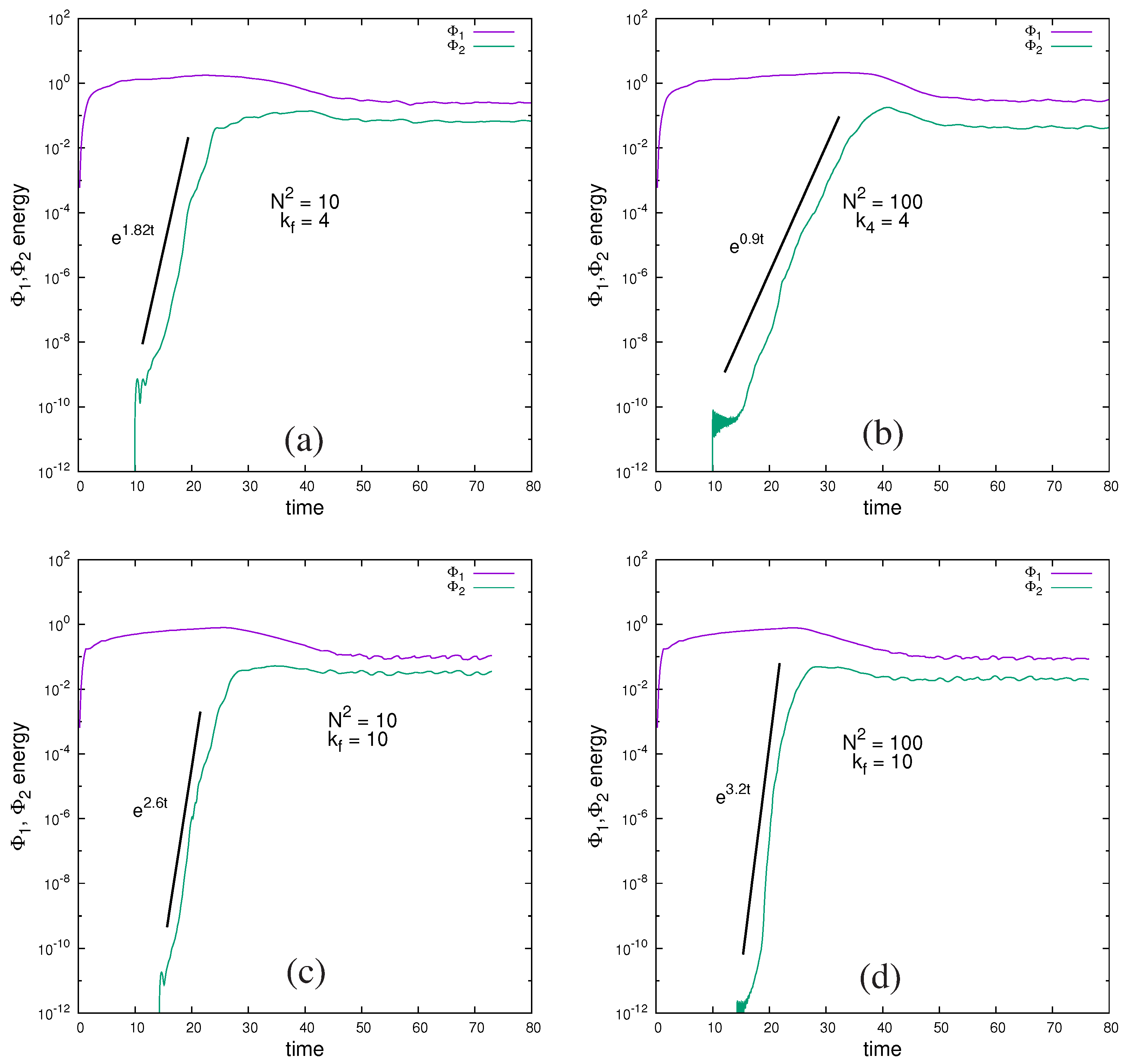
Figure 2 shows the time development of the energy in and , , and , for four different cases, , respectively. For all cases, the development of the features are summarized as follows:
- The energy grows rapidly in a fraction of time after , and continues to increase gradually. Then the equation for the temperature fluctuations is turned on. After a short period of time, the energy begins to grow dramatically at an exponential growth, . The growth rate is larger for than . As the energy in grows comparable to , they begin to interact and the speed and the growth of decreases (and slightly that of as well).
- As the interaction of and grows, and around the time when energy becomes almost 10% of that of , the energy reaches its maximum value, and then begins to decrease. Slightly after that time, reaches its maximum value, followed by a gradual decrease in and .
- At long times, the interaction between and becomes almost stationary and produces small oscillations. The fluctuations in the forcing seems to be the cause of these oscillations. and oscillate almost in phase, which is presumably due to the incompressibility that the Boussinesq approximation assumes.
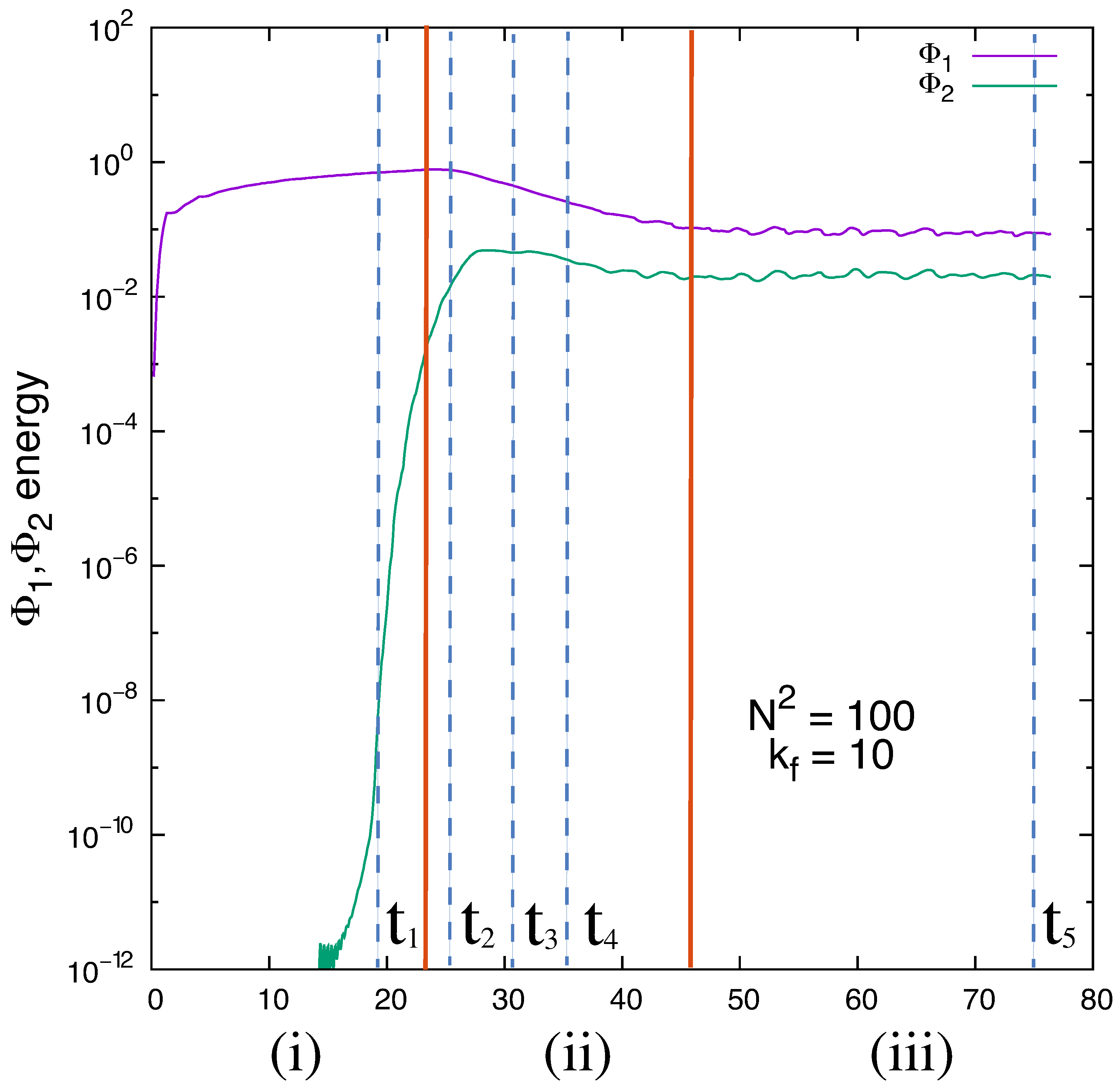
Next, we examine the development of statistical quantities in Figure 2d; the case is an example. Figure 3 spans three time slots marked by orange solid lines, (i) , (ii) , and (iii) , corresponding to the above three characteristic features (1)∼(3). Also in Figure 3, the dashed lines show the times at which the flow features are analyzed in the later analysis.
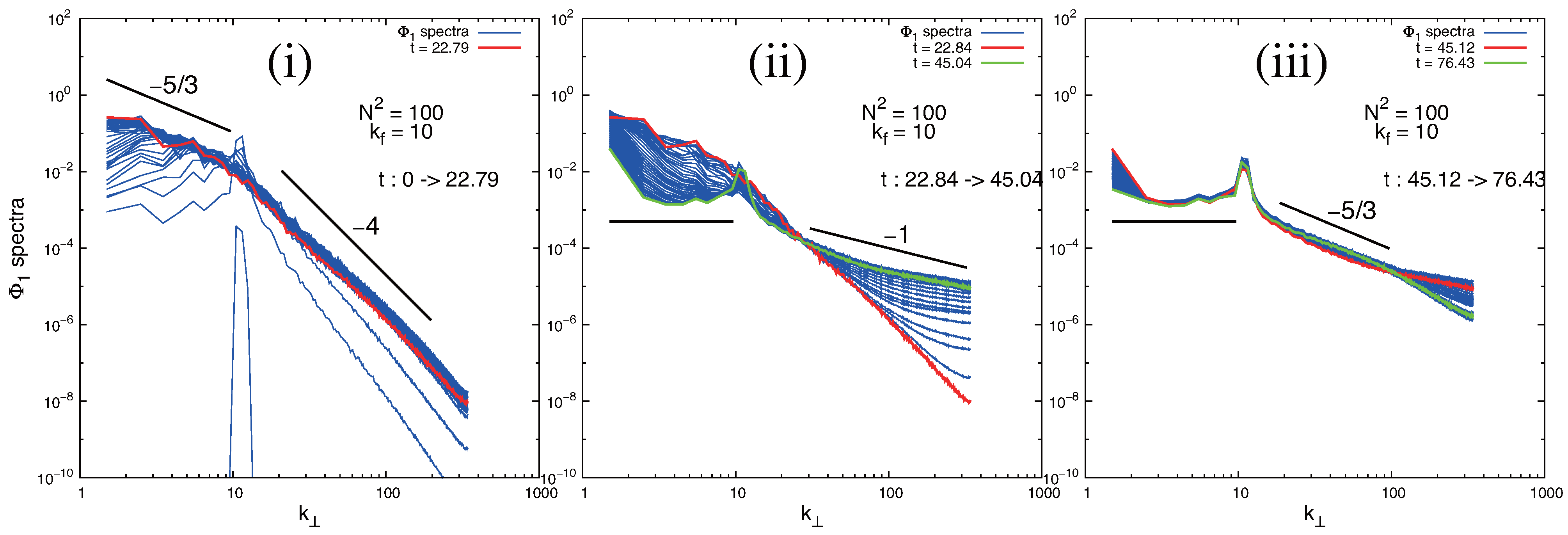
Figure 4i shows the development of the spectra during the (i) time slot in Figure 3. This time interval corresponds to the process of forced two-dimensional turbulence with spectra at scales smaller than the forcing wavenumbers; this corresponds to an inverse cascade of energy. At larger scales, spectra with slopes appear as typical spectra indicating a forward cascade of kinetic energy.
After the equation of the temperature fluctuations is turned on and grows rapidly, the large scale part (small wavenumber part) of the spectra tends to be flat as the small scale part (large wavenumber part) is elevated to be shallow spectra with an exponent approaching (Figure 4ii). It seems obvious that the large scale energy is transferred significantly because of the interaction between and .
When the interaction between and becomes almost stationary, the spectra shows small changes, but tends to show a clear slope at the high regions; at the same time the low spectra become flatter (Figure 4iii).
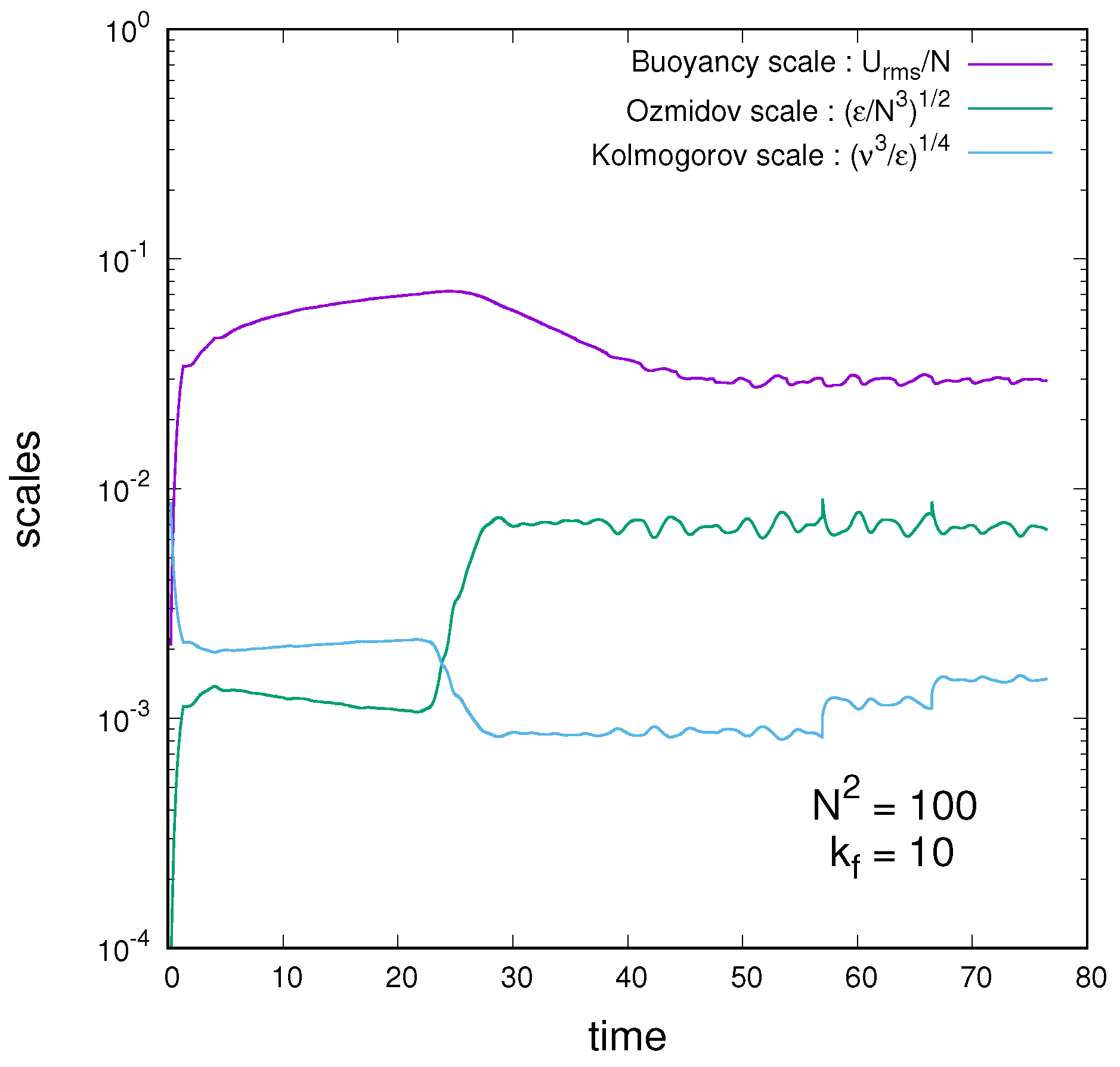
To understand the change in behavior in the spectra, Figure 5 shows the change in the buoyancy, the Ozmidov and the Kolmogorov scales, explained in the previous section. A noteworthy phenomenon is that the Ozmidov, and the Kolmogorov scales cross around at which the buoyancy scale reaches its maximum. In the previous figures, this time corresponds to the time when the 2D state begins to change to 3D by the interaction between waves and vortices. Another interesting point is that the development of the buoyancy scale follows a similar path as in Figure 2 and Figure 3. Throughout the simulation, the buoyancy scale is the largest scale in the flow. The similarity between the buoyancy scale and implies that the horizontal flow continues to dominant, but we have to be a little careful to reach this conclusion—an explanation follows.
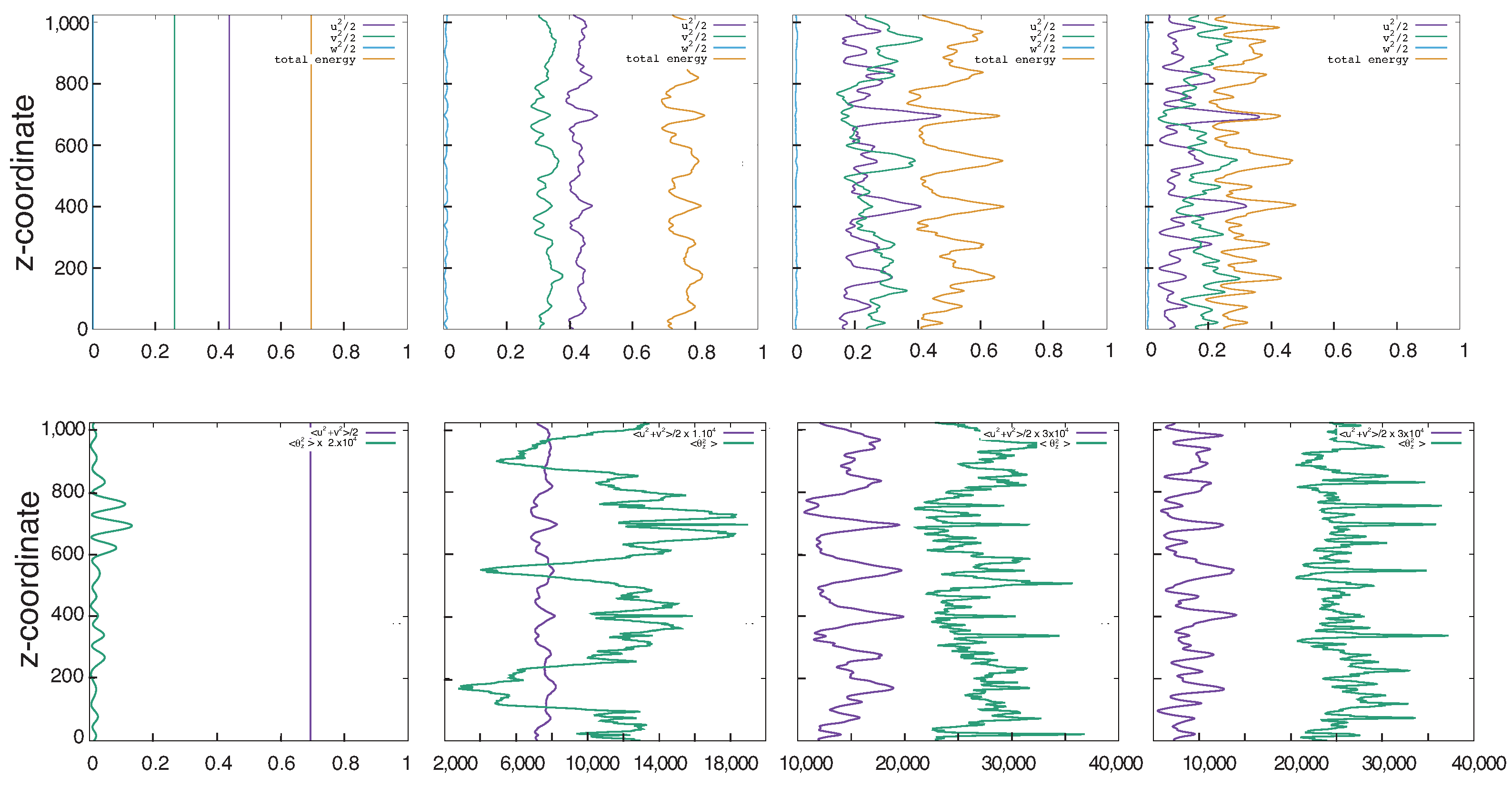
Figure 6 shows the development of the horizontal average of the variances, , , , and the total energy for varying z. Results are shown at in Figure 3 (upper row), and the horizontal average of the horizontal energy, , and monitored also at are the horizontal average of the square of the vertical derivative of temperature fluctuations, (lower row). The following observations can be made:
- (1)
- At , the energy in all directions is uniform in z. The vertical gradient of temperature fluctuations shows small oscillation due to the initial small growth of . The total flow is mainly two-dimensional at this time.
- (2)
- At , fluctuations in the horizontal energy develop, but the vertical energy is still very close to zero. The oscillation of the energy is not uniform, and small deviations in frequency and amplitude are seen. However, the structures in the x and y directions are similar. More striking is the vertical gradient of the temperature fluctuations that shows a few periodic humps with the tops showing stronger oscillations.
- (3)
- At , the energy in the x and y directions, , are in a similar range of magnitude with sharp peaks often at different locations in z. This implies that the velocity field is directionally intermittent, with the kinetic energy sometimes highly concentrated in one direction. Without looking at the coherence of the energy, we cannot readily identify the flow structure, but one possibility is there may at times be uni-directional wind flows.
- (4)
- At , the intermittency in both the energy and the temperature derivative distributions grows. In particular, the peaks of the latter become sharply outstanding from the signals of low but rapid oscillations.
Figure 6.
Upper row: The horizontal average of the energy, (violet), (green), (blue) and the total energy (orange) as a function of z. Lower row: The horizontal average of the horizontal energy, (violet) and the horizontal average of the square of the vertical derivative of temperature fluctuations, (green). All statistics are monitored at in Figure 3.

The above monitoring times, , are all in time slot (ii) in Figure 3 and Figure 4. The characteristic strong intermittent growth during this time slot is attributed to the phenomenon that the 2D energy in the large scales is destroyed with the energy transferred into small scales producing spectra with a nearly slope, much shallower than the Kolmogorov’s spectrum.
The dramatic growth in intermittency in time interval (ii) in Figure 3 and Figure 4 is moderated in time interval (iii). In latter time range, the change in the large scale spectrum and the subsequent energy outflow towards small scales weakens (Figure 4iii), and the small scale spectrum has fallen to the Kolmogorov spectrum. The end part of the spectra at the smallest scales has become steeper than the power, showing a hint of dissipation spectrum. This observation has support if we look at the growth of the Kolmogorov scale at late time in Figure 5. It is interesting that the Kolmogorov scale increases in a stepped manner at and .
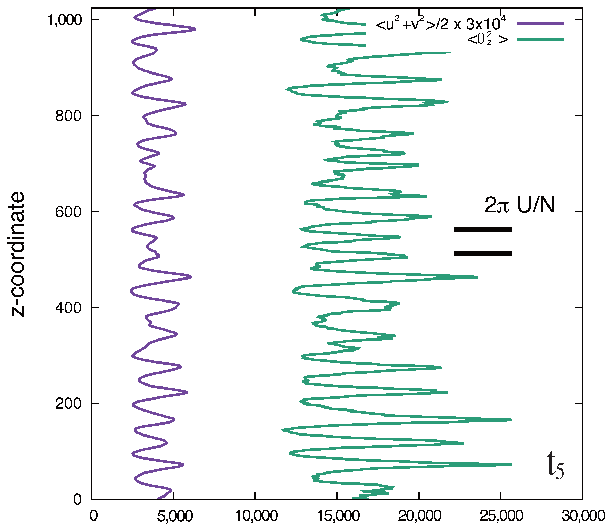
The horizontal average of the horizontal energy, , and the horizontal average of the square of the vertical derivative of temperature fluctuations, , at the time in Figure 3 are shown in Figure 7. After a long time, the oscillatory interaction of and is presumably near equilibrium. The intervals of the peaks are almost equally periodic, which means that the high intermittency of the temperature gradient is softened. The characteristic frequency of the peaks can be compared with the value of in Figure 7. However, the frequency should be related with that of the forcing, and the true reason for the interval is still an open question.
Figure 7.
The horizontal average of the horizontal energy, , and the horizontal average of the square of the vertical derivative of temperature fluctuations, , at about the final time in Figure 3. The characteristic frequency of the peaks is compared with the value of .
Figure 7.
The horizontal average of the horizontal energy, , and the horizontal average of the square of the vertical derivative of temperature fluctuations, , at about the final time in Figure 3. The characteristic frequency of the peaks is compared with the value of .

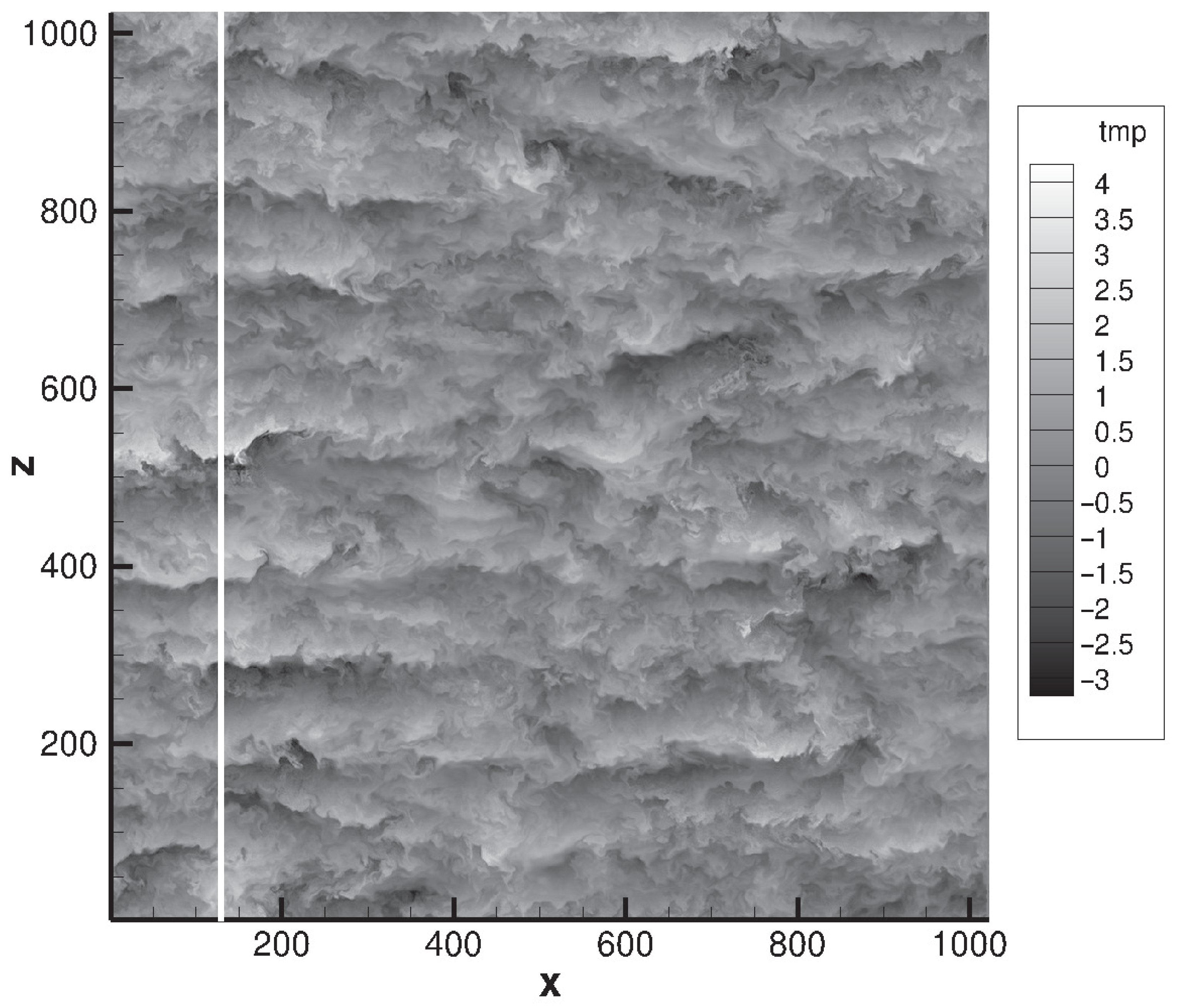
Now we look at the contour plot of the temperature fluctuations in an plane at (grid number 512) for at (Figure 8). (To see the structures clearly, a grey scale is used. The grid number is depicted in the figure as the x and z coordinates).
Many horizontally extended layers are observed which have sharp interfaces between black and white regions. The existence of such interfaces implies that the temperature fluctuations jump at the interfaces. To observe such jumps in temperature fluctuations, its value at is monitored along the white line in Figure 8.
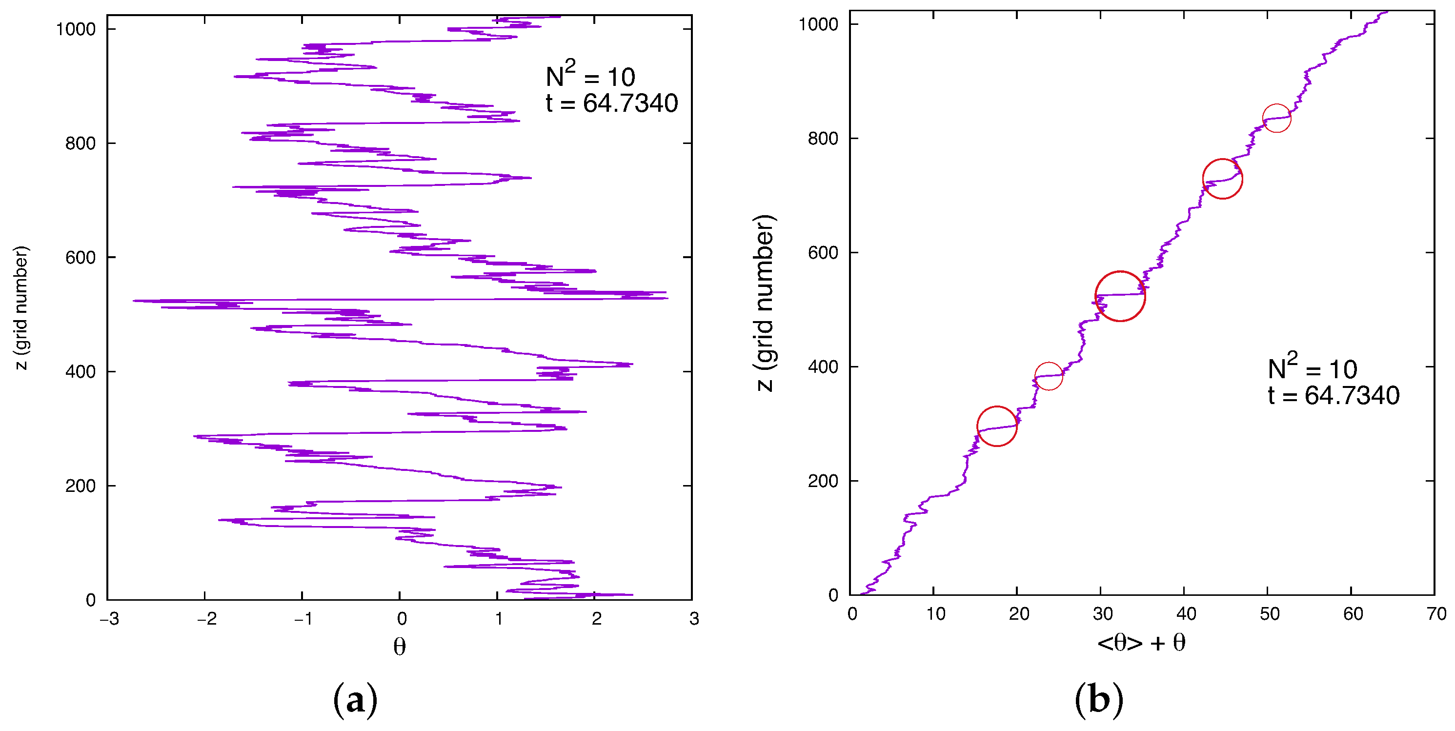
Figure 9a shows the graph of the temperature fluctuation as a function of z (in terms of grid number) along . Horizontally flat and straight lines are observed periodically which are bridged by finely oscillatory stairs.
In Figure 9b, the saw-tooth pattern of Figure 9a is superposed with the mean temperature, , corresponding to . The overall saw-tooth structures in Figure 9a produce cliff–ramp structures in the total temperature field. (Major cliffs are marked with red circles). Temperature jumps at the height of the cliffs. In other words, the cliffs form the interface between cold and warm fluid masses. The most characteristic feature of the cliff–ramp structures is that ramps are mostly leftward (i.e., cooling as it goes up) with jitters. Similar temperature front structures are observed in simulations of homogeneous shear flows [23,24] as well as in large-eddy simulations of the stably stratified atmospheric boundary layer [25].
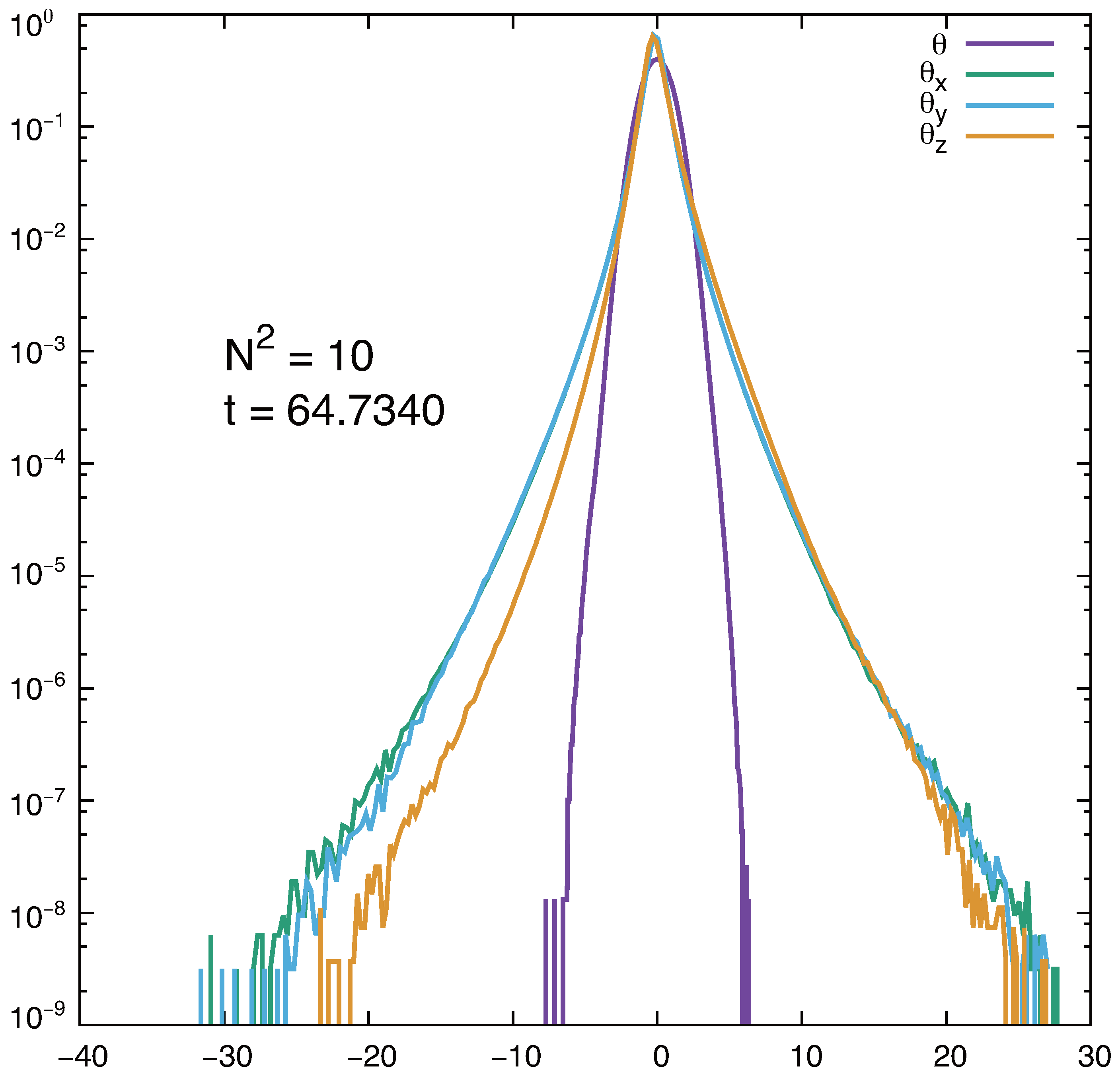
To compensate for the cooling ramps, cliffs should be warming as it goes up. Therefore, there is an asymmetry in the slope of the temperature distribution. Such asymmetry is clearly seen statistically if we look at the PDFs of temperature fluctuation and its derivatives in the whole domain (Figure 10).
In Figure 10, the PDF of temperature fluctuation is close to Gaussian, while those of its derivatives show exponential tails. Among the three derivatives, the derivatives in x- and y- are symmetric, while the z- derivative is skewed with the positive values being higher probability. This statistics supports the phenomenon that the cliffs are associated more with warming.
4. Discussion
Apparently it appears odd that the integration of the Navier–Stokes equations with periodic boundary conditions produces non-symmetric statistics of the derivative of the temperature fluctuations. However, we can check that the integration of in z is zero which is compatible with the periodic boundary condition. Even under this circumstance, we suspect that the intermittent velocity components (Figure 6) acting as a strong horizontal “wind” may produce a non-symmetric gradient of temperature fluctuations. Nevertheless, clarification of the true mechanism is still an open question.
The present research on the development of structures and spectra in stably stratified turbulence is largely related to the broad study of mixing and transport in turbulence. This old and important subject has been investigated by many researchers. The reader is referred to some of the basic reviews and the references therein for the historic and recent developments [18,26,27,28,29].
Author Contributions
Conceptualization and methodology including software, Y.K. and P.P.S.; validation, P.P.S.; writing—original draft preparation, Y.K.; writing—review and editing, P.P.S.; visualization, Y.K.; supervision, P.P.S.; funding acquisition, Y.K. All authors have read and agreed to the published version of the manuscript.
Funding
Y.K. is funded by JSPS (Japan Society for the Promotion of Science) KAKENHI (Grants-in-Aid for Scientific Research), grant number 19H00641 to conduct this reseach.
Institutional Review Board Statement
Not applicable.
Informed Consent Statement
Not applicable.
Data Availability Statement
The data presented in this study are available on request from the corresponding author due to privacy.
Acknowledgments
The final part of this paper is based on the talk presented in the VIIIth International Symposium on Stratified Flows, (29 August–1 September 2016, San Diego, CA, USA) [30]. Jack was one of the authors of this presentation. We were preparing for publicizing the result, but we could not finish it. This paper is dedicated to the memory of Jack Herring.
Conflicts of Interest
The authors declare no conflict of interest.
References
- Kimura, Y.; Herring, J.R. Diffusion in stable stratified turbulence. J. Fluid Mech. 1996, 328, 253–269. [Google Scholar] [CrossRef]
- Csanady, G.T. Turbulent diffusion in a stratified fluid. J. Atmos. Sci. 1964, 21, 439–447. [Google Scholar] [CrossRef]
- Cox, C.Y.; Nagata, Y.; Osborn, T. Oceanic fine structure and internal waves. Papers in dedication to Prof. Michitaka Uda. Bull. Jpn. Soc. Oceanogr. 1969, 1, 67–71. [Google Scholar]
- Lilly, D.K.; Walko, D.E.; Adelfang, S.I. Stratospheric Mixing estimated from high-altitude turbulence measurements. J. Appl Met. 1974, 13, 488–493. [Google Scholar] [CrossRef]
- Weinstock, J. Vertical turbulent diffusion in a stably stratified fluid. J. Atmos. Sci. 1978, 35, 1022–1027. [Google Scholar] [CrossRef]
- Pearson, H.J.; Puttock, J.S.; Hunt, J.C.R. A Statistical model of fluid<lement motions and vertical diffusion in a homogeneous stratified turbulent flow. J. Fluid Mech. 1983, 129, 219–249. [Google Scholar]
- Kimura, Y.; Herring, J.R. Energy spectra of stably stratified turbulence. J. Fluid Mech. 2012, 698, 19–50. [Google Scholar] [CrossRef]
- Nastrom, G.D.; Gage, K.S. A climatology of atmospheric wavenumber spectra of wind and temperature observed by commercial aircraft. J. Atmos. Sci. 1985, 42, 950–960. [Google Scholar] [CrossRef]
- Riley, J.J.; de Bruyn Kops, S.M. Dynamics of turbulence strongly influenced by buoyancy. Phys. Fluids 2003, 15, 2047–2059. [Google Scholar] [CrossRef]
- Waite, M.L.; Bartello, P. Stratified turbulence dominated by vortical motion. J. Fluid Mech. 2004, 517, 281–308. [Google Scholar] [CrossRef]
- Bartello, P.; Tobias, S.M. Sensitivity of stratified turbulence to the buoyancy Reynolds number. J. Fluid Mech. 2013, 725, 1–22. [Google Scholar] [CrossRef]
- Portwood, G.D.; de Bruyn Kops, S.M.; Taylor, J.R.; Salehipour, H.; Caulfield, C.P. Robust identification of dynamically distinct regions in stratified turbulence. J. Fluid Mech. 2016, 807, R2. [Google Scholar] [CrossRef]
- Lucas, D.; Caulfield, C.P.; Kerswell, R.R. Layer formation in horizontally forced stratified turbulence: Connecting exact coherent structures to linear instabilities. J. Fluid Mech. 2017, 832, 409–437. [Google Scholar] [CrossRef]
- Brethouwer, G.; Billant, P.; Lindborg, E.; Chomaz, J.-M. Scaling analysis and simulation of strongly stratified turbulent flows. J. Fluid Mech. 2007, 585, 343–368. [Google Scholar] [CrossRef]
- Spalart, P.R.; Moser, R.D.; Rogers, M.M. Spectral methods for the Navier–Stokes equations with one infinite and two periodic directions. J. Comput. Phys 1991, 96, 297–324. [Google Scholar] [CrossRef]
- Doughtery, J.P. The anisotropy of turbulence at the meteor level. J. Atmos. Sci. 1961, 21, 210–213. [Google Scholar]
- Ozmidov, R.V. On the turbulent exchange in a stably stratified ocean. Izv. Atmos. Ocean. Phys. Ser. 1965, 21, 210–213. [Google Scholar]
- Caulfield, C.P. Layering, Instabilities, and Mixing in Turbulent Stratified Flows. Annu. Rev. Fluid Mech. 2021, 53, 113–145. [Google Scholar] [CrossRef]
- Cho, J.Y.N.; Lindborg, E. Horizontal velocity structure functions in the upper troposphere and lower stratosphere 1. Observations. J. Geophys. Res. 2001, 106, 10223–10232. [Google Scholar] [CrossRef]
- Lindborg, E.; Cho, J.Y.N. Horizontal velocity structure functions in the upper troposphere and lower stratosphere 2. Theoretical considerations. J. Geophys. Res. 2001, 106, 10233–10241. [Google Scholar] [CrossRef]
- Maffioli, A.; Davidson, P.A. Dynamics of stratified turbulence decaying from a high buoyancy Reynolds number. J. Fluid Mech. 2016, 786, 210–233. [Google Scholar] [CrossRef]
- Sagaut, P.; Cambon, C. Homogeneous Turbulence Dynamics; Cambridge University Press: Cambridge, UK, 2008. [Google Scholar]
- Gerz, T.; Howell, J.; Mahrt, L. Vortex structures and microfronts. Phys. Fluids 1994, 6, 1242–1251. [Google Scholar] [CrossRef]
- Chung, D.; Matheou, G. Direct numerical simulation of stationary homogenous stratified sheared turbulence. J. Fluid Mech. 2012, 696, 434–467. [Google Scholar] [CrossRef]
- Sullivan, P.P.; Weil, J.C.; Patton, E.G.; Jonker, H.J.J.; Mironov, D.V. Turbulent winds and temperature fronts in large eddy simulations of the stable atmospheric boundary layer. J. Atmos. Sci. 2016, 73, 1815–1840. [Google Scholar] [CrossRef]
- Fernando, H.J.S. Turbulent mixing in stratified fluids. Annu. Rev. Fluid Mech. 1991, 23, 455–493. [Google Scholar] [CrossRef]
- Peltier, W.R.; Caulfield, C.P. Mixing efficiency in stratified shear flows. Annu. Rev. Fluid Mech. 2003, 35, 135–167. [Google Scholar] [CrossRef]
- Ivey, G.N.; Winters, K.B.; Koseff, J.R. Density stratification, turbulence, but how much mixing. Annu. Rev. Fluid Mech. 2008, 40, 169–184. [Google Scholar] [CrossRef]
- Gregg, M.C.; D’Asaro, E.A.; Riley, J.J.; Kunze, E. Mixing efficiency in the ocean. Annu. Rev. Mar. Sci. 2018, 10, 443–473. [Google Scholar] [CrossRef]
- Kimura, Y.; Sullivan, P.P.; Herring, J.R. Temperature front formation in stably stratified turbulence. In Proceedings of the VIIIth International Symposium on Stratified Flows, San Diego, CA, USA, 29 August–1 September 2016. [Google Scholar]
Figure 1.
Nastrom-Gage spectrum ([8]) From the left, the zonal (east-west) wind, the meridional (north-south) wind, and the potential temperature. Each has the functional form of , and the power is between and at large scales and near at small scales.
Figure 1.
Nastrom-Gage spectrum ([8]) From the left, the zonal (east-west) wind, the meridional (north-south) wind, and the potential temperature. Each has the functional form of , and the power is between and at large scales and near at small scales.

Figure 2.
Development of and energy as a function of time: (a) , , (b) , , (c) , and (d) .

Figure 3.
Division of the time intervals along Figure 2d: (i) , (ii) , and (iii) . (the boundary of these intervals are given as red lines) are the times at which statistics are shown in Figures 6 and 7.
Figure 3.
Division of the time intervals along Figure 2d: (i) , (ii) , and (iii) . (the boundary of these intervals are given as red lines) are the times at which statistics are shown in Figures 6 and 7.

Figure 4.
Development of spectra in the time interval (i–iii) in Figure 3. Red and green colors correspond to the initial and the last time in each interval.
Figure 4.
Development of spectra in the time interval (i–iii) in Figure 3. Red and green colors correspond to the initial and the last time in each interval.

Figure 5.
Growth of the tree scales, buoyancy, Ozmidov, and Kolmogorov scales for , .

Figure 8.
Temperature fluctuations in an plane at (grid number 512) for at .

Figure 9.
(a) Temperature fluctuation as a function of z (in grid number) along in Figure 8 (white line). (b) The saw-tooth graph of (a) is superposed with the mean temperature, , corresponding to . Cliff–ramp structures are seen, and major cliffs are marked with red circles.
Figure 9.
(a) Temperature fluctuation as a function of z (in grid number) along in Figure 8 (white line). (b) The saw-tooth graph of (a) is superposed with the mean temperature, , corresponding to . Cliff–ramp structures are seen, and major cliffs are marked with red circles.

Figure 10.
PDFs of temperature fluctuation and its derivatives in the whole domain. The PDF of temperature fluctuation is close to Gaussian, while those of its derivatives show exponential tails. The derivatives in x- and y- are symmetric, while the z- derivative is skewed.
Figure 10.
PDFs of temperature fluctuation and its derivatives in the whole domain. The PDF of temperature fluctuation is close to Gaussian, while those of its derivatives show exponential tails. The derivatives in x- and y- are symmetric, while the z- derivative is skewed.

Disclaimer/Publisher’s Note: The statements, opinions and data contained in all publications are solely those of the individual author(s) and contributor(s) and not of MDPI and/or the editor(s). MDPI and/or the editor(s) disclaim responsibility for any injury to people or property resulting from any ideas, methods, instructions or products referred to in the content. |
© 2024 by the authors. Licensee MDPI, Basel, Switzerland. This article is an open access article distributed under the terms and conditions of the Creative Commons Attribution (CC BY) license (https://creativecommons.org/licenses/by/4.0/).
Share and Cite
MDPI and ACS Style
Kimura, Y.; Sullivan, P.P. 2D and 3D Properties of Stably Stratified Turbulence. Atmosphere 2024, 15, 82. https://doi.org/10.3390/atmos15010082
AMA Style
Kimura Y, Sullivan PP. 2D and 3D Properties of Stably Stratified Turbulence. Atmosphere. 2024; 15(1):82. https://doi.org/10.3390/atmos15010082
Chicago/Turabian StyleKimura, Yoshifumi, and Peter P. Sullivan. 2024. "2D and 3D Properties of Stably Stratified Turbulence" Atmosphere 15, no. 1: 82. https://doi.org/10.3390/atmos15010082
Note that from the first issue of 2016, this journal uses article numbers instead of page numbers. See further details here.