Article

Investigating the Complexities of VOC Sources in Mexico City in the Years 2016–2022

by
Mohammad Jahirul Alam
1,2,
Bernhard Rappenglueck
1,2,*,
Armando Retama
3 and
Olivia Rivera-Hernández
4
1
Department of Earth and Atmospheric Sciences, University of Houston, Houston, TX 77204, USA
2
Institute for Climate and Atmospheric Science, University of Houston, Houston, TX 77204, USA
3
Independent Researcher, Mexico City C.P. 06000, Mexico
4
Dirección de Monitoreo de Calidad del Aire, Secretaría del Medio Ambiente, Mexico City C.P. 06000, Mexico
*
Author to whom correspondence should be addressed.
Atmosphere 2024, 15(2), 179; https://doi.org/10.3390/atmos15020179
Submission received: 31 December 2023 / Revised: 26 January 2024 / Accepted: 28 January 2024 / Published: 31 January 2024

Abstract

:
Volatile organic compounds (VOCs) are major ingredients of photochemical smog. It is essential to know the spatial and temporal variation of VOC emissions. In this study, we used the Positive Matrix Factorization (PMF) model for VOC source apportionment in Mexico City. We first analyzed a data set collected during the ozone season from March–May 2016. It includes 33 VOCs, nitrogen oxide (NO), nitrogen dioxide (NO2), the sum of nitrogen oxides (NOx), carbon monoxide (CO), sulfur dioxide (SO2) and particle matter with a diameter < 1 μm (PM1). Another PMF analysis focused only on VOC data obtained in the month of May between the years 2016, 2017, 2018, 2021, and 2022 to gain insights into interannual variations. While the use of fossil fuel through combustion and evaporation continues to be major fraction in Mexico City, additional sources could be identified. Apart from biogenic sources which become more important closer to the end of the ozone season, a second natural emission factor termed “geogenic”, was identified. Overall, anthropogenic sources range between 80–90%. Diurnal plots and bivariate plots show the relative importance of these emission source factors on different temporal and spatial scales, which can be applied in emission control policies for Mexico City.

1. Introduction

Volatile organic compounds (VOCs) are a wide group of atmospheric organic substances with a high vapor pressure at ambient temperatures [1,2]. As VOCs are oxidized in the troposphere by ozone (O3), nitrate (NO3), hydroxyl (OH), and chlorine (Cl) radicals, they produce intermediates, such as hydroperoxy radicals (HO2) and organic peroxy radicals (RO2), that generate nitrogen oxides (NOx) and impact photochemical reactions [3,4,5], leading to the production of tropospheric O3 [6] and secondary organic aerosols (SOA), among other species [7,8,9]. In addition, several VOCs are categorized as harmful air pollutants and cause adverse short-term or long-term health consequences [10,11], including irritating mucous membranes, eyes, and throat, and cancer [1,12,13,14].
Therefore, to effectively mitigate the harmful impact of VOC emissions in highly industrialized and populated urban areas, it is necessary to assess VOC emission sources and understand their source-receptor relationships. Important tools include source apportionment models to identify and distinguish emissions in combination with polar scatter plots, which provide valuable insights into the spatial distribution of emission sources.
The Mexico City Metropolitan Area (MCMA) is located in central Mexico, in an elevated basin with an altitude of 2200–2300 m above sea level (a.s.l) enclosed by mountain ranges on three sides and some openings in the north and southwest [15]. This specific topography impacts the local meteorology and climate [16] and leads to thermal inversions and pollutant stagnation, as demonstrated for a recent ozone event [17].
The ozone season, which occurs during the dry warm period between March and May, provides favorable conditions for photochemical reactivity, leading to O3 formation [18]. According to [19], increasing hydrocarbon (HC) emissions during daytime in Mexico City leads to higher ozone levels, while increasing nitrogen oxide (NOx) emissions results in lower ozone levels. However, recent findings [20] point to a more complex relation depending on the specific location within the MCMA. Due to its significant emissions, resulting from a densely populated area with over 21 million inhabitants spread across 7866.1 km2, 6.3 million residential units, 6 million automobiles, 1900 regulated industrial facilities and 2800 businesses, and a plethora of regulated services such as gas stations, repair shops, catering service, and laundry services, the MCMA poses a severe threat to its residents’ environment and health [21].
Earlier research [22] investigated the sources of non-methane hydrocarbon (NMHC) emissions by applying the Chemical Mass Balance (CMB) for three sites, Xalostoc, La Merced, and Pedregal in the spring (March) and fall season (November–December), in 1996. They found that in March, the largest contribution to the ambient NMHC concentrations came from vehicular exhaust at La Merced (60.4%), followed by Xalostoc (52%), and Pedregal (55.3%). With regard to Liquified Petroleum Gas (LPG) emissions, the highest contribution was observed at Xalostoc (29.4%), followed by La Merced (25.4%) and Pedregal (15.4%). In November, La Merced still had the highest contribution from vehicular exhaust emissions, followed by Pedregal and Xalostoc, with increases of 6.9%, 4.2%, and 1.8%, respectively, when compared to the data from March. LPG emissions experienced an increase at all the three sites in November in comparison to March, with the Pedregal site observing the largest increase of 9.1%, followed by La Merced with a 2.9% increase, and Xalostoc with a 1.8% increase, ref. [23] utilized the CMB receptor model to investigate emissions sources at the same sites in Mexico City, from February to March in 1997. Their findings indicated that vehicle sources, specifically gasoline and diesel, were the primary contributing factor, accounting for 58% of total emissions at all the three measurement sites, with Pedregal having the highest contribution from vehicular exhaust and Xalostoc having the highest contribution from LPG. The percentages of contribution were 58% and 15% at La Merced, 50% and 22% at Xalostoc, and 59% and 21% at Pedregal for vehicular exhaust and LPG, respectively. In summary, these two studies, performed in the late 1990s, found that vehicular exhaust and LPG emissions were highest in certain areas of Mexico City in March, with Pedregal having the highest vehicle source contribution and Xalostoc having the highest LPG contribution, but both sources showed an overall decrease from 1996 to 1997 [22,23].
Earlier research [24] found that the concentration of more than 50 VOCs could have stabilized or decreased in Mexico City during 2002–2003, while ref. [25] identified a decrease observed in alkanes and aromatics, but an increase in alkenes in the MCMA between 2000 and 2007. These studies may explain why efforts to reduce ozone and fine aerosols have had only moderate success in those years [18], as the decrease of less reactive alkanes and aromatics might have been compensated by the increase of higher reactive alkenes. Ref. [18] revisited La Merced, and Pedregal NMHC data for the years between 2003 and 2012 and performed updated source apportionment studies. The study revealed that the primary sources of NMHCs in the city remained vehicle traffic, evaporative emissions from fossil fuels and solvents, and LPG consumption. While reductions in alkanes and aromatics totaling 12% and 50% were identified at both sites, respectively, the mixing ratios of alkenes, except ethylene and trans-2-butene, increased by 10% and 16% at La Merced and Pedregal, respectively, over that decade.
Vega et al. [26] conducted a source apportionment study for the same two sites, Merced and Pedregal, in 2006 and 2012 and identified more factors compared to ref. [18]. Their study suggested a mixture of sources caused by correlations among the variables that were not separated by the Positive Matrix Factorization (PMF). In addition, ref. [26] included carbonyls in the PMF input data, which have modified the contribution of the factors. Their analysis revealed that LPG and food cooking (Food C) were primary sources at Merced, decreasing by 1.5% and 3.7%, respectively, while LPG/Food C and light duty vehicle (LDV) exhaust were the main sources at Pedregal, with LPG/Food C increasing by 7.9% and LDV decreasing by 3.3% from 2006 to 2012, and that LPG leakage was found to be about 4–8% less in their PMF analysis compared to around 11% according to the 2006 Emission Inventory [27,28]. Over this 6-year period, all of the aromatics as well as the acetylene decreased, while some alkanes and alkenes showed both decreasing and increasing trends at the Merced and Pedregal sites.
For the year 2006, ref. [26] studied VOCs at Tepeji and Jasso. While those two sites are located outside the MCMA, their study provided insights into additional source signatures as they included carbonyls. For instance, they found that apart from heavy-duty vehicles, domestic heating/cooking were also among the top emission sources at the Jasso site, whereas plastic manufacturing and heating/cooking were predominant VOC sources at the Tepeji site. The further expansion of available pollutants led to a better resolution of source contributions and, thus, to a deeper insight of the variety of emission sources impacting a receptor site.
Recent studies [29] have recently applied the PMF model to identify major emission sources contributing to O3 formation during a severe O3 episode in the MCMA. Their findings indicate that traffic exhaust is the primary contributor to air pollution (48.8%), followed by fuel combustion and evaporation (30.2%), while secondary aerosol precursors and geogenic sources contribute 11.9% and 9.1%, respectively. While geogenic sources of aerosols have been documented in the region [30], the PMF model indicates that VOCs may also be present in geogenic sources.
The CMB and PMF models are two distinct techniques utilized for determining the extent to which various sources of emissions contribute to air pollution at specific locations [31]. The CMB model uses both chemical species concentrations with uncertainties and source fingerprints, while the PMF model only relies on chemical species concentrations with uncertainties since the model generates the factor/source profiles as outputs [32]. The CMB model is susceptible to the choice of sources used and the similarity of their tracers [33]. On the other hand, the PMF model is capable of identifying specific factors/sources and handling missing data and outliers, making it a more versatile tool for analyzing complex datasets with high variability [32,34].
The goals of this research are (1) to investigate the sources of VOCs emissions using a wide range of datasets during the ozone season, between March and May 2016, (2) to utilize a commixture of primarily emitted gas–phase compounds, including VOCs, CO, SO2, NO, NOx, and particulate matter (PM1), to explore a larger breakdown of potential emission factors compared to previous research (Mugica et al., 2003 [23]; Vega et al., 2022 [26]), including further studies on the potential geogenic source of VOCs proposed by [29]. PMF is more appropriate than CMB for source apportionment in cases of insufficient knowledge of local source emission characteristics, as the latter is sensitive to source profiles [31], while PMF factors can represent robust result for mixtures of primary and secondary compounds with contributions from multiple sources, as demonstrated by [31]. Therefore, this study (3) expands on earlier studies emission source and ratio analysis in the MCMA area (e.g., [26]), using diurnal plots and bivariate plots of source factors extracted from PMF, to identify the relative importance of these emission source factors on different temporal and spatial scales, which can be applied in emission control policies for Mexico City.

2. Materials and Methods

2.1. Measurements Setup

The Environmental Analysis Laboratory (EALab; 19.48° N, 99.15° W; 2255 m a.s.l.) of the Atmospheric Monitoring System (SIMAT, by its Spanish acronym) carried out continuous monitoring of VOCs, criteria pollutants such as nitrogen monoxide (NO), nitrogen dioxide (NO2), carbon monoxide (CO), nitrogen oxides (NOx), sulphur dioxide (SO2), and particulate matter with diameter < 1 μm (PM1), along with surface meteorological parameters such as temperature, humidity, relative humidity, wind speed, and wind direction, from 1 March to 31 May 2016. Detailed description of the measurements are described in [29]. Briefly, VOCs in the range of C2–C12 were analyzed using a PerkinElmer gas chromatograph (GC) Clarus ATX 580 (Waltham, MA, USA) and a TurboMatrix Thermal Desorber (model 650 ATD) equipped with two chromatographic columns. Measurement precision was <10% for different components, and limits of detection < 0.1 ppbv. Data of NO, NO2, NOx, CO, and SO2 were retrieved as hourly values from the local air quality monitoring network using commercial (precision of ±10%). PM1 hourly mass concentration was determined using Tapered Element Oscillating Microbalance monitors (TEOM Model 1400AB, Rupprecht & Patashnik Co., Inc., Albany, NY, USA) coupled with a Filter Dynamics Measurement System (FDMS) and equipped with standard PM10 inlet followed by a 1 µm cut-size cyclone (SCC 2.229, BGI, Butler, NJ, USA), set to a flow rate of 16.67 L min−1.

2.2. Emission Source Identification by PMF

Here, we apply the United States Environment Protection Agency’s Positive Matrix Factorization model (EPA PMF 5.0; [35]). The PMF model, developed by [36,37,38], is a receptor model that aims to solve the chemical mass balance between the concentration and the factor profiles of each species. The optimal number of factors in the Positive Matrix Factorization (PMF) analysis was determined using three error estimation methods: bootstrapping, displacement mapping, and bootstrap-displacement. Uncertainties in the factors were estimated using a method described by [38].
We consider the signal, dij, as the ratio between the difference of the concentration (xi) and the uncertainty (ui), and ui. In case xijuij, dij is considered zero (Equation (1)). However, if xij > uij, Equation (2) was utilized. Finally, the signal-to-noise (S/N) ratio was computed by averaging the dij values for each sample, using Equation (3).
d i j = 0
d i j = ( x i j u i j u i j )
( S N ) j = 1 n i = 1 n d i j
In accordance with the aforementioned criteria, a total of 38 air pollutant species, including 33 VOCs, NO, NO2, CO, SO2, and PM1 were selected for the purpose of conducting a PMF analysis.
The selected species were first subjected to classification into three categories, namely “strong”, “weak”, and “bad”, based on their respective signal-to-noise ratios (S/N) and observed/predicted values (R2), as prescribed by [35]. The final number of factors were confirmed by several statistical metrics, including a percentage change in dQ, swaps by BS-DISP, and Qrobust/Qexpected, as determined by principal component analysis.
Qexpected is a calculation used in the positive matrix factorization (PMF) to determine the expected value of the Q metric, which assesses the fit of the model to the data. The Qexpected value is calculated using the following formula:
Qexpected = (N × P) − [(F × N) + (F × P)]
where N is the total number of samples, P is the number of strong species, and F is the number of factors being considered. The Qexpected value represents the minimum value that the Q metric should achieve in a satisfactory PMF model fit. If the calculated Q value is less than the Qexpected value, then the model is considered to be satisfactory. For example, in the current study, for 9 factors F, 38 samples N, and 34 strong species P, Qexp equals 644 (Qexp = (38 × 34) − (4 × 38) + (4 × 34)). Here, moving from 7 to 8 factors leads to a decrease in Qrob/Qexp from 104.3 to 99.54, and while moving from 9 to 10 factors a smaller decrease in Qrob/Qexp from 99.54 to 83.72 is observed, suggesting a nine-factor solution may be the appropriate number of factors (see Table S1). This change is a necessary, albeit not a sufficient criterion. Finally, analyzing the error estimation (DISP, BS, and BS-DISP), the appropriate number of factors can be selected. In the analysis that involved nine factors, there were no changes in the %dQ and no swaps were made in the DISP analysis. All of the factors were consistently mapped with 100% bootstrap factors with regard to base factors in 20 runs, as shown in Table S2. Additionally, there were >80% of the cases found in the bootstrap-displacement (BS-DISP) analysis of the DISP analysis, when nine factors were resolved. This is well above the 50% threshold considered acceptable according to [39].

2.3. PMF Method and Error Estimation

As mentioned before, the PMF model aims to solve the chemical mass balance between the concentration and the factor profiles of each species. This is achieved by minimizing the Q value, which is determined based on the estimated uncertainties (uij) and by considering the mass contribution (gik) of the k-th source to the i-th sample and the residual (eij) of the j-th species to the i-th sample.
x i j = k = 1 p g i k f k j + e i j
Q = i = 1 n j = 1 m [ x i j k = 1 p g i k f k j u i j ] 2
Paatero’s Positive Matrix Factorization (PMF) offers two versions of the Q value: Qtrue and Qrob. Qrob only considers well-fitted data points, with eij/uij < 4, while Qtrue considers all data points. PMF uses two sets of data files for the analysis: concentration and uncertainty. Prior to the PMF run, species with more than 60% of missing values are removed, and concentration values below the compound-specific method detection limit (MDLj) are replaced by 0.5 × MDLj. Missing values are substituted by the median concentration, and outlier values are defined as solitary values xj > X j ¯ - + 3σj or xj < X j ¯ - − 3σj.
For the uncertainty calculation, Equation (7) was used, in the case of the concentration of given species xj > MDLj:
u j = ( [ z j × x j ) ] 2 + ( 0.5 × M D L j ) 2
where zj is the measurement error fraction of the j-th species expressed as percentage. In case xjMDLj, then the uncertainty was calculated based on Equation (4):
u j = 5 6 × M D L j
Uncertainty values for VOCs were within the range of 5% to 30%, as assigned in the studies conducted by [40,41]. In addition, 8% values were assigned for NO, NO2, CO and SO2, in alignment with earlier analyses [39].

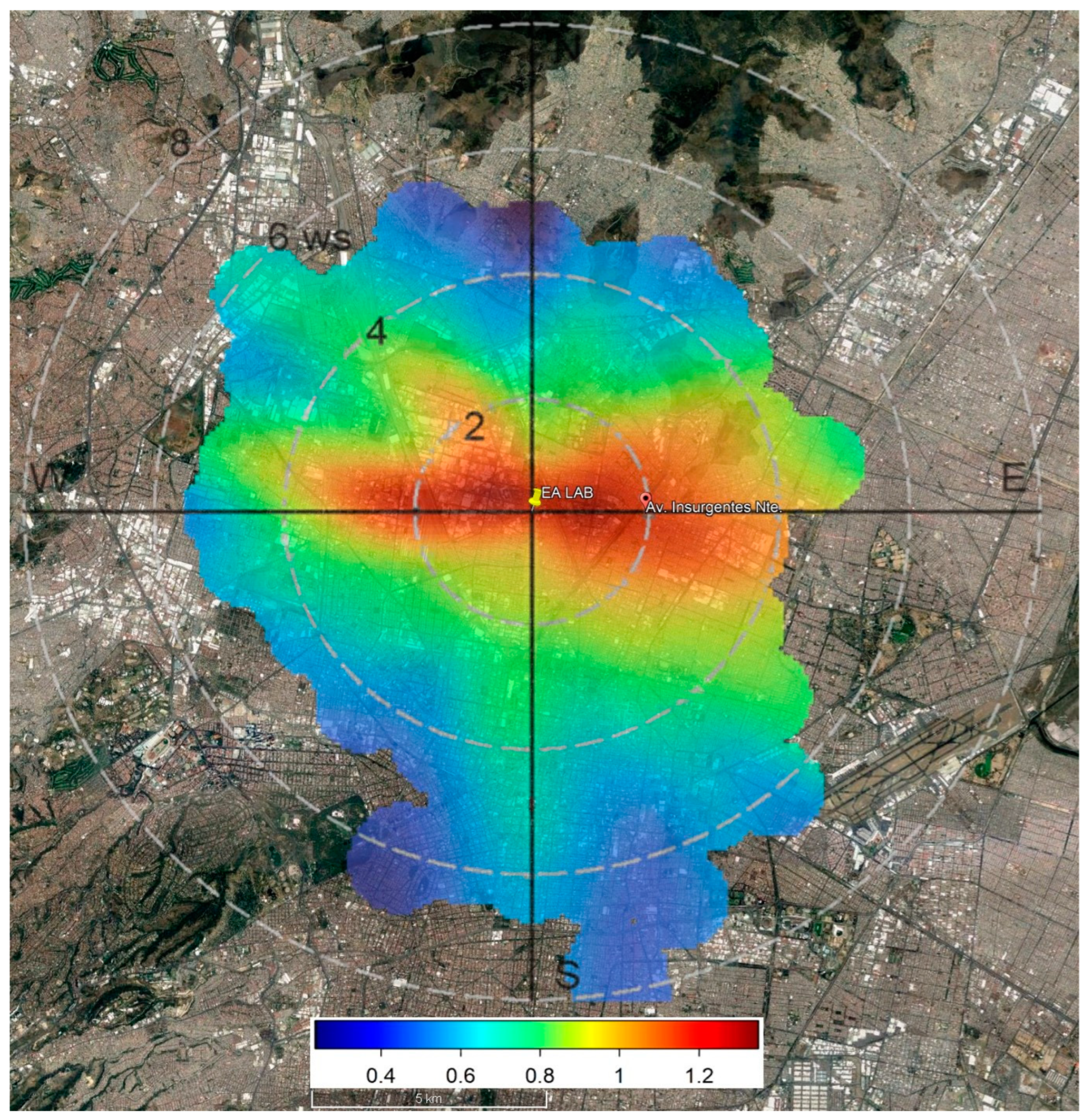
2.4. Bivariate Polar Plots

Our research employs the approach by [42] of generating bivariate polar plots, to identify potential source locations of PMF analysis results, using wind speed and direction data. The openair package in R was employed to generate bivariate polar plots [43], and for interpolation, the package utilized the Generalized Additive Model (GAM) interpolation method, as proposed by [44].
The bivariate polar plots were generated using a Non-Parametric Wind Regression (nwr) approach that relies on Kernel smoothers, as described by [45].

3. Results and Discussion

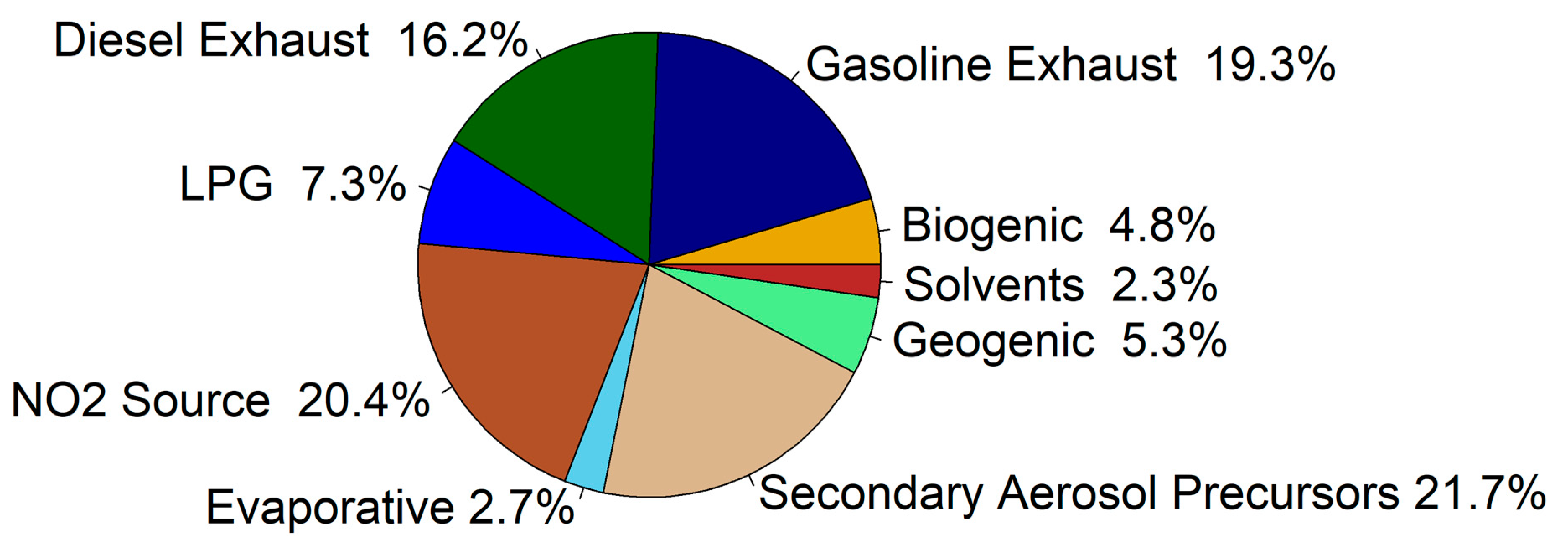
3.1. Source Apportionment

Table S3 shows the statistical results for all trace gases measured during the entire time frame from March to May 2016. The most abundant VOCs were alkanes, with the highest median values for propane (33.27 ppb), n-butane (5.48 ppb), isopentane (3.94 ppb), and ethane (3.86 ppb). Among alkenes, ethylene (4.20 ppb) and propylene (1.45 ppb), and among aromatics, toluene (3.91 ppb), m-&p-xylene (1.63 ppb), and o-xylene (0.65 ppb) showed the highest median mixing ratios. The median mixing ratios of CO, NO, NO2 and SO2 are 500 ppb, 5.4 ppb. 35.0 ppb and 22.3 ppb, respectively.
The PMF analysis yielded nine emission factors (Figure 1). The most significant contributor to atmospheric composition is the factor secondary aerosol precursors, accounting for 21.7% of the total mass, followed by the source factors NO2 (20.4%), gasoline exhaust (19.3%), diesel exhaust (16.2%), with liquefied petroleum gas (LPG) (7.3%), geogenic (5.3%), biogenic (4.8%), evaporative emission (2.7%), and solvents (2.3%) each contributing less than 10% (Figure 2). Overall, anthropogenic sources contribute almost 90%.

3.2. Biogenic Factor

The biogenic factor primarily comprises isoprene, a chemical tracer of biogenic emissions that is predominantly emitted by deciduous trees and shrubs and is known to increase with higher temperatures and solar radiation [46,47,48]. Isoprene showed a high loading of 67.8% of substance mass apportioned to this biogenic factor. Despite being primarily associated with biogenic emissions from trees and shrubs, isoprene can also be emitted into the atmosphere from anthropogenic sources such as vehicle exhaust and human exhalation [49,50,51,52,53,54]. Previous field campaigns did not find a significant biogenic contribution to the VOC burden within the MCMA (Molina et al., 2007, 2010 [55,56]), and some studies [57,58] concluded that observed isoprene was associated with traffic emissions rather than vegetation, which may have been a result of limited study duration [18]. For the first time, ref. [18] found elevated isoprene in Mexico City associated with both traffic and biogenic emissions. They found that the biogenic peak of isoprene became more prominent from March to May, with peak isoprene values occurring between 13:00–15:00 local time (LT), in agreement with the prediction by [59] of the highest isoprene emissions due to the highest solar radiation at the end of the dry-warm season in the Valley of Mexico. Increasing ambient temperature from March to May would be another parameter regulating isoprene emissions [60].
In our study, we found an alignment of the temporal variation of isoprene mixing ratios with CO, a typical tracer for vehicle related emission, in the morning rush hour between 6:00–9:00, which indicates a potential source of traffic-related isoprene emissions (Figure 3), which agrees with earlier findings by [18]. Furthermore, the moderate correlation (R2 = 0.54) between the gasoline combustion tracer acetylene and isoprene during the night and the poor correlation (R2 = 0.08) during the day suggest that isoprene emissions at night may originate from gasoline combustion, according to our study. Figure 3 also shows that in March, isoprene values were highest during the early morning rush hour, while the isoprene peak in the afternoon increased from March to May with increasing temperature and global radiation.
The findings from the biogenic polar plot (Figure 4) reveal that the isoprene factor plays a significant role (with levels ranging from 1 to 1.5 μg/m3) when the wind direction was either from the NW or SE directions. Notably, the NW direction was found to be linked to the Sierra de Guadalupe, which is situated approximately 15 km northwest of the study area. Also, the gardens of the National Polytechnic Institute aligned in this direction could be a source area. Additionally, forests in the mountain areas surrounding the MCMA, especially under SE winds, could impact the receptor site.

3.3. Gasoline Exhaust

Factor 2 is predominated by ethylene (59.7% of substance mass apportioned to the gasoline exhaust factor), acetylene (62%), and 1,3-butadiene (37.2%), with contributions from other compounds associated with vehicular combustion, such as toluene (20.1%), m-&p-xylene (16.3%), ethane (34%), propane (27.8%), and 2,2,4-trimethylpentane (18.5%) [29,61,62], indicating vehicular exhaust as the source, as supported by significant CO contributions (24.2%), which according to [18] is clearly associated with traffic combustion in MCMA. Our study found strong correlations of CO with acetylene (R2 = 0.88, p < 0.0001) and 1,3-butadiene (R2 = 0.8, p < 0.0001), which largely agrees with [29].
The polar plots (Figure 5) reveal that winds coming from the West, where the Avenida Calzada Vallejo, a highly congested primary road, is only 300 m away from the sampling site, result in a higher contribution (1 to 1.4 µg/m3) for this factor. Additionally, winds from the East, where the Avenida Lázaro Cárdenas, another highly frequented road is located about 400 m away from the sampling site, is also responsible for a higher contribution (0.8 to 1.4 μg/m3).

3.4. Diesel Exhaust

Maximum loadings of NO (82.4%), and SO2 (20.8%), and CO (19.1%) were observed in another particular traffic factor (here denoted as Diesel Exhaust). Previous studies have reported that these pollutants are primarily associated with diesel- and gasoline-driven vehicular emissions [63,64,65]. Tailpipe emissions are the primary contributor to nitrogen oxide release, while incomplete combustion during vehicular operation causes CO to release into the air [66].
Previous studies by refs. [67,68] have demonstrated that the CO to NOx ratio is an accurate indicator of emission ratios from vehicular traffic during rush hour periods. This study investigated the relationship between CO and NOx concentrations in ambient air during rush hour periods (Figure 6). The results show a strong correlation (R2 > 0.8) between CO and NOx, indicating that both are emitted by vehicular traffic. As CO is a tracer for combustion process of VOCs, in this factor VOCs are strongly associated with vehicular traffic. The average mixing ratio between CO and NOx observed in this study (10.03) was similar to those reported for US cities in the mid-1990s [69] and are about the magnitude found for annual averages in Mexico City in 2016 by [20]. The slopes shown in Figure 6 are indicative of the CO/NOx emission ratios, and are slightly below those estimated by [20] for the same year.
The polar plots (Figure 7) indicate a few potential source areas, as indicated by the range of 0.8 to 1.6 μg/m3 of contribution to the Diesel Exhaust emission factor. These include, again, Avenida Calzada Vallejo and Avendia Lázaro Cárdenas. These roads have an important circulation of cargo transport vehicles. There might be additional traffic and activities contributing to this factor, among them the Bus Terminal (Terminal del Norte) close to the site, the RT Metrobús line which circulates on Calzada Vallejo for the transport of passengers, and the industrial zone to the northeast, where transport, loading, and unloading activities are carried out. These heavy-duty vehicles run on diesel engines, which likely contribute to the SO2 in this source factor.

3.5. Liquified Petroleum Gas (LPG)

Our study identified propane (57.27%), isobutane (51.3%), and n-butane (49.3%) as major sources of VOCs related to LPG leaks, highlighting the significant and continued impact of LPG leaks on the VOC burden, as found in earlier studies [18,22,23,70]. The Mexican LPG contains mostly propane (around 60%) and butane (a combination of isobutane and n-butane, approximately 40%) [18, and references therein]. Due to the high abundance of propane and isobutane and their strong correlation (R2 = 0.91), it can be inferred that they have the same emission source [71]. LPG leaks can occur at any stage of storage, transportation, distribution, and gas consumption, with LPG being widely used as fuel for heating and cooking in domestic and commercial settings [71,72]. Our study shows a strong correlation (R2 = 0.99) between i-butane and n-butane, indicating their continuous emission from anthropogenic sources, primarily from LPG leakages at domestic installations and, to a lesser extent, LPG-converted vehicles [21,73]. Gasoline evaporation could be another source of iso- and n-butane [62,70].
The findings of the study have revealed that there is a noticeable increase in LPG emissions during the occurrence of NW and E winds, specifically when the wind velocity is below 3 m/s. This trend suggests that the primary source of these emissions could be traced back to the Parque Industrial Cuautitlán Izcalli and Parque Industrial San Martin Obispo (Figure 8). Furthermore, it is pertinent to note that the Industrial Vallejo, located at a distance of approximately 3–4 km from the Ealab research site, may also be held responsible for the LPG leakage.

3.6. Source Factor NO2

High loads of NO2 (73.8%) were found in this factor, accompanied by minor fractions of CO, SO2, and VOCs. NO2 can originate from primary sources, such as the combustion of fossil fuels, transportation, industrial processes, and biomass burning, as well as secondarily through conversion of NO to NO2 in reactions with peroxy radicals (RO2), which in turn are produced in reactions of the hydroxyl radical (OH) with reactive hydrocarbons and CO or O3 [74]. Figure 9 displays the spatial distribution of this source, which shows the highest values along an axis from WNW to ESE covering large areas of highly frequented road networks.

3.7. Evaporative Emissions

The significant percentages of cis-2-pentene (60.4%), trans-2-pentene (37.4%), cis-2-butene (39.3%), and trans-2-butene (36.7%) suggest that evaporative is the most likely source for this factor [75,76]. Based on the polar plot analysis (Figure 10), NW winds are highly associated with this factor. Potential sources include the Avenida Ceylan, which is located close to the research site, and the industrial zone Vallejo, located ~ 2–4 km NW of the receptor site.

3.8. Secondary Aerosol Precursors

Factor 7 contains a high load of PM1 (93.8% of the substance mass apportioned to this factor), SO2 (57%), and 2,4-dimethyl pentane (34.3%). Additionally, this factor consists of 23.1% of the 3-methyl heptane mass, 16% of the n-octane mass, and 7.2% of the NO2 mass. These compounds are known to act as precursors to secondary organic aerosols, in accordance with the findings by [29]. A small percentage of medium volatile VOCs, including benzene (13%), 2,2,4-trimethylpentane (12.9%), and ethylbenzene (12.8%) also indicate that the factor is composed by secondary aerosol precursors [77].
Based on the polar plot analysis shown in Figure 11, it can be inferred that winds blowing from the NE, E, NW carry the components of this source factor to the receptor site. This is in agreement with findings by [29], who suggested as a potential source, the former landfill “Bordo Xochiaca” located in the east of the MCMA, based on high amounts of ions found in PM samples originating from that location. Other potential source areas for that factor are several industrial zones, including Industrial Tlalnepantla and Parque Industrial Cuautitlán, which are situated 10–15 km away from the research site.

3.9. Geogenic Emission

These sources may be related to biomass activity and sediment conditions and can vary in type and amount based on environmental conditions and soil types [78,79]. Soils have been found to both absorb and emit VOCs, with enhanced emissions observed under certain conditions, such as increased soil temperature and decreased soil water availability [80,81]. Specific surface conditions, such as drying of lakes and dust from dry lake beds, may also influence geogenic VOC emissions in Mexico City [82].
Ref. [81] examined the emissions of nonmethane VOCs following soil rewetting, and found that all soils emitted a pulse of VOCs after rewetting, with the amounts and types of VOCs emitted varying with time and soil type. Acetone and simple alkane small hydrocarbons (including i-pentane and n-pentane) were found to be the dominant compounds emitted from soils.
The study by [29] already pointed to the existence of such an emission source, based on VOC and concurrent measurements of a suite of ions which are related to geogenic sources. They also found elevated contributions of i-pentane and pentane in this factor. However, their study was limited to 10 days. Here we use a larger database. Our results also find a high presence of i-pentane (71.6%) and pentane (50%) in this specific factor, which is in agreement with [29]. We, therefore, designate this factor as the geogenic emission factor. Additionally, the absence of significant changes in the polar plot during the night suggests that this source is likely to be non-anthropogenic. According to the bivariate plot (Figure 12), “Lago Texcoco”, which is situated approximately 15 km SE of the research site, may be the emission source of geogenic VOCs, which is line with Figure S4 in [29], which shows the location of ancient lakes and lagoons in the basin of Mexico-City.

3.10. Solvents

The high contribution of n-heptane (74.3%), a commonly used solvent in industrial and laboratory applications, makes it likely that this factor is associated with solvents in general, due to its physical and chemical properties [83,84]. According to [85], the significant presence of aromatics (BTEX) in high concentrations indicates that the source factor represents the effects of solvents in industrial and painting activities [18,23]. Toluene (32.2%), benzene (18.7%), ethylbenzene (45.1%), m,p-xylene (46%), o-xylene (44%) recorded the highest concentrations among the aromatic species reported in Mexico City, which is in agreement with previous studies [57,86]. The relationship between toluene and n-heptane (R2 = 0.55, p < 0.0001) indicates the possibility of a merge of fossil fuel and solvent evaporation [18].
According to the polar plot analysis (Figure 13), the industrial zone Vallejo, located approximately 3–4 km west of the research site, which involves manufacturing, and assembly of various products, including automobile parts, machinery, and electronic equipment, could be a significant factor contributing to the presence of solvents in that area.

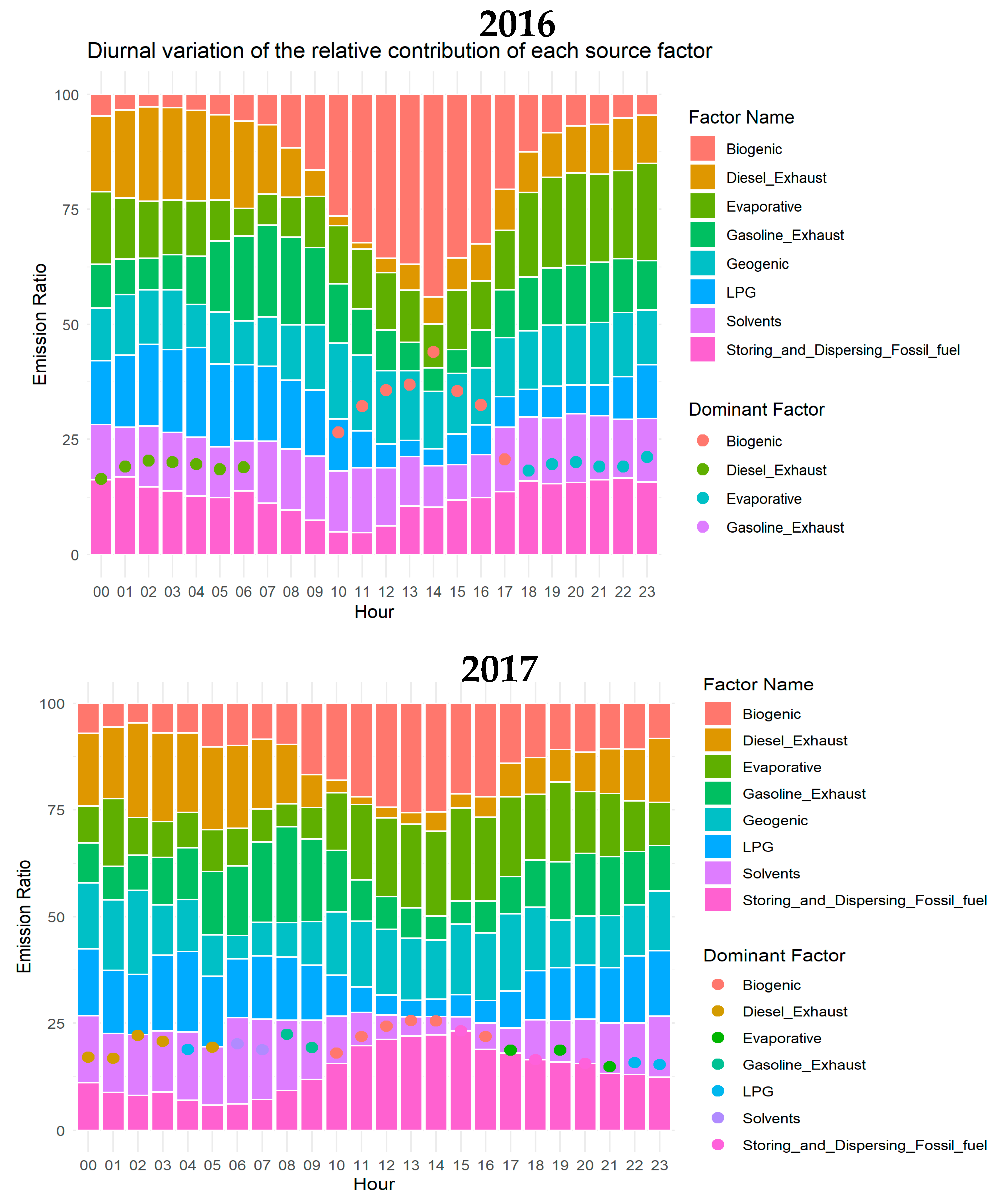
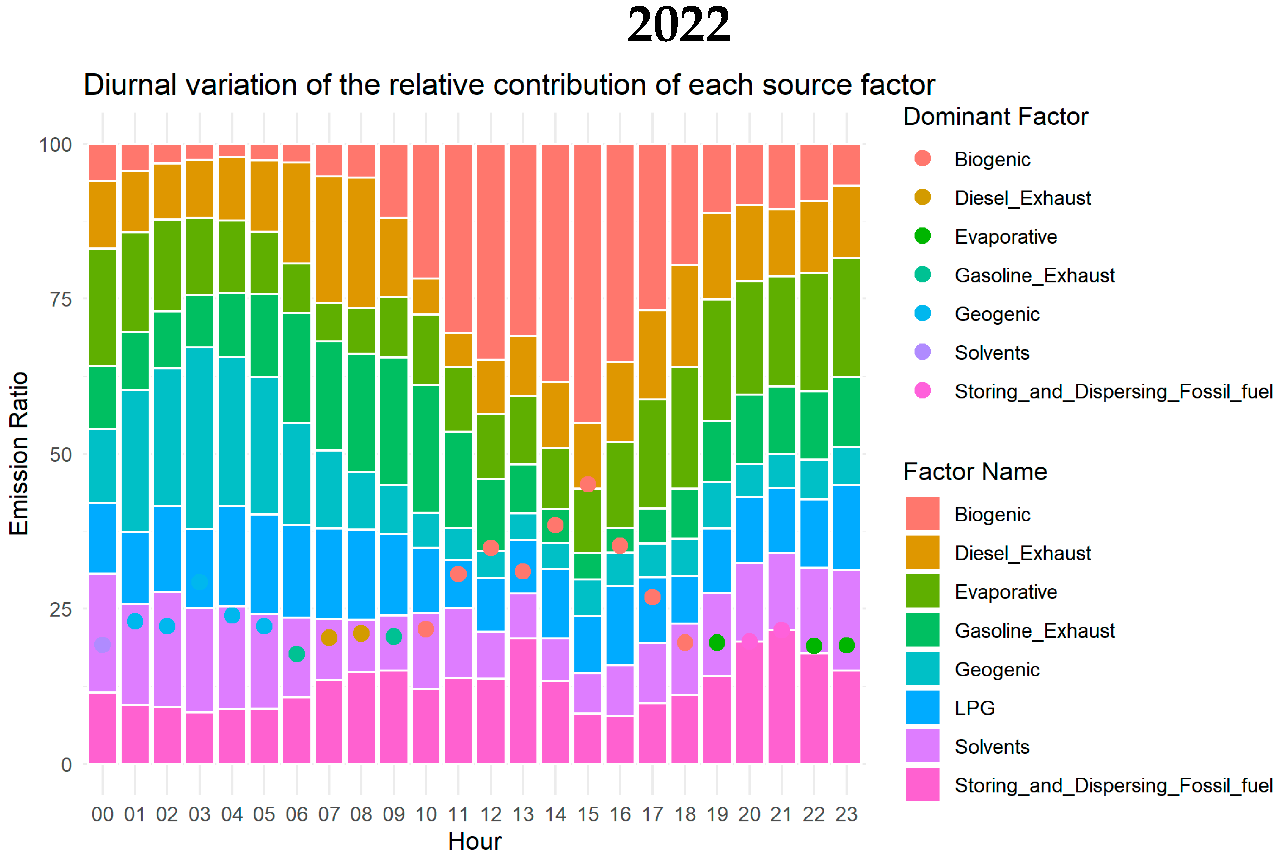
3.11. Diurnal Variations of Different Source Types

Figure 14 shows the diurnal variations of the different source types. The diurnal variation of VOC sources is influenced by physical processes, chemical reactions, emission sources, and environmental and meteorological conditions, resulting in a prominent morning peak of secondary aerosol precursors, and solvents due to traffic rush hour and the shallow boundary layer in the morning [62,85]. Biogenic emissions demonstrate a pattern showing two peaks: one morning rush hour (6:00–9:00 LT), because of traffic [59] and industrial activities [12], and another peak aligned with ambient temperature and sunlight intensity, resulting in high ambient concentrations at 13:00–15:00 LT during the day, and low emissions during the night [59,87]. The Gasoline Exhaust source factor shows one prominent peak during the morning (6:00–9:00 LT) and some slight increase later during the day (18:00–21:00 LT), whereas the diesel Exhaust source factor exclusively shows one significant peak during the morning rush hour. The LPG source shows highest contribution in the morning, which might be due to domestic cooking, whose emissions would accumulate in the shallow morning boundary layer. Notably, for the pollutant of NO2, a significant peak occurs around 11:00 LT, i.e., after the morning rush hour, which is likely associated with the buildup of this compound. The contribution of secondary aerosol precursors is higher throughout the day, indicative of the photochemical processes related to this factor. The geogenic factor exhibits a greater distribution in the morning, owing to the lower boundary layer height (BLH) and a lower contribution displayed throughout the day due to dilution processes. In the morning, the contribution of solvents is more significant compared to nighttime, due to increased industrial activity, while the BLH reaches its daytime minimum [17].

4. Interannual and Diurnal Variation

Additional VOC data sets were obtained in the subsequent years 2017, 2018, 2021, and 2022, albeit with slightly different time frames. However, all these data sets included the month of May as the 2016 data set. In order to compare similar seasonal conditions, we will focus on PMF analyses for this month for all the five years hereinafter, enabling a thorough comparative analysis. Another constraint is the focus on VOCs only, due to varying availability of ancillary pollutant data other than VOCs. The PMF profiles of source factors for each case are shown in Figures S1–S5. However, when comparing the results of the 2016 PMF analysis presented extensively in the preceding chapters with the 2016 PMF analysis for the month of May 2016 focusing on VOC data only, quite similar results were obtained (see Figure 15 and Figure S1). The PMF source factors in 2016, considering VOCs and other pollutants such as CO, NO, NO2, SO2, and PM1, share common elements with the May 2016 PMF factors when only VOCs are considered, including gasoline exhaust, diesel exhaust, LPG, solvents, geogenic, biogenic, and evaporative sources. Additionally, in the case of the PMF 2016 analysis with all pollutants, two more factors emerge: a source related to NO2 and another related to secondary aerosol precursors. On the other hand, for the PMF 2016 case with only VOCs, an additional factor is identified, associated with the storage and dispersion of fossil fuel.
The PMF analysis for the years 2016, 2017, 2018, 2021, and 2022 reveals a consistent set of common eight emission source factors across these five years (for reference see Figures S1–S5). These include contributions from gasoline and diesel exhaust, LPG, solvents, geogenic, biogenic, and evaporative emissions, as well as contributions from storage and dispersion of fossil fuel, which provides a basis for comparative analysis and understanding the contribution to air quality over this period.
The examination of the pie charts in Figure 15 elucidates consistent LPG contributions for 2017, 2021, and 2022, ranging from 23.7% to 25.4%, while the highest proportion is observed in 2016 (34.8%) and the lowest in 2018 (19.1%). Gasoline exhaust usually ranges between about 20–30% with a slight deviation in 2018 (33.5%). Diesel Exhaust contributions remain fairly consistent for 2017, 2018, 2021, and 2022, varying from 15.3% to 19.9%, with 2016 recording the lowest at 9.8%. The geogenic contribution shows little variation among the years, between 6.2% to 8.8%, with the exception of 2016, which shows slightly elevated values (12.5%). Solvents contribute similarly from 2016 and 2022, ranging from 8.6% to 10.5%, with 2021 exhibiting the lowest at 5.3%. The contribution from storing and dispersing fossil fuel is usually below 5%, but demonstrates higher proportions, ranging from 7.5% to 8 in the years 2018 and 2022, respectively. Evaporative contributions remained pretty stable through 2016–2018 (3.2–3.3%), but experienced a significant rise from 8.3% in 2021 to 9.7% in 2022. Biogenic contributions only varied slightly from 3% to 5.3% throughout the five years.
Overall, anthropogenic VOC sources accounted for about 82.2% (May 2016) to about 90.2% of the mass (May 2018). While the March–May 2016 data set analyzed in the earlier section showed somewhat higher anthropogenic source contributions (about 90%) when compared to the analysis restricted to May 2016, it should be noted that the May 2016 PMF analysis focused on VOCs only and also yielded some variations in the sources. The May 2016 VOC PMF results can be considered as a lower limit for anthropogenic VOCs, which needs to be accounted for in emission control policies. Major anthropogenic VOC source contributions come from LPG, gasoline and Diesel exhaust, with altogether 60.3–72.8% throughout the five years.
Figure 16 provides a detailed insight into the diurnal variations of relative contribution of the different emission source factors, which eliminates potential impacts of diurnal variations of the BLH as prevalent in Figure 14. In the following discussion we split the day into four time windows: (I) early morning before sunrise (0:00–6:00 LT) which is usually characterized by lowest wind speeds [29] and low stable nocturnal BLHs [17], (II) the morning rush hour (6:00–9:00 LT) when the highest traffic volume occurs, while the BLH is either at its daytime minimum and/or on the decrease, but the residual layer contents has not yet been mixed with the surface layer, (III) the daytime (9:00–18:00 LT), when solar radiation is present [29], the daytime atmospheric mixing is highest and the convective boundary layer fully developed with maximum BLH [17], and (IV) the evening hours after sunset (18:00–23:00 LT), when the surface boundary layer starts to develop and decouples from the residual layer aloft [17].
Figure 16 indicates the dominant source contributions for each hour. They may change from hour to hour, when source contributions are of similar magnitude and would not differ much, but for other hours, the dominating source signals may be prevalent for several consecutive hours, if not for the entire time window. In general dominant source contributions in the early morning hours (0:00–6:00 LT) originate from four sources: solvent, evaporative, geogenic, and diesel exhaust emissions, with varying contributions from hour to hour and year to year, but mostly between 12–25% each. The first three sources have in common that these are usually continuously emitting area sources which eventually will accumulate in the shallow nocturnal boundary layer. Their emission strength also depends on the ambient temperature and this may explain the temporal variability. Diesel exhaust is closely tied to heavy duty vehicles and is mostly linked to distribution of merchandise within Mexico City, as well as transportation from outside into the city in these early hours [29].
During rush hours (6:00–9:00 LT), combustion related emissions, as well as the storing and dispersing of fossil fuel, are the most important VOC emission sources. While their contributions also do vary from hour to hour and year to year, it should be noted that each source can reach high contributions of more than 20% each, with maximum values of 27% for storing and dispersing of fossil fuel (2017) and 28% for diesel exhaust (2021). Interestingly, storing and dispersing fossil fuel is even the dominant source in 2016, 2017, and 2021 during the rush hours, which should be considered in emission control strategies. As mentioned earlier, this rush hour time window is usually associated with low horizontal and vertical atmospheric mixing, making it a critical time in photochemical process that start after sunrise.
As can be expected, biogenic emissions are largely dominating during daytime (9:00–18:00 LT) throughout the five years, with 25–48%, as biogenic emissions are known to be triggered by solar radiation and temperature, even more in the month of May. Nevertheless, still diesel exhaust and fossil fuel storage and dispersing can reach appreciable values of more than 20% in some years and rank among the next important VOC emission sources during daytime.
In the evening hours (18:00–23:00 LT), i.e., after sunset, with developing of a stable surface boundary layer, VOC emission sources which are among the prevalent sources in the morning hours gain importance again. These include evaporative and geogenic emissions, with about 20–25% each. Apart from those, also fossil fuel storage and dispersion is important at times (about 20–22%), and also biogenic emissions can still be appreciable (up to 26% in 2017), which is different from early morning hours. The latter two sources also depend on temperature, and temperatures are still higher in the evening hours compared to early morning hours, which can explain these differences.

5. Atmospheric Implications

The abundance of VOCs in the atmosphere is determined by emissions, transport processes, chemical transformations, and ultimately removal processes through deposition processes (also through SOA formation), which largely depend on the volatility and solubility properties of the specific VOC. In addition, boundary layer variations modulate the diurnal variation of VOC concentrations in the lower atmosphere. Daytime photochemical transformation processes of VOCs, mostly with OH, but also O3, lead to the formation of O3 and SOA, as outlined in the Introduction section. Nighttime chemistry involves NO3 reactions with selected VOCs, e.g., isoprene, 1.3-butadiene and i-butene [88], and can alter the NOx and VOC budget. Cl radicals would react with VOCs, regardless of the daytime. However, these radicals are more prevalent in coastal areas and/or are related to specific industrial activities. With regard to O3 formation potentials in the MCMA, [29] found that most important individual VOCs include the alkenes ethylene and propylene, the aromatics m/p-xylene and toluene, and also isoprene. The most important alkane is propane, mostly due to its high abundance. Most important sources for these VOCs include gasoline and diesel exhaust (e.g., for ethylene and aromatics), LPG (for propane), solvents (for aromatics), and biogenic (and exhaust) sources for isoprene. While some of these sources are prominent in specific time frames (e.g., rush hour), some are related to broader daytime activities (e.g., LPG, solvents) and some also depend on the ambient temperature (solvents) or solar radiation (biogenic isoprene emissions). Each of these emissions would have varying contributions to O3 and SOA formation during the daytime, depending on its abundance and reactivity.

6. Policy Regulations

Our results show that anthropogenic VOC emissions account to about 80–90% of the total VOC mass and implies that regulating VOC emissions is critical. [29] used boundary layer height data to normalize pollutant concentration. This work revealed that photochemical processes were maintained for an appreciable period of time extending into the late afternoon. This is due to ongoing emissions, accumulation, but also due to recirculation processes which occur in the basin of MCMA during severe O3 episodes. [29] suggested modified O3 mitigation strategies which would focus on specific time periods during the day. This included disentangling traffic flows considering different work and school times and on the other hand, moving heavy-duty vehicle transport to other time slots when photochemical processes are slowing down or at a minimum (e.g., afternoon or night). Our findings suggest that, additionally, emission sources which also depend on ambient temperature should be reduced in particular during the time of the day when highest temperatures occur. This would include the emissions of solvents (e.g., for the use of painting, etc.), for instance. This would be important as those are the times of the day, when biogenic isoprene emissions tend to reach the daytime maximum.

7. Conclusions

Our study employed hourly measurements of VOCs, NO, NO2, CO, SO2, and PM1, to identify potential sources in Mexico City during the ozone season from March to May 2016. Compared to earlier studies, we utilized data from these months to derive a more robust source apportionment solution using the Positive Matrix Factorization (PMF) and applied bivariate plots to locate potential emission source areas. Our analysis revealed a total of nine sources, including secondary aerosol precursors (21.7%), NO2 (20.4%), Gasoline Exhaust (19.3%), Diesel Exhaust (16.2%), LPG (7.3%), geogenic (5.3%), biogenic (4.8%), Evaporative (2.7%), and solvents (2.3%). Our results show that anthropogenic VOC emissions account for about 80–90% of the total VOC mass. Natural sources, like biogenic and geogenic sources, play a marginal, albeit non-negligible role. Biogenic emissions tend to become more important towards the end of the ozone season. However, isoprene, can be found in traffic emissions throughout the ozone season. Our analysis confirms a geogenic source factor throughout the three months measurement period, which confirms earlier suggestions by [29] based on a short-term analysis. This factor is low in magnitude and based on the major components i-pentane and pentane, likely much less reactive than isoprene in the biogenic source factor.
In an extended study focusing on VOC data obtained in the months of May of the years 2016, 2017, 2018, 2021, and 2022, interannual and diurnal variations of VOC sources were obtained. The PMF results revealed eight emission factors: gasoline and diesel exhaust, LPG, solvents, geogenic, biogenic, and evaporative emissions, as well as contributions from storage and dispersion of fossil fuel. Major anthropogenic VOC source contributions come from LPG, gasoline and diesel exhaust, with 60.3–72.8% in total through the five years.
The analysis of the diurnal variation of the relative contribution of each emission factor showed that, in general, continuously emitting area sources are dominant at night times. These include solvent, evaporative, and geogenic emissions in the early morning hours (00:00–6:00 LT), while during the evening hours (18:00–23:00 LT) biogenic emissions and emissions from fossil fuel storage and dispersion may also contribute appreciably. All these sources have in common that they are temperature dependent. Apart from these sources, diesel exhaust can contribute substantially during the morning hours due to heavy-duty trucks for distributing merchandise. During rush hours (6:00–9:00 LT) combustion related emissions as well as storing and dispersing of fossil fuel are the most important VOC emission sources. Biogenic emissions dominate during daytime (9:00–18:00 LT) in all the five years. Apart from biogenic emissions, diesel exhaust and fossil fuel storage and dispersing rank among the next important VOC emission sources during daytime.
Our spatiotemporal variability analysis of identified VOC sources provides valuable insights for evaluating and optimizing emission control policies and effective strategies to reduce ambient VOC concentrations.

Supplementary Materials

The following supporting information can be downloaded at: https://www.mdpi.com/article/10.3390/atmos15020179/s1, Figure S1: Profiles of source factors determined for VOCs by PMF for the month of May 2016; Figure S2: Profiles of source factors determined for VOCs by PMF for the month of May 2017; Figure S3: Profiles of source factors determined for VOCs by PMF for the month of May 2018; Figure S4: Profiles of source factors determined for VOCs by PMF for the month of May 2021; Figure S5: Profiles of source factors determined for VOCs by PMF for the month of May 2022; Table S1: Summary of PMF runs for seven, eight, and nine-factor solutions; Table S2: Bootstrap analysis results for 9 factors (F) solution based on 20 bootstrap runs; Table S3: Statistical parameters for VOCs, NO, NO2, CO, and SO2. VOCs are ordered according to their elution in the gas chromatogram. Data in ppb for VOCs, NO, NOx, CO, SO2 and μg/m3 for PM1.

Author Contributions

M.J.A.: Methodology, Formal analysis, PMF Software, openair package software, Writing—original draft; B.R.: Conceptualization, Methodology, Formal analysis, Writing—review and editing; A.R.: resources, data curation, review and editing. O.R.-H.: resources, data curation. All authors have read and agreed to the published version of the manuscript.

Funding

The authors appreciate the project Ozone Precursors Monitoring Campaign funded by the Fondo Ambiental Público del Distrito Federal (FAP) Agreement EXT 49.09.16.

Institutional Review Board Statement

Not applicable.

Informed Consent Statement

Not applicable.

Data Availability Statement

The original contributions presented in the study are included in the article and Supplementary Materials, further inquiries can be directed to the corresponding authors.

Acknowledgments

The authors acknowledge the Sistema de Monitoreo Atmosférico (SIMAT) for providing air quality data.

Conflicts of Interest

The authors declare no conflicts of interest.

References

  1. Bari, M.A.; Kindzierski, W.B.; Spink, D. Twelve-year trends in ambient concentrations of volatile organic compounds in a community of the Alberta Oil Sands Region, Canada. Environ. Int. 2016, 91, 40–50. [Google Scholar] [CrossRef] [PubMed]
  2. Ma, Z.; Liu, C.; Zhang, C.; Liu, P.; Ye, C.; Xue, C.; Zhao, D.; Sun, J.; Du, Y.; Chai, F. The levels, sources, and reactivity of volatile organic compounds in a typical urban area of Northeast China. J. Environ. Sci. 2019, 79, 121–134. [Google Scholar] [CrossRef] [PubMed]
  3. Claeys, M.; Graham, B.; Vas, G.; Wang, W.; Vermeylen, R.; Pashynska, V.; Cafmeyer, J.; Guyon, P.; Andreae, M.O.; Artaxo, P. Formation of secondary organic aerosols through photooxidation of isoprene. Science 2004, 80, 1173–1176. [Google Scholar] [CrossRef] [PubMed]
  4. Louie, P.K.K.; Ho, J.W.K.; Tsang, R.C.W.; Blake, D.R.; Lau, A.K.H.; Yu, J.Z.; Yuan, Z.B.; Wang, X.M.; Shao, M.; Zhong, L.J. VOCs and OVOCs distribution and control policy implications in Pearl River Delta region, China. Atmos. Environ. 2013, 76, 125–135. [Google Scholar] [CrossRef]
  5. Tham, Y.J.; Wang, Z.; Li, Q.; Yun, H.; Wang, W.; Wang, X.; Xue, L.; Lu, K.; Ma, N.; Bohn, B. Significant concentrations of nitryl chloride sustained in the morning: Investigations of the causes and impacts on ozone production in a polluted region of northern China. Atmos. Chem. Phys. 2016, 16, 14959–14977. [Google Scholar] [CrossRef]
  6. Atkinson, R.; Arey, J. Atmospheric degradation of volatile organic compounds. Chem. Rev. 2003, 103, 4605–4638. [Google Scholar] [CrossRef] [PubMed]
  7. Schauer, J.J.; Fraser, M.P.; Cass, G.R.; Simoneit, B.R.T. Source reconciliation of atmospheric gas phase and particle-phase pollutants during a severe photochemical smog episode. Environ. Sci. Technol. 2002, 36, 3806–3814. [Google Scholar] [CrossRef]
  8. Yuan, B.; Hu, W.W.; Shao, M.; Wang, M.; Chen, W.T.; Lu, S.H.; Zeng, L.M.; Hu, M. VOC emissions, evolutions and contributions to SOA formation at a receptor site in Eastern China. Atmos. Chem. Phys. Discuss. 2013, 13, 6631–6679. [Google Scholar] [CrossRef]
  9. McFiggans, G.; Mentel, T.F.; Wildt, J.; Pullinen, I.; Kang, S.; Kleist, E.; Schmitt, S.; Springer, M.; Tillmann, R.; Wu, C. Secondary organic aerosol reduced by mixture of atmospheric vapours. Nature 2019, 565, 587–593. [Google Scholar] [CrossRef]
  10. Rumchev, K.; Brown, H.; Spickett, J. Volatile organic compounds: Do they present a risk to our health? Rev. Environ. Health 2007, 22, 39–56. [Google Scholar] [CrossRef]
  11. Azuma, K.; Uchiyama, I.; Uchiyama, S.; Kunugita, N. Assessment of inhalation exposure to indoor air pollutants: Screening for health risks of multiple pollutants in Japanese dwellings. Environ. Res. 2016, 145, 39–49. [Google Scholar] [CrossRef]
  12. McCarthy, M.C.; O’Brien, T.E.; Charrier, J.G.; Hafner, H.R. Characterization of the chronic risk and hazard of hazardous air pollutants in the United States using ambient monitoring data. Environ. Health Perspect. 2009, 117, 790–796. [Google Scholar] [CrossRef] [PubMed]
  13. U.S. Environmental Protection Agency, 2011. 2005 National-Scale Air Toxics Assessment. Available online: http://www.epa.gov/nata2005/ (accessed on 21 September 2023).
  14. Kim, H.Y.; Lee, J.D.; Kim, J.Y.; Lee, J.Y.; Bae, O.N.; Choi, Y.K.; Baek, E.; Kang, S.; Min, C.; Seo, K. Risk assessment of volatile organic compounds (VOCs) detected in sanitary pads. J. Toxicol. Environ. Health Part A 2019, 82, 678–695. [Google Scholar] [CrossRef] [PubMed]
  15. Lei, W.; de Foy, B.; Zavala, M.; Volkamer, R.; Molina, L.T. Characterizing ozone production in the Mexico City Metropolitan Area: A case study using a chemical transport model. Atmos. Chem. Phys. 2007, 7, 1347–1366. [Google Scholar] [CrossRef]
  16. Molina, L.T.; Molina, M.J. (Eds.) Air Quality in the Mexico Megacity: An Integrated Assessment; Kluwer Academic Publishers: Dordrecht, The Netherlands, 2002; 390p. [Google Scholar]
  17. Osibanjo, O.O.; Rappenglück, B.; Retama, A. Anatomy of the March 2016 Severe Ozone Smog Episode in Mexico-City. Atmos. Environ. 2021, 244, 117945. [Google Scholar] [CrossRef]
  18. Jaimes-Palomera, M.; Retama, A.; Elias-Castro, G.; Neria-Hernández, A.; Rivera-Hernández, O.; Velasco, E. Non-methane hydrocarbons in the atmosphere of Mexico City: Results of the 2012 ozone-season campaign. Atmos. Environ. 2016, 132, 258–275. [Google Scholar] [CrossRef]
  19. Tie, X.; Madronich, S.; Li, G.; Ying, Z.; Zhang, R.; Garcia, A.R.; Lee-Taylor, J.; Liu, Y. Characterizations of chemical oxidants in Mexico City: A regional chemical dynamical model (WRF-Chem) study. Atmos. Environ. 2007, 41, 1989–2008. [Google Scholar] [CrossRef]
  20. Zavala, M.; Brune, W.H.; Velasco, E.; Retama, A.; Cruz-Alavez, L.A.; Molina, L.T. Changes in ozone production and VOC reactivity in the atmosphere of the Mexico City Metropolitan Area. Atmos. Environ. 2020, 238, 117747. [Google Scholar] [CrossRef]
  21. SEDEMA, 2021. Inventario de Emisiones de la Zona Metropolitana del Valle de Mexico 2018. In Secretaría del Medio Ambiente de la Ciudad de Mexico Direction General de Calidad del Aire; Direction de Proyectos de Calidad del Aire: Ciudad de Mexico, Agosto 2021; Available online: https://www.sedema.cdmx.gob.mx/storage/app/media/DGCA/InventarioDeEmisionesZMVM2018.pdf (accessed on 21 September 2023).
  22. Vega, E.; Mugica, V.; Carmona, C.; Valencia, E. Hydrocarbon source apportionment in Mexico City using the chemical mass balance receptor model. Atmos. Environ. 2000, 34, 4121–4129. [Google Scholar] [CrossRef]
  23. Mugica, V.; Watson, J.; Vega, E.; Reyes, E.; Ruiz, M.E.; Chow, J. Receptor model source apportionment of nonmethane hydrocarbons in Mexico City. Sci. World J. 2002, 2, 844–860. [Google Scholar] [CrossRef]
  24. Velasco, E.; Márquez, C.; Bueno, E.; Bernabé, R.M.; Sánchez, A.; Fentanes, O.; Wöhrnschimmel, H.; Cárdenas, B.; Kamilla, A.; Wakamatsu, S. Vertical distribution of ozone and VOCs in the low boundary layer of Mexico City. Atmos. Chem. Phys. 2008, 8, 3061–3079. [Google Scholar] [CrossRef]
  25. Wöhrnschimmel, H.; Magaña, M.; Stahel, W.A.; Blanco, S.; Acuna, S.; Pérez, J.M.; González, S.; Gutiérrez, V.; Wakamatsu, S.; Cárdenas, B. Measurements and receptor modeling of volatile organic compounds in Southeastern Mexico City, 2000–2007. Atmos. Chem. Phys. 2010, 10, 9027–9037. [Google Scholar] [CrossRef]
  26. Vega, E.; Ramírez, O.; Sánchez-Reyna, G.; Chow, J.C.; Watson, J.G.; López-Veneroni, D.; Jaimes-Palomera, M. Volatile Organic Compounds and Carbonyls Pollution in Mexico City and an Urban Industrialized Area of Central Mexico. Aerosol Air Qual. Res. 2022, 22, 210386. [Google Scholar] [CrossRef]
  27. SEMARNAT, 2008. Capítulo 5. Atmósfera. Available online: https://www.yumpu.com/es/document/view/14860837/capitulo-5-atmosfera-semarnat (accessed on 21 September 2023).
  28. SEDEMA, 2013. Secretaría del Medio Ambiente. Available online: http://data.sedema.cdmx.gob.mx/sedema/images/archivos/noticias/primer-informe-sedema/portada-indice.pdf (accessed on 21 September 2023).
  29. Akther, T.; Rappenglueck, B.; Osibanjo, O.; Retama, A.; Rivera-Hernández, O. Ozone precursors and boundary layer meteorology before and during a severe ozone episode in Mexico-City. Chemosphere 2023, 318, 137978. [Google Scholar] [CrossRef] [PubMed]
  30. Mejía-Ponce, L.V.; Hernández-López, A.E.; Miranda-Martín-del-Campo, J.; Pineda-Santamaría, J.C.; Reynoso-Cruces, S.; Mendoza-Flores, J.A.; Espinosa-Guzmán, A.A. Elemental analysis of PM10 in southwest Mexico City and source apportionment using positive matrix factorization. J. Atmos. Chem. 2022, 79, 167–198. [Google Scholar] [CrossRef]
  31. Lee, S.; Liu, W.; Wang, Y.; Russell, A.G.; Edgerton, E.S. Source apportionment of PM2.5: Comparing PMF and CMB results for four ambient monitoring sites in the southeastern United States. Atmos. Environ. 2008, 42, 4126–4137. [Google Scholar] [CrossRef]
  32. Watson, J.G.; Antony Chen, L.W.; Chow, J.C.; Doraiswamy, P.; Lowenthal, D.H. Source apportionment: Findings from the US supersites program. J. Air Waste Manag. Assoc. 2008, 58, 265–288. [Google Scholar] [CrossRef] [PubMed]
  33. Cesari, D.; Donateo, A.; Conte, M.; Contini, D. Inter-comparison of source apportionment of PM10 using PMF and CMB in three sites nearby an industrial area in central Italy. Atmos. Res. 2016, 182, 282–293. [Google Scholar] [CrossRef]
  34. Hopke, P.K. The application of receptor modeling to air quality data. Pollut. Atmosphérique 2010, (SEP), 91–109. Available online: https://www.appa.asso.fr/wp-content/uploads/2020/02/Hopke_2010.pdf (accessed on 21 September 2023).
  35. Norris, G.; Duvall, R.; Brown, S.; Bai, S. EPA Positive Matrix Factorization (PMF) 5.0 Fundamentals and User Guide; EPA/600/R-14/108; STI-910511-5594-UG, April; U.S. Environmental Protection Agency Office of Research and Development: Washington, DC, USA, 2014.
  36. Paatero, P.; Tapper, U. Positive matrix factorization: A non-negative factor model with optimal utilization of error estimates of data values. Environmetrics 1994, 5, 111–126. [Google Scholar] [CrossRef]
  37. Paatero, P. Least squares formulation of robust non-negative factor analysis. Chemom. Intell. Lab. Syst. 1997, 37, 23–35. [Google Scholar] [CrossRef]
  38. Paatero, P.; Eberly, S.; Brown, S.G.; Norris, G.A. Methods for estimating uncertainty in factor analytic solutions. Atmos. Meas. Tech. 2014, 7, 781. [Google Scholar] [CrossRef]
  39. Ahmed, M.; Rappenglück, B.; Das, S.; Chellam, S. Source apportionment of volatile organic compounds, CO, SO2 and trace metals in a complex urban atmosphere. Environ. Adv. 2021, 6, 10012. [Google Scholar] [CrossRef]
  40. Bozlaker, A.; Buzcu-Güven, B.; Fraser, M.P.; Chellam, S. Insights into PM10 sources in Houston, Texas: Role of petroleum refineries in enriching lanthanoid metals during episodic emission events. Atmos. Environ. 2013, 69, 109–117. [Google Scholar] [CrossRef]
  41. Ahmed, M.; Rappenglueck, B.; Ganranoo, L.; Dasgupta, P.K. Source apportionment of gaseous Nitrophenols and their contribution to HONO formation in an urban area. Chemosphere 2023, 338, 139499. [Google Scholar] [CrossRef] [PubMed]
  42. Carslaw, D.C.; Beevers, S.D. Characterising and understanding emission sources using bivariate polar plots and k-means clustering. Environ. Model. Softw. 2013, 40, 325–329. [Google Scholar] [CrossRef]
  43. Carslaw, D.C.; Ropkins, K. Openair—An R package for air quality data analysis. Environ. Model. Softw. 2012, 27, 52–61. [Google Scholar] [CrossRef]
  44. Wood, S.N. Generalized Additive Models: An Introduction with R.; International Standard Book Number-13:978-1-4987-2833-1; CRC Press: Boca Raton, FL, USA, 2017. [Google Scholar]
  45. Henry, R.; Norris, G.A.; Vedantham, R.; Turner, J.R. Source region identification using kernel smoothing. Environ. Sci. Technol. 2009, 43, 4090–4097. [Google Scholar] [CrossRef] [PubMed]
  46. Fuentes, J.D.; Lerdau, M.; Atkinson, R.; Baldocchi, D.; Bottenheim, J.W.; Ciccioli, P.; Lamb, B.; Geron, C.; Gu, L.; Guenther, A. Biogenic hydrocarbons in the atmospheric boundary layer: A review. Bull. Amer. Meteor. Soc. 2000, 81, 1537–1575. [Google Scholar] [CrossRef]
  47. Guenther, A. Seasonal and spatial variations in natural volatile organic compound emissions. Ecol. Appl. 1997, 7, 34–45. [Google Scholar] [CrossRef]
  48. Guenther, A. Review of the Effects of Drought and High Temperature on Biogenic Emissions. 2001. Available online: http://www.tceq.state.tx.us/assets/public/implementation/air/am/contracts/reports/ei/EffectsOfDroughtHighTemperatureOnBiogenicEmissions.pdf (accessed on 13 September 2023).
  49. Reimann, S.; Calanca, P.; Hofer, P. The anthropogenic contribution to isoprene concentrations in a rural atmosphere. Atmos. Environ. 2000, 34, 109–115. [Google Scholar] [CrossRef]
  50. Borbon, A.; Fontaine, H.; Veillerot, M.; Locoge, N.; Galloo, J.C.; Guillermo, R. An investigation into the traffic-related fraction of isoprene at an urban location. Atmos. Environ. 2001, 35, 3749–3760. [Google Scholar] [CrossRef]
  51. Diskin, A.M.; Španěl, P.; Smith, D. Time variation of ammonia, acetone, isoprene and ethanol in breath: A quantitative SIFT-MS study over 30 days. Physiol. Meas. 2003, 24, 107. [Google Scholar] [CrossRef] [PubMed]
  52. Kinoyama, M.; Nitta, H.; Watanabe, A.; Ueda, H. Acetone and isoprene concentrations in exhaled breath in healthy subjects. J. Health Sci. 2008, 54, 471–477. [Google Scholar] [CrossRef]
  53. Veres, P.R.; Faber, P.; Drewnick, F.; Lelieveld, J.; Williams, J. Anthropogenic sources of VOC in a football stadium: Assessing human emissions in the atmosphere. Atmos. Environ. 2013, 77, 1052–1059. [Google Scholar] [CrossRef]
  54. Wagner, P.; Kuttler, W. Biogenic and anthropogenic isoprene in the near-surface urban atmosphere—A case study in Essen. Germany. Sci. Total Environ. 2014, 475, 104–115. [Google Scholar] [CrossRef] [PubMed]
  55. Molina, L.T.; Kolb, C.E.; De Foy, B.; Lamb, B.K.; Brune, W.H.; Jimenez, J.L.; Ramos-Villegas, R.; Sarmiento, J.; Paramo-Figueroa, V.H.; Cardenas, B. Air quality in North America’s most populous city–overview of the MCMA-2003 campaign. Atmos. Chem. Phys. 2007, 7, 2447–2473. [Google Scholar] [CrossRef]
  56. Molina, L.T.; Madronich, S.; Gaffney, J.S.; Apel, E.; de Foy, B.; Fast, J.; Ferrare, R.; Herndon, S.; Jimenez, J.L.; Lamb, B. An overview of the MILAGRO 2006 Campaign: Mexico City emissions and their transport and transformation. Atmos. Chem. Phys. 2010, 10, 8697–8760. [Google Scholar] [CrossRef]
  57. Velasco, E.; Lamb, B.; Westberg, H.; Allwine, E.; Sosa, G.; Arriaga-Colina, J.L.; Jobson, B.T.; Alexander, M.L.; Prazeller, P.; Knighton, W.B. Distribution, magnitudes, reactivities, ratios and diurnal patterns of volatile organic compounds in the Valley of Mexico during the MCMA 2002 & 2003 field campaigns. Atmos. Chem. Phys. 2007, 7, 329–353. [Google Scholar] [CrossRef]
  58. Bon, D.M.; Ulbrich, I.M.; De Gouw, J.A.; Warneke, C.; Kuster, W.C.; Alexander, M.L.; Baker, A.; Beyersdorf, A.J.; Blake, D.; Fall, R. Measurements of volatile organic compounds at a suburban ground site (T1) in Mexico City during the MILAGRO 2006 campaign: Measurement comparison, emission ratios, and source attribution. Atmos. Chem. Phys. 2011, 11, 2399–2421. [Google Scholar] [CrossRef]
  59. Velasco, E. Estimates for biogenic non-methane hydrocarbons and nitric oxide emissions in the Valley of Mexico. Atmos. Environ. 2003, 37, 625–637. [Google Scholar] [CrossRef]
  60. Sharkey, T.D.; Wiberley, A.E.; Donohue, A.R. Isoprene emission from plants: Why and how. Ann. Bot. 2008, 101, 5–18. [Google Scholar] [CrossRef]
  61. Staehelin, J.; Schläpfer, K.; Bürgin, T.; Steinemann, U.; Schneider, S.; Brunner, D.; Bäumle, M.; Meier, M.; Zahner, C.; Keiser, S. Emission factors from road traffic from a tunnel study (Gubrist tunnel, Switzerland). Part I: Concept and first results. Sci. Total Environ. 1995, 169, 141–147. [Google Scholar] [CrossRef]
  62. Leuchner, M.; Rappenglück, B. VOC source–receptor relationships in Houston during TexAQS-II. Atmos. Environ. 2010, 44, 4056–4067. [Google Scholar] [CrossRef]
  63. Gurjar, B.R.; Ravindra, K.; Nagpure, A.S. Air pollution trends over Indian megacities and their local-to-global implications. Atmos. Environ. 2016, 142, 475–495. [Google Scholar] [CrossRef]
  64. Jain, S.; Aggarwal, P.; Sharma, P.; Kumar, P. Vehicular exhaust emissions under current and alternative future policy measures for megacity Delhi, India. J. Transp. Health 2016, 3, 404–412. [Google Scholar] [CrossRef]
  65. Orun, A.; Elizondo, D.; Goodyer, E.; Paluszczyszyn, D. Use of Bayesian inference method to model vehicular air pollution in local urban areas. Transp. Res. Part D Transp. Environ. 2018, 63, 236–243. [Google Scholar] [CrossRef]
  66. Nakashima, Y.; Sadanaga, Y.; Saito, S.; Hoshi, J.; Ueno, H. Contributions of vehicular emissions and secondary formation to nitrous acid concentrations in ambient urban air in Tokyo in the winter. Sci. Total Environ. 2017, 592, 178–186. [Google Scholar] [CrossRef]
  67. Fujita, E.M.; Croes, B.E.; Bennett, C.L.; Lawson, D.R.; Lurmann, F.W.; Main, H.H. Comparison of emission inventory and ambient concentration ratios of CO, NMOG, and NOx in California’s South Coast Air Basin. J. Air Waste Manag. Assoc. 1992, 42, 264–276. [Google Scholar] [CrossRef]
  68. Parrish, D.D.; Trainer, M.; Hereid, D.; Williams, E.J.; Olszyna, K.J.; Harley, R.A.; Meagher, J.F.; Fehsenfeld, F.C. Decadal change in carbon monoxide to nitrogen oxide ratio in US vehicular emissions. J. Geophys. Res. Atmos. 2002, 107, ACH-5. [Google Scholar] [CrossRef]
  69. Parrish, D.D. Critical evaluation of US on-road vehicle emission inventories. Atmos. Environ. 2006, 40, 2288–2300. [Google Scholar] [CrossRef]
  70. Blake, D.R.; Rowland, F.S. Urban leakage of liquefied petroleum gas and its impact on Mexico City air quality. Science 1995, 269, 953–956. [Google Scholar] [CrossRef]
  71. Garzón, J.P.; Huertas, J.I.; Magaña, M.; Huertas, M.E.; Cárdenas, B.; Watanabe, T.; Maeda, T.; Wakamatsu, S.; Blanco, S. Volatile organic compounds in the atmosphere of Mexico City. Atmos. Environ. 2015, 119, 415–429. [Google Scholar] [CrossRef]
  72. Gamas, E.D.; Magdaleno, M.; Diaz, L.; Schifter, I.; Ontiveros, L.; Alvarez-Cansino, G. Contribution of liquefied petroleum gas to air pollution in the metropolitan area of Mexico City. J. Air Waste Manag. Assoc. 2000, 50, 188–198. [Google Scholar] [CrossRef] [PubMed]
  73. Tsai, D.H.; Wang, J.L.; Wang, C.H.; Chan, C.C. A study of ground-level ozone pollution, ozone precursors and subtropical meteorological conditions in central Taiwan. J. Environ. Monit. 2008, 10, 109–118. [Google Scholar] [CrossRef] [PubMed]
  74. Han, X.; Naeher, P.L. A review of traffic-related air pollution exposure assessment studies in the developing world. Environ. Int. 2006, 32, 106–120. [Google Scholar] [CrossRef] [PubMed]
  75. Koppmann, R. (Ed.) Volatile Organic Compounds in the Atmosphere; John Wiley & Sons: Hoboken, NJ, USA, 2008. [Google Scholar]
  76. Sadeghi, B.; Pouyaei, A.; Choi, Y.; Rappenglueck, B. Influence of seasonal variability on source characteristics of VOCs at Houston industrial area. Atmos. Environ. 2022, 277, 119077. [Google Scholar] [CrossRef]
  77. Chen, T.; Zhang, P.; Chu, B.; Ma, Q.; Ge, Y.; Liu, J.; He, H. Secondary organic aerosol formation from mixed volatile organic compounds: Effect of RO2 chemistry and precursor concentration. npj Clim. Atmos. Sci. 2022, 5, 95. [Google Scholar] [CrossRef]
  78. Guzy, P.; Pietrzycki, D.; Świerczewska, A.; Sechman, H.; Twaróg, A.; Góra, A. Emission Measurements of Geogenic Greenhouse Gases in the Area of “Pusty Las” Abandoned Oilfield (Polish Outer Carpathians). J. Ecol. Eng. 2017, 18, 100–109. [Google Scholar] [CrossRef] [PubMed]
  79. Wheatley, R.; Hackett, C.; Bruce, A.; Kundzewicz, A. Effect of substrate composition on production of volatile organic compounds from Trichoderma spp. inhibitory to wood decay fungi. Int. Biodeterior. Biodegrad. 1997, 39, 199–205. [Google Scholar] [CrossRef]
  80. Insam, H.; Seewald, M.S. Volatile organic compounds (VOCs) in soils. Biol. Fertil 2010, 46, 199–213. [Google Scholar] [CrossRef]
  81. Rossabi, S.; Choudoir, M.; Helmig, D.; Hueber, J.; Fierer, N. Volatile organic compound emissions from soil following wetting events. J. Geophys. Res. Biogeosci. 2018, 123, 1988–2001. [Google Scholar] [CrossRef]
  82. Lu, X.; Ma, Z.; Yi, L.; Zhang, G.; Chen, F.; Han, F. The composition and distribution of volatile organic compounds in sediments of the East Taijinar salt lake in Northern Qinghai-Tibet Plateau. Front. Environ. Chem. 2021, 2, 653867. [Google Scholar] [CrossRef]
  83. Mo, Z.; Lu, S.; Li, Y.; Shao, M.; Qu, H. Emission characteristics of volatile organic compounds (VOCs) from typical solvent use factories in Beijing. China Environ. Sci. 2015, 35, 374–380. [Google Scholar] [CrossRef]
  84. Xiong, Y.; Bari, M.A.; Xing, Z.; Du, K. Ambient volatile organic compounds (VOCs) in two coastal cities in western Canada: Spatiotemporal variation, source apportionment, and health risk assessment. Sci. Total Environ. 2020, 706, 135970. [Google Scholar] [CrossRef] [PubMed]
  85. Li, B.; Ho, S.S.H.; Gong, S.; Ni, J.; Li, H.; Han, L.; Yang, Y.; Qi, Y.; Zhao, D. Characterization of VOCs and their related atmospheric processes in a central Chinese city during severe ozone pollution periods. Atmos. Chem. Phys. 2019, 19, 617–638. [Google Scholar] [CrossRef]
  86. Mugica, V.; Ruiz, M.E.; Watson, J.; Chow, J. Volatile aromatic compounds in Mexico City atmosphere: Levels and source apportionment. Atmosfera 2003, 16, 15–27. [Google Scholar]
  87. Guenther, A.B.; Zimmerman, P.R.; Harley, P.C.; Monson, R.K.; Fall, R. Isoprene and monoterpene emission rate variability: Model evaluations and sensitivity analyses. J. Geophys. Res. Atmos. 1993, 98, 12609–12617. [Google Scholar] [CrossRef]
  88. Stutz, J.; Wong, K.W.; Lawrence, L.; Ziemba, L.; Flynn, J.; Rappenglück, B.; Lefer, B. Nocturnal NO3 radical chemistry in Houston, TX. Atmos. Environ. 2010, 44, 4099–4106. [Google Scholar] [CrossRef]
Figure 1. Profiles of source factors determined by PMF.
Atmosphere 15 00179 g001
Figure 2. Average mass contribution in percentage for the entire sampling duration.
Atmosphere 15 00179 g002
Figure 3. Normalized diurnal profiles of isoprene, CO, temperature, and global radiation, during the ozone season, from March to May 2016. Mean diurnal variations were compiled, where the mean hourly mixing ratios were normalized to the maximum diurnal mean of each individual compound or parameter (above: mean diurnal variation for the entire period; below: mean diurnal variations for each month, March, April, May).
Atmosphere 15 00179 g003
Figure 4. Spatial distribution of the biogenic source factor. Locations with highest isoprene values based on the result of bivariate plots are mostly located in the mountain areas surrounding the MCMA (the wind speed labels are in m/s; the legend reflects concentrations in μg/m3).
Atmosphere 15 00179 g004
Figure 5. Spatial distribution of the Gasoline Exhaust emission factor based on the bivariate plot analysis (the wind speed labels are in m/s; the legend reflects concentrations in μg/m3).
Atmosphere 15 00179 g005
Figure 6. Scatter plots of CO versus NOx for the time period March to May 2016 (left: all data; right: rush hour periods only (6:00–9:00 LT). The bluish area indicates the 95% confidence range.
Atmosphere 15 00179 g006
Figure 7. Spatial distribution of the Diesel Exhaust emission factor based on the bivariate plot analysis (the wind speed labels are in m/s; the legend reflects concentrations in μg/m3).
Atmosphere 15 00179 g007
Figure 8. Spatial distribution of the LPG emission factor based on the bivariate plot analysis (the wind speed labels are in m/s; the legend reflects concentrations in μg/m3).
Atmosphere 15 00179 g008
Figure 9. Spatial distribution of the NO2 source factor based on the bivariate plot analysis (the wind speed labels are in m/s; the legend reflects concentrations in μg/m3).
Atmosphere 15 00179 g009
Figure 10. Spatial distribution of the evaporative emission factor based on the bivariate plot analysis (the wind speed labels are in m/s; the legend reflects concentrations in μg/m3).
Atmosphere 15 00179 g010
Figure 11. Spatial distribution of the aerosol precursor emission factor based on the bivariate plot analysis (the wind speed labels are in m/s; the legend reflects concentrations in μg/m3).
Atmosphere 15 00179 g011
Figure 12. Spatial distribution of the geogenic emission factor based on the bivariate plot analysis (the wind speed labels are in m/s; the legend reflects concentrations in μg/m3).
Atmosphere 15 00179 g012
Figure 13. Spatial distribution of the solvents emission factor based on the bivariate plot analysis (the wind speed labels are in m/s; the legend reflects concentrations in μg/m3).
Atmosphere 15 00179 g013
Figure 14. Diurnal plots of biogenic, Gasoline Exhaust, Diesel Exhaust, LPG, Secondary formation of NO2, Evaporative, secondary aerosol precursors, geogenic, and solvents (all source factors in μg/m3).
Atmosphere 15 00179 g014
Figure 15. Average mass contribution in percentage for the month of May in the years 2016, 2017, 2018, 2021, and 2022.
Atmosphere 15 00179 g015aAtmosphere 15 00179 g015b
Figure 16. Diurnal variation of the relative contribution of each factor. The dominant factor for each hour is indicated by dots.
Atmosphere 15 00179 g016aAtmosphere 15 00179 g016bAtmosphere 15 00179 g016c
Disclaimer/Publisher’s Note: The statements, opinions and data contained in all publications are solely those of the individual author(s) and contributor(s) and not of MDPI and/or the editor(s). MDPI and/or the editor(s) disclaim responsibility for any injury to people or property resulting from any ideas, methods, instructions or products referred to in the content.

