Quantification of Shortwave Surface Albedo Feedback Using a Neural Network Approach

Abstract

Radiative transfer is a nonlinear process. Despite this, most current methods to evaluate radiative feedback, such as the kernel method, rely on linear assumptions. Neural network (NN) models can emulate nonlinear radiative transfer due to their structure and activation functions. This study aims to test whether NNs can be used to evaluate shortwave radiative feedbacks and to assess their performance. This study focuses on the shortwave radiative feedback driven by surface albedo. An NN model is first trained using idealized cases, simulating truth values from a radiative transfer model via the partial radiative perturbation method. Two heuristic cases are analyzed: univariate feedback, perturbing the albedo; and bivariate feedback, perturbing the albedo and cloud cover concurrently. These test the NN’s ability to capture nonlinearity in the albedo–flux and albedo–cloud–flux relationships. We identify the minimal NN structure and predictor variables for accurate predictions. Then, an NN model is trained with realistic radiation flux and atmospheric variable data and is tested with respect to its predictions at different order levels: zero-order for the flux itself, first-order for radiative sensitivity (kernels), and second-order for kernel differences. This paper documents the test results and explains the NN’s ability to reproduce the complex nonlinear relationship between radiation flux and different atmospheric variables, such as surface albedo, cloud optical depth, and their coupling effects.

1. Introduction

The instantaneous perturbations in the net radiative flux at the tropopause exerted by a change in radiative agents, referred to as radiative forcings [1], produce changes to the climate system. Internal climate processes, referred to as feedbacks, also influence the Earth’s climate and add complexity to it.

In order to examine radiative feedbacks effectively, it is essential to distinguish the radiative impacts of specific feedback variables of interest from the total changes in radiation. One of the original methods that did this was the partial radiative perturbation (PRP) method of Wetherald and Manabe (1988) [2].

The PRP method focuses on isolating individual variables of interest, perturbing them while keeping other variables constant, and then quantifying the resulting radiative and other climate changes [2]. By understanding the role of each variable, we can disentangle the complexity of climate feedbacks and identify their respective implications for long-term climate projections. The main disadvantage of this method is that it is computationally expensive, and thus, difficult to implement.

Another method that isolates the effect of feedback variables is the kernel method, first introduced by Soden and Held (2006) [3]. The kernel method has been broadly used because it is computationally efficient and provides a simple method to separate and measure each individual feedback. One of its drawbacks is that this method is based on linear assumptions, which can lead to inaccuracies.

A number of studies have noted the nonlinear climate feedback effects. Colman et al. (1997) [4] stated that all processes affecting the longwave response have significant nonlinear contributions and that a linear theory was insufficient in the analysis of these processes over the range of temperature perturbations encountered in their study. This was corroborated by Huang and Huang (2021) [5] who especially noted and quantified the nonlinear coupling between cloud and water vapor feedbacks. Feldl and Roe (2013) [6] noted that the nonlinearities are of comparable importance to the linear feedbacks in affecting the top of the atmosphere (TOA) energy balance, at least in a global-mean sense. Andrews et al. (2015) [7] showed that the relationship between the global mean net heat input to the climate system at the TOA and the global mean surface air temperature change is nonlinear in most Coupled Model Intercomparison Project 5 (CMIP5) models when forced by an abrupt quadrupling of CO₂. Goosse et al. (2018) [8] mentioned that some processes cannot be expressed in terms of functions of single variables and the radiative feedback framework has to be adjusted to capture changes in the system not directly related to surface temperature. Huang et al. (2021) [9] presented an overview of the nonlinear effects in longwave (LW) and shortwave (SW) radiative feedbacks in Arctic climate change.

Radiative feedbacks involve intricate interactions between various components of the Earth’s climate system. These interactions are inherently nonlinear, small changes in one component can lead to disproportionately large effects on the overall feedback response. Traditional linear models struggle to capture these intricate relationships as they assume a constant response for a unit change in forcing. In contrast, neural networks (NNs) can adaptively learn and represent these nonlinear relationships by adjusting the weights and biases of their neurons during the training process [10]. This enables them to approximate the complex and nonlinear behaviors, potentially providing a more accurate method for feedback quantification.

NNs have been already used to emulate the LW and SW radiation codes in general circulation models (GCMs) accurately, leading to substantial savings in computational resources [11,12,13]. NNs have also shown good results at processing and learning from multi-dimensional data [14], allowing them to capture intricate patterns and dependencies that may be overlooked by more traditional modeling approaches. It has also been shown that NNs can be used to quantify radiative feedbacks, particularly due to their ability to model complex, nonlinear relationships [15].

Motivated by the aforementioned research, this article will adopt an NN approach to quantify SW radiative feedbacks, particularly to address a prominent nonlinearity in the surface albedo feedback discovered by previous studies [9,16,17]. We aim to develop an NN with a relatively simple configuration that retains the most important variables for radiative transfer and that can well reproduce the pattern and magnitude of the radiative feedbacks. This is owed to the NN’s ability to approximate the nonlinear influences of cloud cover and surface albedo.

2. Methods

The feedback analysis aims to quantify changes in radiative fluxes at the TOA due to a perturbation. TOA fluxes serve as a reference for computing global-scale climate feedbacks as they determine the Earth’s total energy budget [8] and provide a convenient framework for describing and predicting climate change. Furthermore, feedback analysis not only yields insights about the magnitude of the response of the system to a perturbation, it also tells us about the dynamics of the system [18].

The Earth’s radiation budget at the TOA is defined as the sum of the net shortwave radiation flux, $S_n$, and the net longwave radiation flux, $L_n$ ($R=S_n+L_n$). At equilibrium, $R=0$, but if an external perturbation, F, disequilibrates the budget, the climate system will respond to that radiative imbalance by changing the global mean temperature ($\Delta T_s$). This is expressed by Equation (1).

$$\Delta R=F+\lambda \Delta T_s+\mathcal{O}\Delta T_s^2$$

(1)

The first term of the right-hand side of Equation (1) is the climate forcing, F. The second term, $\lambda \Delta T_s$, represents changes in the radiative flux that are linearly related to the system response, where $\lambda$ is the feedback parameter, also called the climate sensitivity. And the third term, $\mathcal{O}\Delta T_s^2$, includes the higher-order terms, which can include the nonlinearities of individual feedback processes or the nonlinear interactions between them. It is important to note that usually Equation (1) is written without the third term, as nonlinearities are commonly considered as minor, and thus, neglected, but this is not necessarily true.

The change in surface temperature, $T_s$, can affect other temperature-dependent climate processes or climate variables. These changes can also affect the relationship between the magnitude of the imposed radiative forcing F and the magnitude of the climate response $\Delta T_s$. In other words, they affect the climate feedback parameter $\lambda$, which is defined as

$$\lambda =\frac{dR}{d{T}_s}$$

(2)

The different variables that have an impact on the climate sensitivity (e.g., concentration of atmospheric water vapor, clouds, surface albedo, etc.), are included in the total derivative (plus their mutual interactions) and can be evaluated by expanding the total derivative using the chain rule as follows:

$$\lambda =\sum _i\frac{\delta R}{\delta x_i}\frac{\delta x_i}{\delta T_s}+\sum _i\sum _j\frac{{\delta }^{2}R}{\delta x_i\delta y_j}\frac{\delta x_i\delta y_i}{\delta T_s^2}+...\approx \sum _i{\lambda }_{x_i}$$

(3)

where $x_i$ and $y_i$ represent an ensemble of different variables affecting the radiation budget R, and thus, the climate sensitivity.

We can calculate each feedback factor separately for any variable x as follows:

$${\lambda }_x=\frac{\Delta R_x}{\Delta x}\frac{\Delta x}{\Delta T_s}$$

(4)

It is important to emphasize that the feedback parameter in Equation (4) is essentially the change in radiation $\Delta R_x$ normalized by the change in surface $\Delta T_s$, where $\Delta R_x$ signifies the radiation change associated with the feedback variable x. The primary objective of this study is to examine $\Delta R_x$, which from now on we will conveniently refer to as ’feedback’ for the sake of simplicity.

Various approaches have been proposed for diagnosing radiative feedbacks: the PRP method [2], the kernel method [19], the neural network method [15], the cloud radiative forcing or CRF method [20], and linear regression [21]. In the following, we will focus on (1) the PRP method, which provides a benchmark reference for feedback quantification; (2) the kernel method, which is a popular estimation method for us to compare to; and (3) the neural network (NN) method, which we aim to develop.

2.1. PRP Method

The partial radiative perturbation method, first introduced by Wetherald and Manabe [2], assesses the partial changes in radiation at the top of the atmosphere due to changes in individual variables, using a radiative transfer model (RTM). Offline radiative transfer calculations are used to estimate the effect of specific variables on the radiation at the TOA. Each variable is individually perturbed and substituted based on linear and separability assumptions.

This method uses two main simulations: a perturbed simulation, where one variable at a time is replaced with the perturbed values while the remaining variables are taken from the baseline profiles; and the control simulation, in which all variables are taken from the baseline profiles.

This approach closely aligns with the conceptual definition of the feedback parameter, it is the benchmark and it is accurate. This method relies on assumptions of linearity and the separability of feedbacks, which can raise concerns about its applicability. Another primary drawback of this method is its computational cost and the need for access to instantaneous fields, which is not always feasible.

In this study, we apply the PRP method for two variables, surface albedo and cloud cover. To perform feedback analysis, two climate states need to be defined, for which we use instantaneous profiles from the ECMWF Reanalysis Version 5 (ERA5) data, with perturbed surface albedo and cloud cover variables.

To quantify the radiative feedback between two different climate states, for example, caused by change in a climate variable such as surface albedo: $\Delta a=a_2-a_1$, the radiative feedback can be calculated as follows:

$$\Delta R_{alb}^{RTM}=R_2^{RTM}-R_1^{RTM}=R^{RTM}(a_2,c_1)-R^{RTM}(a_1,c_1)$$

(5)

$R_1^{RTM}$ and $R_2^{RTM}$ correspond to two different climate states, with $a_1$ denoting the surface albedo value obtained from the instantaneous profile, and $a_2$ representing the perturbed surface albedo value. These steps can be replicated for any other variable in order to evaluate a different individual feedback.

2.2. Kernel Method

The kernel method estimates feedbacks $d{R}_x$ through a linearized approach rather than recomputing them using an RTM. It is a popular method since it is simple to use and does not have a high computational cost.

The kernels quantify the sensitivity of the Earth’s radiative flux to changes in a specific climate variable. The kernel is pre-calculated as $K_x=\frac{\Delta R_0}{\Delta x_0}$ using the PRP concept and by applying incremental perturbations to kernel variables one at a time (see Huang and Huang [22] for an example of the procedure of generating and applying the kernels), then from the radiative kernels, the feedback for a variable x can be evaluated as follows:

$$\Delta R_x\approx K_x·\Delta x$$

(6)

where $\Delta R_x$ is expressed by a full Taylor series expansion:

$$\Delta R_x=\frac{\delta R_x}{\delta x}\Delta x+\frac{1}{2}\frac{{\delta }^2{R}_x}{\delta x^2}{(\Delta x)}^2+\mathcal{O}{(\Delta x)}^3$$

(7)

From Equation (7), it becomes clear that the kernel method just considers the linear effects and omits the higher-order terms accounting for the nonlinearities of the feedback. This might lead to non-closures, meaning that the sum of the individual components or terms that contribute to the radiation budget does not add up to the expected total radiation change, as noted by Vial et al. [23] and Huang et al. [9], among others. Specifically, in the Arctic region there is a huge discrepancy, since climate perturbations are of large magnitudes [15,16].

The SW kernels of surface albedo used in this study are from Huang and Huang [22], they are based on the ERA5 reanalysis data and Rapid Radiative Transfer Model (RRTMG) computations. In this study, the kernels used are specifically the albedo kernels, which are 3D arrays, monthly means of each calendar month, and have a $2.5°\times 2.5°$ spatial resolution. Since the surface albedo kernels are computed using an increment of 0.01 for the albedo values at each location, the units of the surface albedo kernels are $\frac{W}{m^{2}1\%}$.

2.3. Neural Network Method

An NN is a computational model inspired by the structure and function of the human brain. It consists of a collection of interconnected processing nodes organized in layers [24]. Each node receives input signals from other nodes, applies a mathematical transformation to the inputs, and produces an output signal that is passed on to other nodes in the network.

The connections between nodes are weighted, these weights undergo adjustments during training, which allows the NN to learn to execute a specific task. In the context of this study, the primary objective of the developed NN is to predict the SW radiation budget at the TOA. This enables the evaluation of the radiative feedback for a particular variable of interest when presented with two different climate states.

The NN method is built upon the PRP concept, wherein the variables of interest undergo perturbations individually while holding the remaining variables constant. Consequently, the radiation value is re-evaluated post-perturbation, yielding two radiation values associated with distinct climate states. The difference between these values is then calculated, providing us with a measure of the radiation change due to the feedback.

This is described as follows:

$$\Delta R_x^{NN}=R_2^{NN}-R_1^{NN}=R^{NN}(x_2,y_1,z_1)-R^{NN}(x_1,y_1,z_1)$$

(8)

where $x_2=x_1+\Delta x_1$, representing the perturbation in the variable of interest.

The advantage of this method, compared to the RTM-based PRP method, is its low computational cost and, compared to the kernel method, its consideration of higher-order terms from feedback processes. NNs inherently possess a nonlinear nature thanks to their activation functions. Through these functions, a nonlinear transformation can be applied to the input data prior to its propagation to subsequent layers of nodes and to the final output.

NN Architecture and Specifications

The NN was developed using Python, an open-source programming language known for its versatility and extensive library ecosystem. In this process, two essential open-source libraries were used: Keras and TensorFlow. Keras, introduced by Chollet, F. [25], is a high-level NN application programming interface (API) that simplifies the creation of, and experimentation with, deep learning models. Complementing this, TensorFlow, a comprehensive ML framework presented by Abadi et al. [26], provides a robust foundation for numerical computations.

The choice of the NN architecture was selected based on a thorough literature review and empirical experimentation. Our goal was to find the minimal NN architecture capable of predicting results with optimal accuracy. We conducted analyses with alternative architectures and found that the chosen configuration consistently achieved optimal performance in terms of accuracy. We aimed to strike a balance between model complexity and performance, with the goal of minimizing the risk of overfitting given the nature of our study.

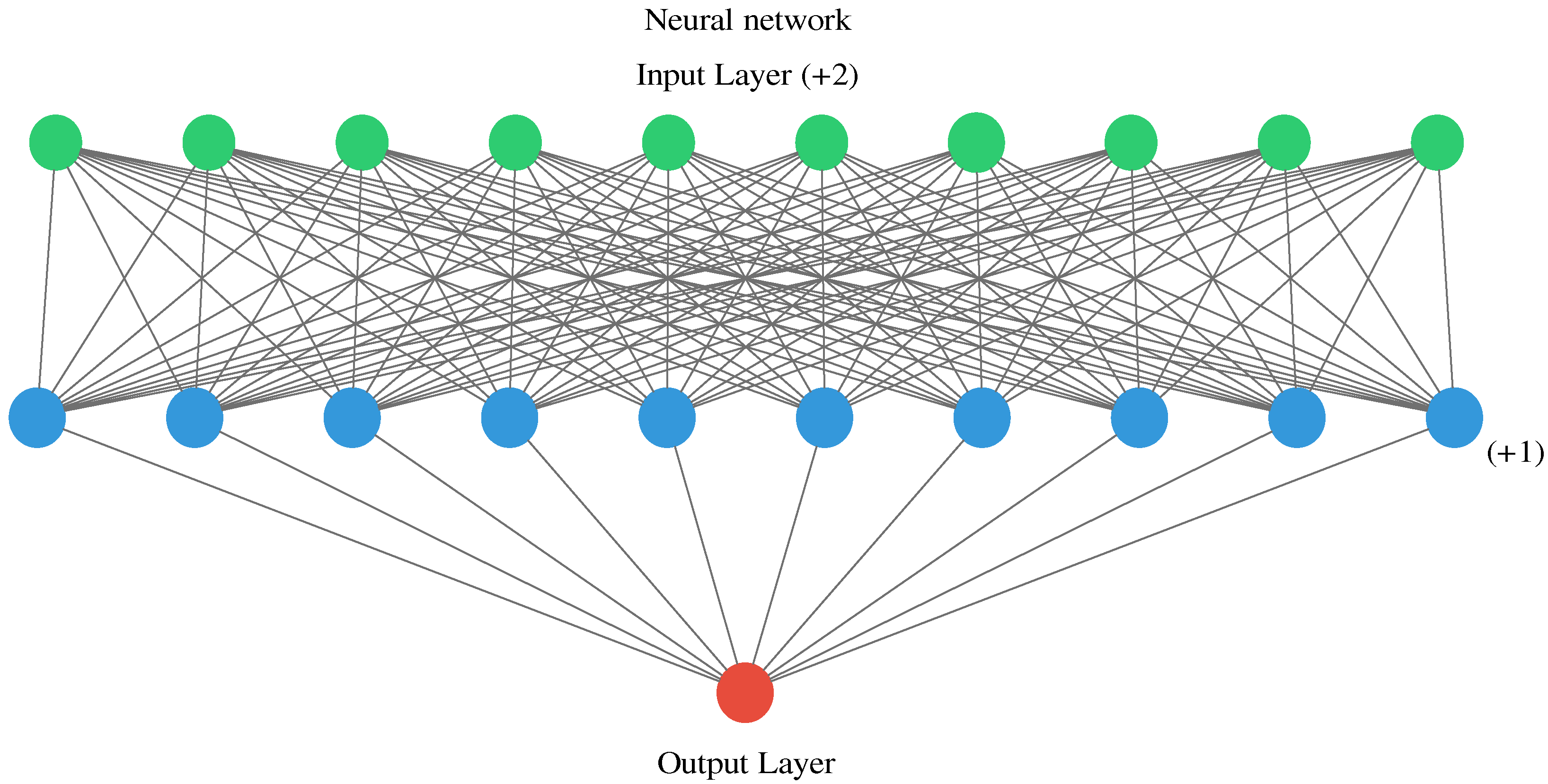
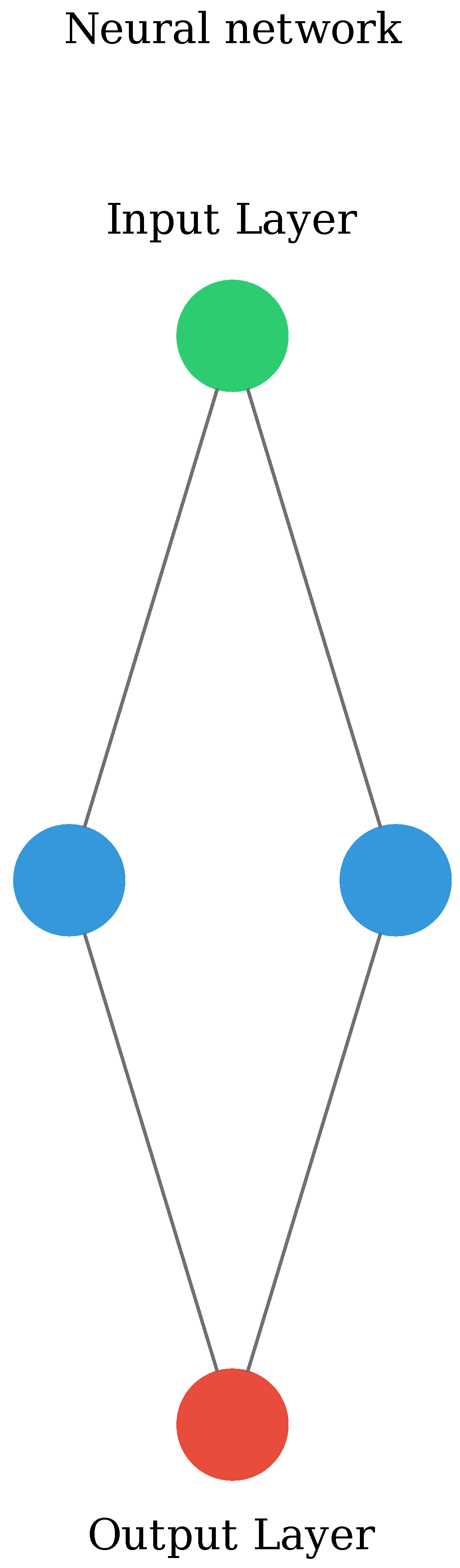
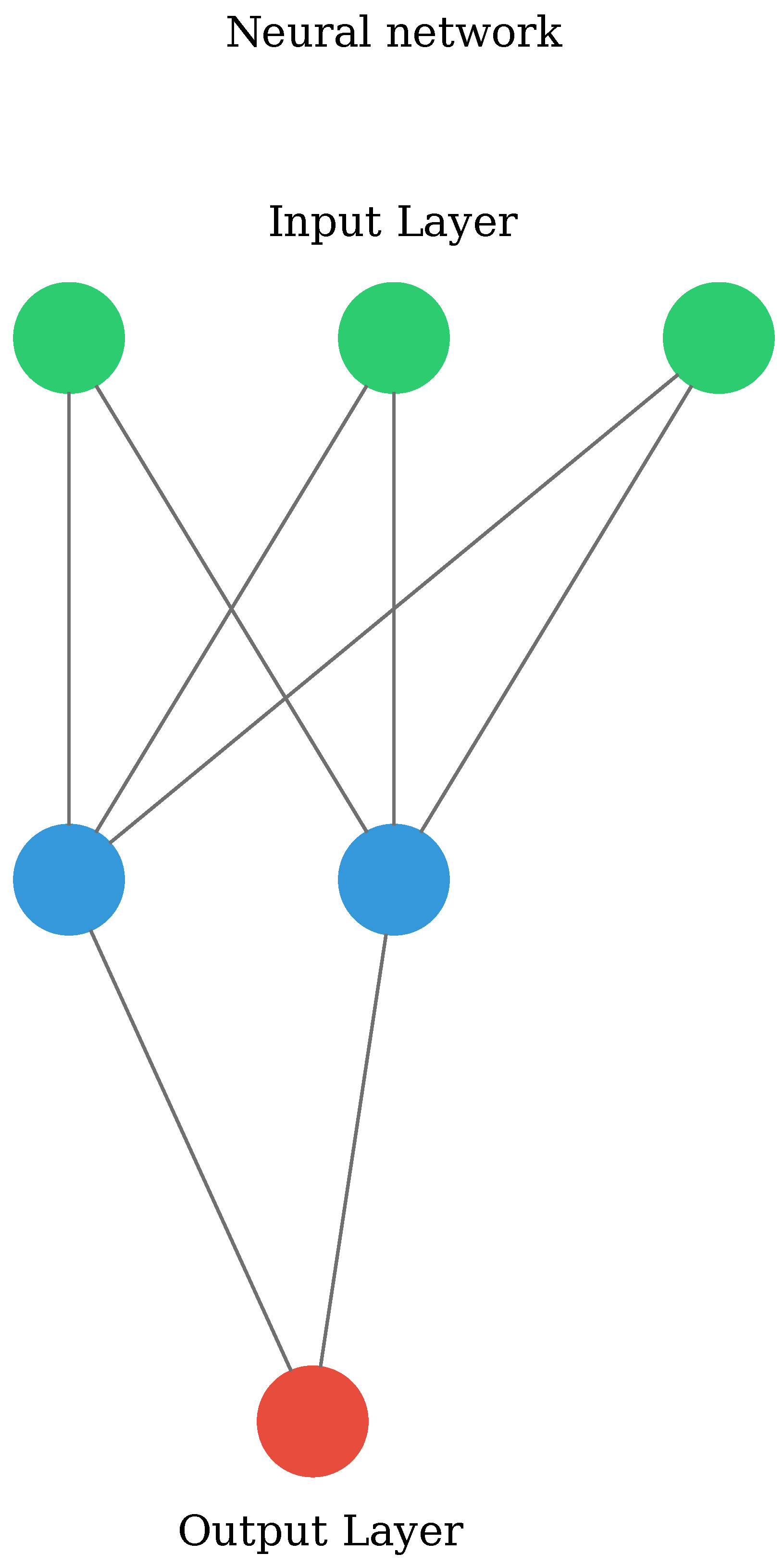
The developed global NN has a relatively simple architecture, shown in Figure 1. It has three layers: an input layer, a hidden layer, and an output layer. In the applicational NN model, the input layer has 12 nodes, the hidden layer has 11 nodes, and the output layer has one node, since the goal of this NN model is to predict the net SW radiative flux at the TOA. It is worth noting that the heuristic NN model developed in Section 3.1 has a simpler configuration (see descriptions there).

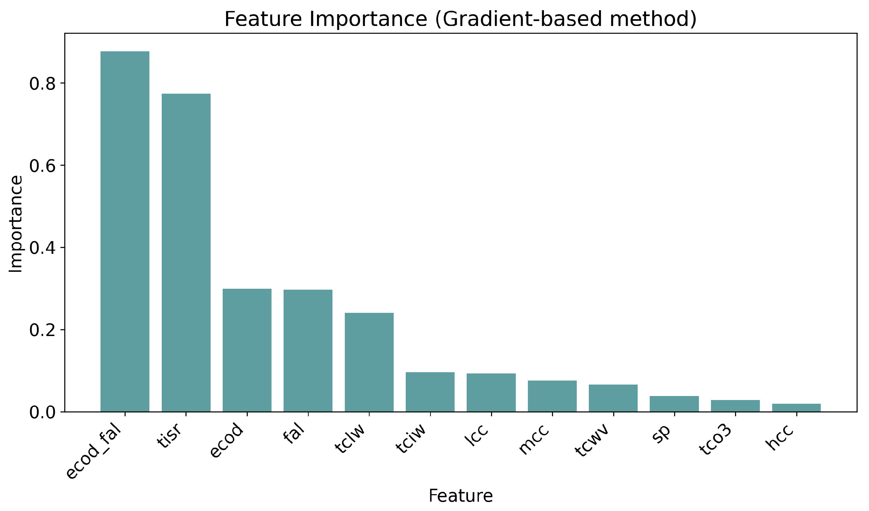
We identified 11 key atmospheric and surface input variables that are important for radiative transfer and that exert a significant influence on radiative flux, these are listed in

Table 1. Input and output variables of the neural network model.

Abbreviation	Description and Units
Input Variables
ECOD	Effective cloud optical depth (Equations (A3) and (A4)), (0,1)
ECOD · FAL	Effective cloud optical depth times forecast albedo, (0,1)
FAL	Forecast albedo, (0,1)
HCC	High-cloud cover, (0,1)
LCC	Low-cloud cover, (0,1)
MCC	Medium-cloud cover, (0,1)
SP	Surface pressure, Pa
TCIW	Total cloud ice water, kg/m2
TCLW	Total cloud liquid water, kg/m2
TCO3	Total column ozone, kg/m2
TCWV	Total column water vapor, kg/m2
TISR	TOA incident solar radiation, W/m2
Output variable
TSR	Total solar radiation, $W/m^2$

, and the feature importance test results are presented in Figure A3. Similar to radiative transfer models (RTMs), only the atmospheric state variables are used to predict the radiative flux, different from the model of Zhu et al. [15] used to demonstrate the NN-based feedback quantification concept. To obviate the necessity for geographic coordinates or temporal information, the NN uses TOA incident solar radiation (TISR) as one of the predictor variables.

All input variables are normalized to the range of $[-1,1]$ using the min–max normalization method, as follows:

$$x_{normalized}=(b-a)\frac{x-min\left(x\right)}{max\left(x\right)-min\left(x\right)}+a$$

(9)

Here, a is the lower range ($a=-1$), b is the upper range ($b=1$), and $min\left(x\right)$ and $max\left(x\right)$ are the minimum and maximum of the input variable x in the training dataset.

The activation function used for the hidden layer is the hyperbolic tangent (tanh). The range of the tanh function is $[-1,1]$. Hence, the output of a tanh function does not have the positive systematic bias found in the output of other activation functions, for example, the logistic function, and it also has the advantage of converging faster [24].

A cost function is used to analyze how well the model fits the data given, which determines a numerical value representing the deviation, or degree of error, between the model representation and the data; the greater the value, the greater the error. The function used is given in Equation (10). The model parameters are initialized randomly and then adjusted using a gradient descent method. The learning rate is set to be 0.001, which determines the convergence speed of the model.

$$\mathrm{MSE}(y,\widehat{y})=\frac{1}{N}\sum _{i=0}^{N-1}{(y_i-{\widehat{y}}_i)}^2$$

(10)

After all model parameters are adjusted in the initial epoch (iteration), the modified model is employed to reevaluate the error. The training process stops when the error falls below a predefined threshold value of 0.0001, or if the number of iterations reaches 900, or if the model’s performance shows no improvement after 10 iterations. At this point, the parameters are fixed as the final NN model parameters. The optimization method employed in this study is the Adam optimizer implemented through the Keras framework.

Zhu et al. [15] developed a set of 12 global NN submodels, each designed for a particular calendar month. In this study, the NN was trained using data from all 12 months of even-numbered years within the time period from 1990 to 2020, encompassing a total of 16 years of training data. Subsequently, the NN’s performance was tested using data from the odd-numbered years within the same period. This approach allows the utilization of a single NN model applicable for all calendar months, facilitating the process of feedback quantification.

3. Results

In this section, we first introduce a heuristic neural network model designed to deepen our understanding of how NNs perform in the evaluation of radiative fluxes. This model also aims to capture the nonlinear relationship between the fluxes and key atmospheric variables, such as surface albedo and cloud cover. While initially trained on simulated flux data, this heuristic NN model serves as the precursor to the full NN trained with reanalysis data and used to quantify feedback.

Then, the performance of the full NN is assessed through a series of tests of different orders. The first test involves examining the NN model’s predictive capabilities with respect to the flux data. Subsequently, we employ established radiative kernels as a benchmark to assess the radiative sensitivity. Finally, an evaluation of the disparities between kernels, arising from their dependence on atmospheric states, is conducted. This comprehensive validation process is crucial in establishing the credibility and applicability of the NN model within the broader context of radiative feedbacks.

3.1. Heuristic Neural Network Model

The Arctic exhibits a pronounced nonlinear radiative feedback, as extensively discussed in prior studies [9,27,28,29]. As highlighted by Huang et al. [9], one of the most noticeable manifestations of this nonlinearity is the surface albedo feedback. First, we examine this nonlinear effect at an arbitrarily selected location in the Arctic (lat = $84°$, lon = $17.5°$).

3.1.1. Univariate Feedback

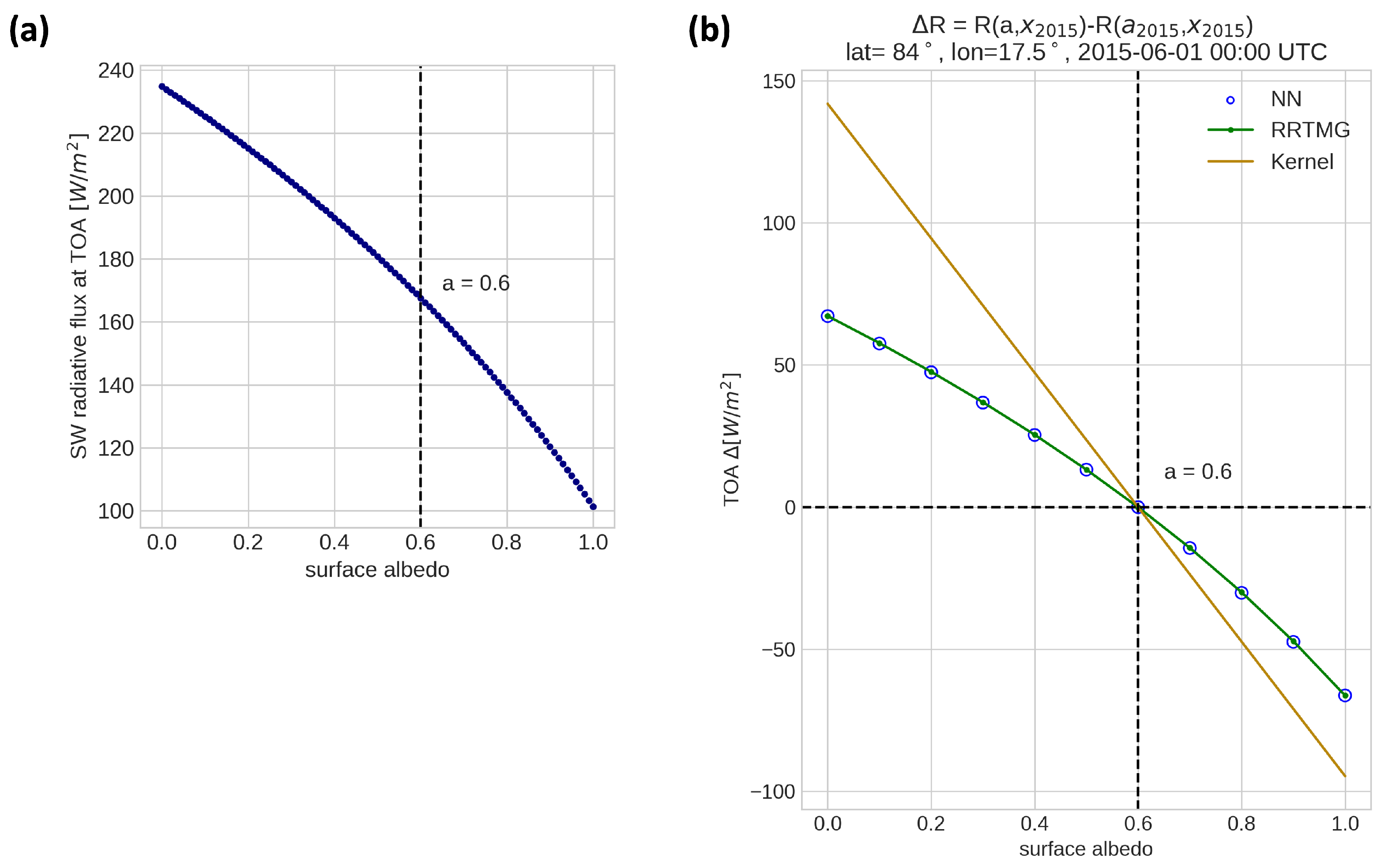
For the atmospheric conditions on 1 June 2015, at the chosen location, we employ the PRP method on the surface albedo variable. We systematically perturb the surface albedo variable from 0.0 to 1.0 in increments of 0.1 in order to obtain the radiative fluxes at the TOA using the Rapid Radiative Transfer Model (RRTMG). These fluxes are used for the training and testing of a NN, which adopts a very simple architecture, featuring only one input variable: surface albedo. Because of its simple architecture, the equation that defines the NN model (Equation (A1)) is also straightforward. This NN model comprises a single hidden layer with two nodes, and one output variable (Please refer to Figure A1). The objective of this NN model is to verify its capability in replicating the intricate nonlinear relation between the flux and surface albedo.

The nonlinear relationship between the shortwave flux and surface albedo is shown in Figure 2a, obtained from the PRP method using RRTMG and from the NN method, respectively. The NN was able to reproduce the nonlinearity for this experiment. In contrast, the kernel method presents a linear relationship between the feedback and the feedback variable, since it is based on linear assumptions. Through this, we confirmed that the NN model can well represent the univariate nonlinearity in the surface albedo feedback.

3.1.2. Bivariate Feedback

Given a bivariate feedback signifies the reciprocal influence of two variables on each other, we extend our perturbation approach to include the cloud cover variable. In systematically exploring the relationship between albedo and cloud cover, we vary the cloud cover values from 0 to 1 in increments of 0.1. This approach aims to offer a comprehensive analysis of the mutual interactions between these variables. Additionally, the configuration of the NN is adapted accordingly (Please refer to Equation (A2) and Figure A2). In this scenario, three input variables are considered: surface albedo (a), cloud cover ($cc$), and their product ($a·cc$). The addition of the product variable enhances the model’s representation of atmospheric absorption and multi-scattering between surface and clouds. A similar consideration was employed in the regression model introduced by Yu and Huang [30] and shown to considerably improve performance. This experiment allows us to examine the bivariate dependence of radiation on surface albedo and cloud cover.

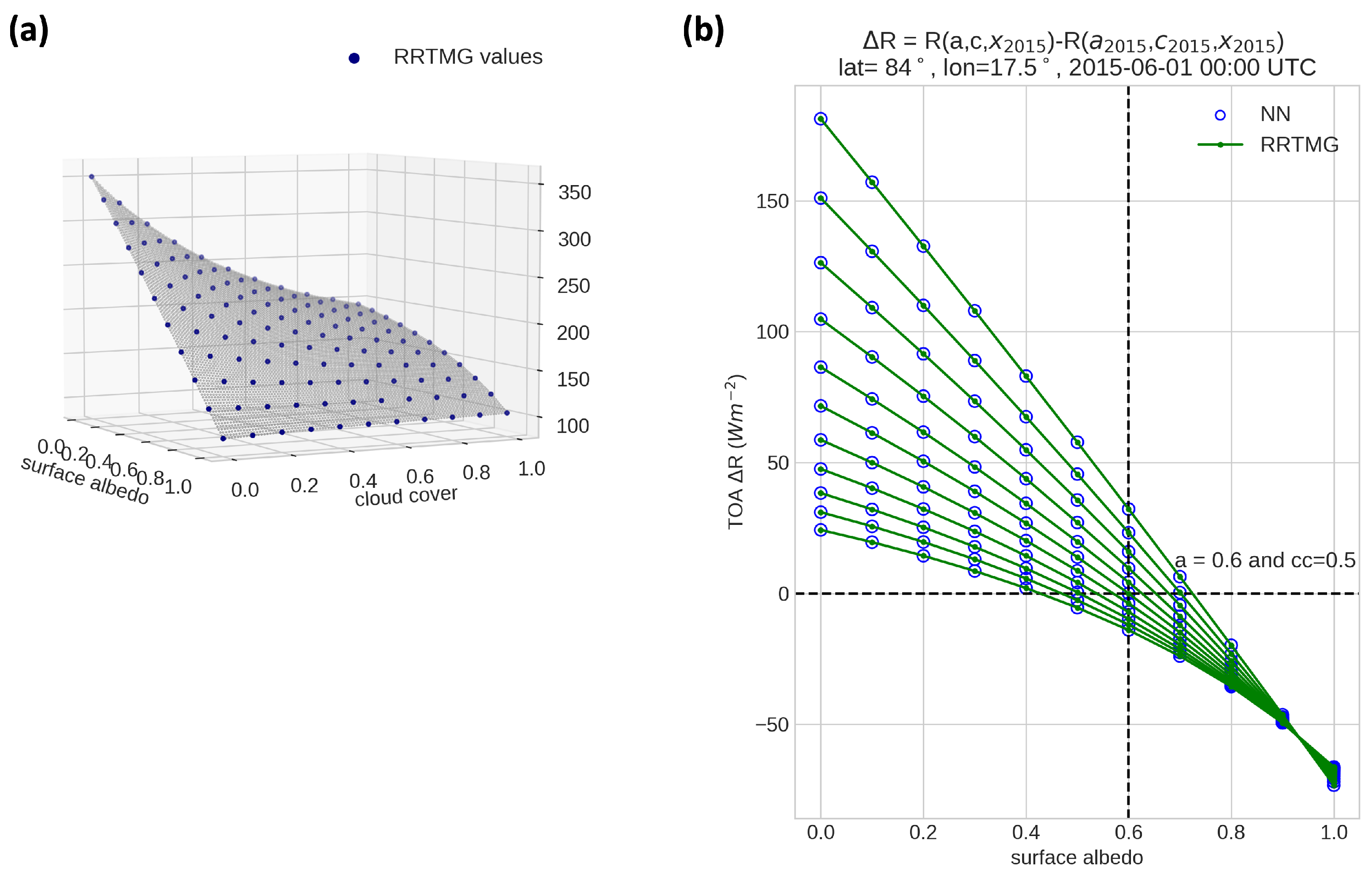
For the bivariate analysis, an interpolation was performed on the flux data, as visualized in Figure 3a, to better perceive the nonlinear relationship between surface albedo, cloud cover, and flux. The resulting bivariate feedback is presented in Figure 3b, revealing a distinct nonlinearity and degeneracy of the feedback values: the same surface albedo perturbation can lead to multiple feedback values when the cloud cover takes different values. This degeneracy is especially pronounced at lower albedo values. Figure 3b shows that the prediction of the NN can well-capture the RRTMG truth of the bivariate dependency of the radiation flux on the two state variables surface albedo and cloud cover.

The results indicate the NN’s effectiveness in capturing the nonlinearity, distinguishing it from linear methods like the kernel approach. The addition of the multiplication of surface albedo with cloud cover improved the performance of the model. The NN predicts the bivariate dependency of the radiation flux on surface albedo and cloud cover, aligning with the results from radiative transfer models.

3.2. Zero-Order Test: Prediction of the NN Model on the Flux Data

The heuristic tests above confirm that NN models can emulate the nonlinear relation between the radiation flux and atmospheric state variables, although the tests were conducted only at an arbitrary location and with idealized state variable perturbations. To further test the ability of the NN model to predict the radiative flux and its variations under realistic conditions, we next train and test a full NN model with global reanalysis data.

The model’s training encompasses the data of all 12 months of even-numbered years within the timeframe from 1990 to 2020. For validation, data from the odd years within the same time period is employed. The NN model’s performance is quantitatively evaluated using the mean bias error (MBE) and root mean square error (RMSE).

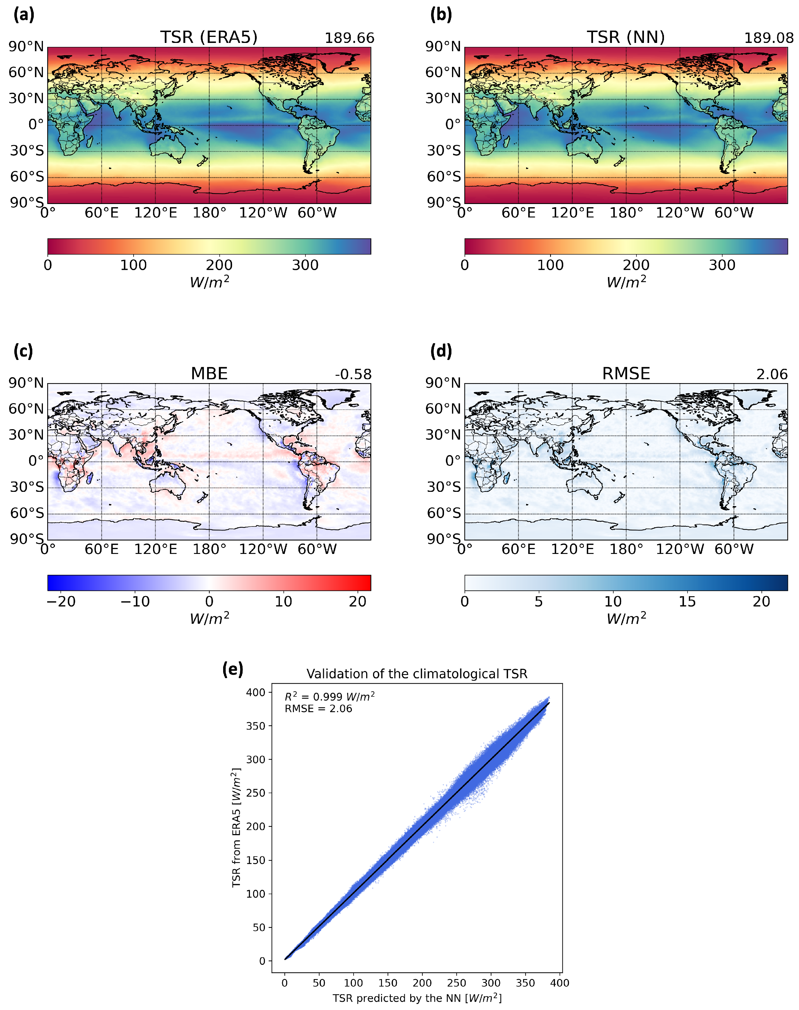
In order to asses the model’s performance, we compare the predicted net shortwave radiative flux at the top of the atmosphere (TOA) against the reanalysis data from ERA5. In Figure 4, it is shown that the model reproduces the radiative flux on a global scale (Figure 4b), although several deficiencies in the prediction are also noticed, including an underestimation of the flux values in the polar regions and relatively worse performance in the regions of elevated topography, such as Greenland and the Andes in South America.

The mean value of the net SW flux at the TOA from ERA5 stands at 189.66 W/m², while the NN’s predictions average 189.08 W/m². For the entire region, the MBE stands at −0.58 W/m², and the RMSE is 2.06 W/m². It is worth noting that inter-RTM biases in their simulated radiative fluxes can be of comparable magnitudes.

Comparison with reanalysis data shows global-scale reproduction of the radiative flux, but with some deficiencies, including underestimation in polar regions and lower performance in elevated-topography areas like Greenland and the Andes. It is noted that biases in simulated radiative fluxes by different models can be comparable in magnitude. A radiative sensitivity test is required to further test the NN model.

3.3. First-Order Test: Radiative Sensitivity

Radiative sensitivity refers to how the radiative flux responds to climate perturbations, which is crucial for quantifying climate feedback and comprehending climate variability. The kernels derived from radiative transfer models have found wide application in evaluating climate forcing and feedbacks. In this study, we take advantage of existing global datasets of surface albedo kernels to test the ability of the NN model to represent the first derivative of the radiative flux.

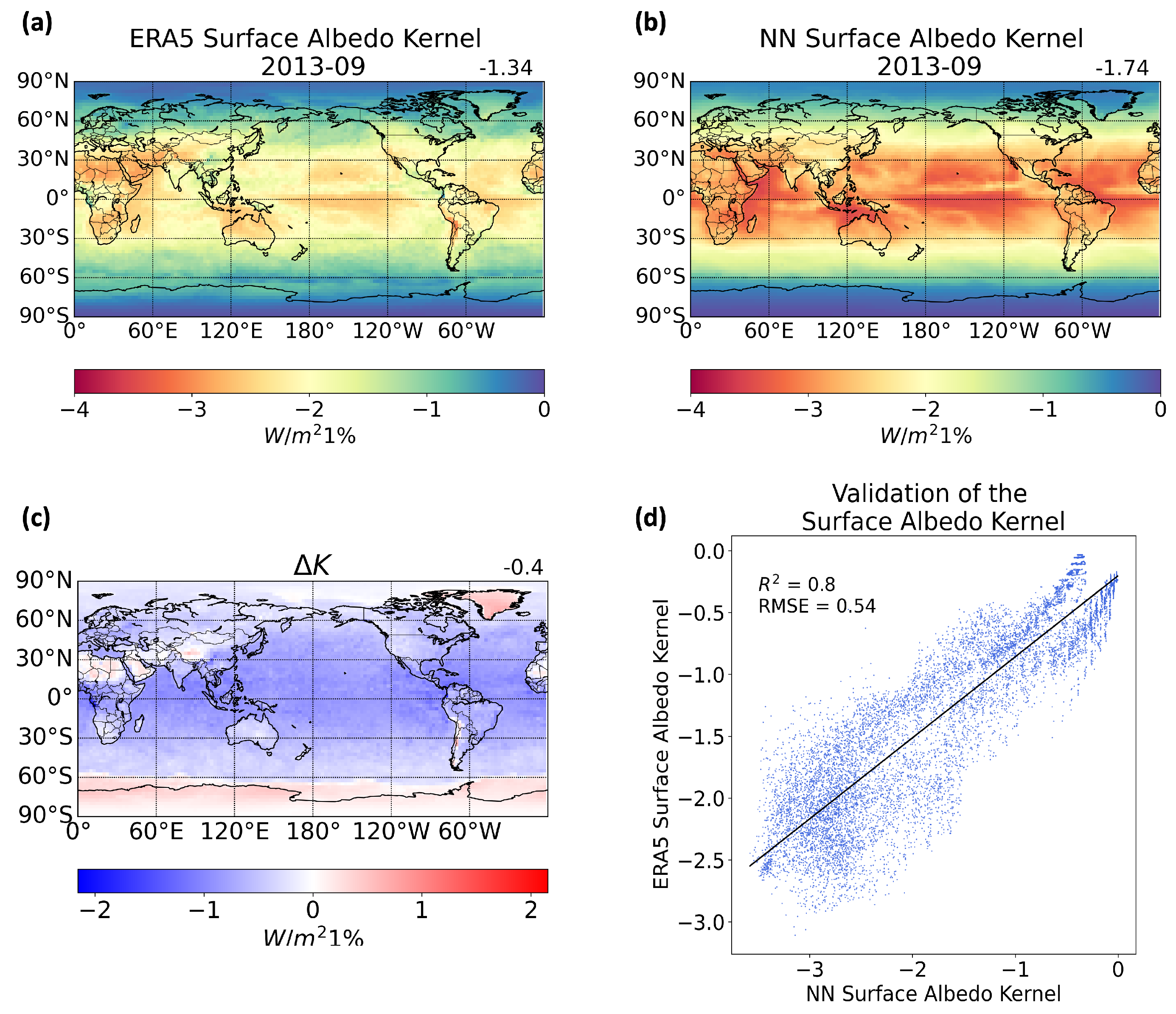
Using the trained NN model, we emulate surface albedo radiative kernels through incremental perturbations of the surface albedo variable at $1\%$. This allows for comparison to kernels computed using an RTM based on ERA5 data, produced by Huang and Huang [22]. After applying a perturbation to the surface albedo for September 2013, we obtain the radiative flux responses as predicted by the NN model. The values for the radiation flux change range from 0 to 3.7 W/m² (Figure 5b).

The magnitude of the radiation change values is as expected. Consider, for example, oceanic regions within the subtropical subsidence area. These regions are characterized by high solar insolation and minimal cloud cover, leading to a maximum radiative sensitivity to surface albedo perturbation. The solar constant is approximately 1360 W/m², rendering a diurnally averaged solar insolation of about 340 W/m². Given the dark ocean surface, a $1\%$ increase in surface albedo implies that $1\%$ of the initial 340 W/m² should be reflected, equating to approximately 3.4 W/m². This aligns well with the values presented in Figure 5b.

In the case of the intertropical convergence zone (ITCZ), the radiative sensitivity values are notably reduced, owing to the persistent and extensive cloud layer. Consequently, altering surface albedo in the presence of such cloud cover exerts minimal influence on the radiation reaching the top of the atmosphere, as the cloud layer effectively masks its effects. Therefore, the observed patterns in the radiative sensitivity values computed with the NN model align with expectations. This suggests that the NN model, at least in a qualitative sense, successfully captures the dependency of the radiative sensitivity on cloud cover. Compared to the radiation change measured by the kernel dataset, it is noticed that the kernels computed using the NN has higher values than the ERA5 kernels. The difference between them is shown in Figure 5c and is represented by Equation (11).

$$\Delta K=K^{ERA5}-K^{NN}$$

(11)

$$=[R^{ERA5}(fa{l}^{2013+1\%},X^{2013})-R^{ERA5}(fa{l}^{2013},X^{2013})]$$

$$-[R^{NN}(fa{l}^{2013+1\%},X^{2013})-R^{NN}(fa{l}^{2013},X^{2013})]$$

In summary, the result here demonstrates how the neural network works in terms of predicting radiative sensitivity. The taining does not explicitly constrain this aspect, it trains the NN to predict radiation values under different atmospheric conditions. But a remarkable performance of the NN model is that it also can tells us about radiative sensitivity, it captures to some extent the radiative transfer principles. It smartly knows that in these cloudy regions the same $1\%$ surface albedo perturbation can lead to less radiation change.

3.4. Second-Order Test: Radiative Sensitivity Difference

Radiative kernels serve as mathematical representations of how various atmospheric properties interact with incoming or outgoing radiation. These interactions are crucial for comprehending climate dynamics. The differences between kernels primarily stem from variations in the physical attributes of the atmosphere under varying conditions. For example, changes in sea ice extent can significantly impact the absorption and reflection of incoming solar radiation, leading to variations in the radiative sensitivity to surface albedo, as illustrated in the heuristic tests above (see Figure 2b).

However, in the meantime, atmospheric conditions co-varying with surface albedo may also affect the radiative sensitivity to the surface albedo. To investigate how such coupled effects jointly determine the surface albedo feedback, we examine the albedo kernel difference between two representative years: 2012, which represents an Arctic sea ice minimum year; and 2013, which is a normal year in terms of sea ice extent.

In September 2012, Arctic sea ice reached its minimum extent recorded by satellite observations since 1979. Conversely, the average sea ice extent for September 2013 was 32% higher compared to September 2012 [31]. Given this significant shift in sea ice extent, as well as other climate state variables such as cloud cover, the surface albedo kernel difference between the two Septembers in 2012 and 2013 renders a second-order test of the NN prediction, i.e., in terms of a second-order derivative of the SW flux prediction.

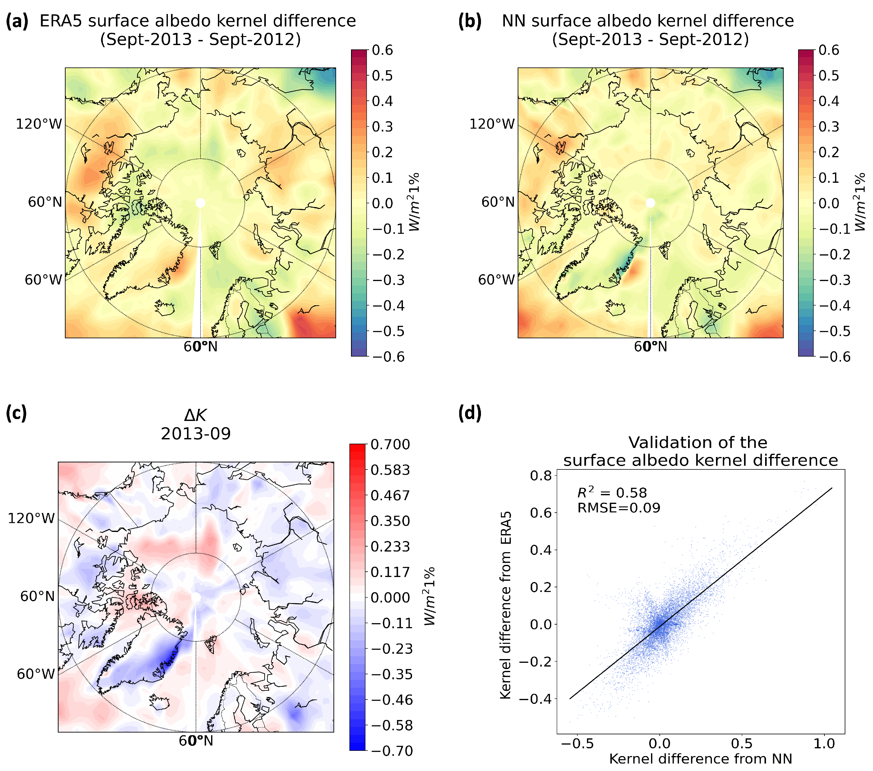
Figure 6 shows that the NN predictions are generally in agreement with the reference kernel values from the ERA5 kernel dataset (as computed by a physical model, Huang and Huang [22]) in terms of the kernel value difference. This demonstrates the NN’s ability of emulating the surface albedo feedback in different climates. However, discrepancies are also noticed.

In 2013, due to a higher sea ice extent, regions like the Canada Basin and the East Siberian Shelf exhibited elevated surface albedo values. Based on the dependency on the albedo value, as illustrated in Figure 2b, we would anticipate larger kernel values (higher sensitivity) in 2013 compared to 2012. This behavior aligns well with the kernels obtained from the ERA5 dataset (Figure 6a). At around 75° latitude from 120° W to 150° E, there are more negative values, indicating higher sensitivity.

However, the NN model (see Figure 6b) shows slightly positive values in this region. This discrepancy can be attributed to the coexistent sensitivity between surface albedo and clouds, which is biased in the NN model. To validate this explanation, we test $\Delta K^{*}$ and $\Delta K^{**}$, as shown in Equations (12) and (13). The year 2012 serves as the baseline year ($K^{2012}$) and the kernel differences ($\Delta K^{*}$) are generated when the sole varying factor between the two NN kernels is the surface albedo difference. This kernel difference (Figure 7b) aligns well with the pattern from the difference of surface albedo between September 2013 and September 2012 (Figure 7a) and also shows the expected negative values, indicating that the trained NN model can emulate well the univariate dependence of albedo feedback on the surface albedo value.

$$\Delta K^{*}=K^{2013*}-K^{2012}$$

(12)

$$=[R(fa{l}^{2013}+1\%,X^{2012})-R(fa{l}^{2013},X^{2012})]-K^{2012}$$

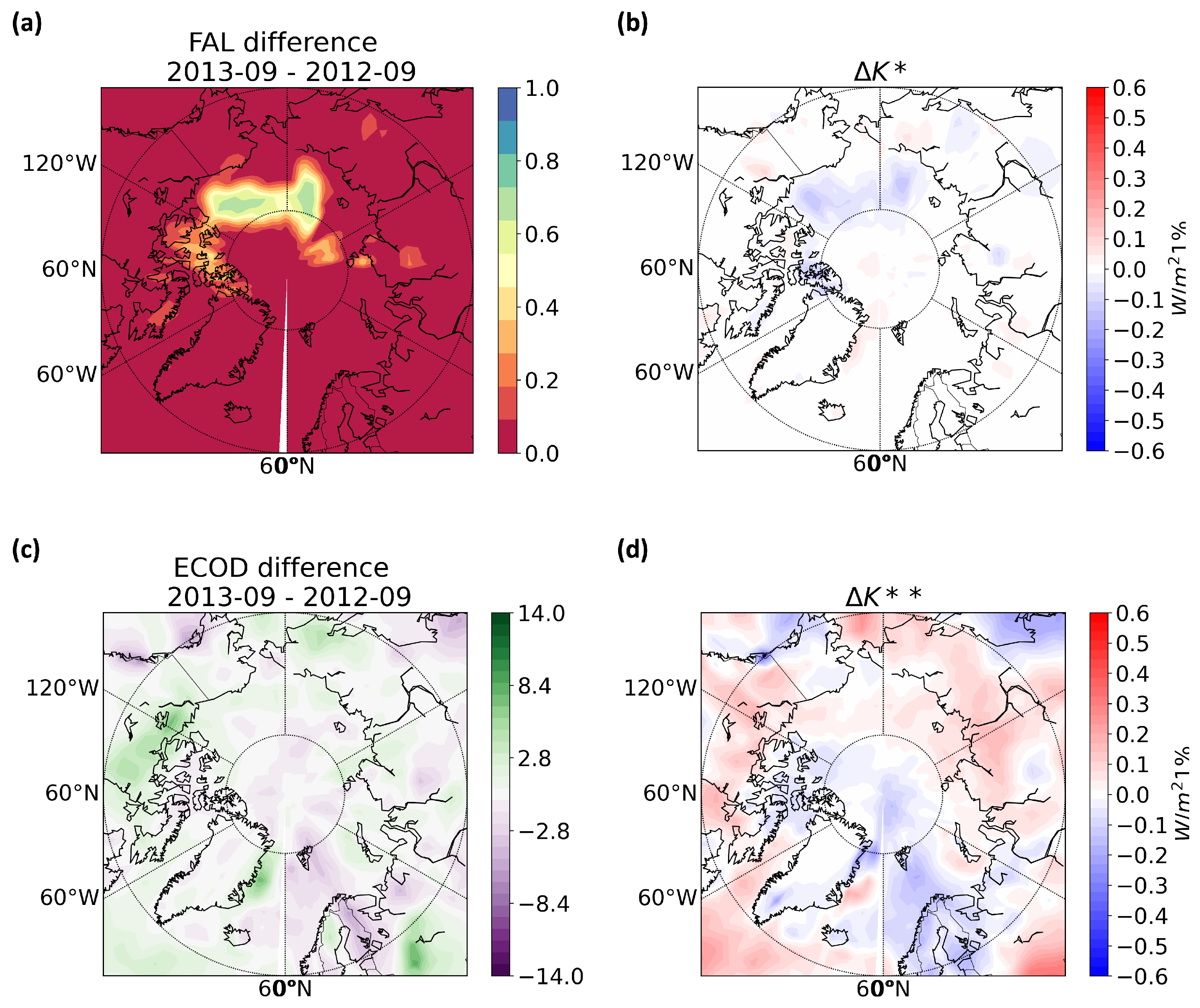
To further verify the cloud (multivariate) impact, the cloud field of 2012 is replaced with the cloud fields (ECOD, HCC, LCC, MCC, TCIW, and TCLW) of 2013 to investigate the kernel difference induced, $\Delta K^{**}$. Figure 7d shows the impact of the cloud field on the kernel value. The Canada Basin and the East Siberian Shelf exhibit positive values, confirming that the positive values in the NN surface albedo kernel difference (Figure 6b) are due to the coexistent sensitivity between surface albedo and the cloud field. We show the effective cloud optical depth (ECOD) variable as a representative variable of the cloud field variables in the NN. Corroborating our explanation, the ECOD difference between September 2013 and September 2012 aligns well with the pattern of $\Delta K^{**}$, as shown in Figure 7c,d. From the resemblance between Figure 7d and Figure 6b, we can also see that the multivariate dependence of the NN model, and particularly the dependence on clouds, seems to dominate the NN-predicted kernel value difference between these two years. We find this to be a major limitation of the NN model trained with the current strategy.

$$\Delta K^{**}=K^{2013**}-K^{2012}$$

(13)

$$=[R(fa{l}^{2012}+1\%,cl{d}^{2013},X^{2012})-R(fa{l}^{2012},cl{d}^{2013},X^{2012})]-K^{2012}$$

In conclusion, we find the NN has hits and misses in emulating the multivariate dependency of the radiative sensitivity (in the case of albedo feedback). When atmospheric conditions co-vary with surface albedo and drive the feedback value to opposite directions, this creates a challenge for the NN model, as the training so far is at the zeroth order and does not directly constrain such higher-order dependence, which can be a primary aim of future investigations.

4. Discussion

The present work introduces a heuristic neural network model aimed at deepening our understanding of how NNs perform in the evaluation of radiative fluxes. This model is designed to capture the intricate, nonlinear relationships between radiative fluxes and key atmospheric variables, such as surface albedo and cloud cover. The initial training on simulated data serves as a foundation towards the development of a more sophisticated NN model utilizing reanalysis data. This progression is pivotal in assessing the model’s applicability and reliability in the context of radiative feedback mechanisms.

The analysis of the heuristic NN model for surface albedo feedback in the Arctic yields noteworthy results. Trained with systematically perturbed surface albedo values, the model successfully replicates the nonlinear relationship between flux and surface albedo. This suggests that the NN model has the capacity to discern atmosphere–surface interactions. Furthermore, the extension to bivariate feedback analysis, incorporating cloud cover as an additional variable, and particularly in the form of the multiplication between surface albedo and cloud cover, enhances the model’s representation of atmospheric absorption and scattering processes.

The introduction of a global NN model trained on reanalysis data from ERA5 represents a significant advancement compared to previous works such as Zhu et al. [15], who used different submodels for different calendar months and included location variables as predictors. The primary advantage of the neural network (NN) approach, in contrast to existing methods, lies in its ability to incorporate nonlinear processes in the evaluation of radiative feedbacks. This aspect is notably absent in conventional linear methods. The model’s ability to reproduce radiative flux on a global scale highlights its effectiveness. However, there is still room for improvement as the performance at the poles as well as in regions of elevated topography is subject to relatively large errors.

We have used global data of multiple years for the training which should have encompassed most possibilities in terms of radiation variability and its relation to geophysical variables. The purpose of the NN model is to represent their relationship as governed by radiative transfer physics, for which we believe the dataset is sufficiently diverse. The generalization to other datasets, e.g., from GCMs, would have to be assessed case by case as it requires bias correction, which is beyond the scope of this study, but we intend to address in future.

The series of tests conducted to assess the performance of the NN model demonstrate the need and advantage of the NN approach. By examining the NN’s predictive capabilities against flux data and comparing it with established radiative kernels, the model demonstrates its potential to capture radiative sensitivity. The comprehensive evaluation of disparities between kernels originating from inherent physical differences in atmospheric states provides valuable insights into the model’s performance.

The assessment of radiative sensitivity captured by the NN model against the ERA5 kernels obtained from a physical (radiative transfer) model reveal that the current training, although not directly constraining the radiative sensitivities at the first or second order, enables the NN model to emulate these sensitivities to some extent. The trained NN model can qualitatively learn both the univariate and multivariate nonlinear dependency of the radiative flux, although quantitatively the learned relationship is subject to biases. This points to the possibility of improvements by reinforcing the sensitivity training, e.g., by using the ERA5 kernel data or changing the NN model to predict flux increments (as opposed to fluxes). These may be investigated in future research.

Exploring the impact of incorporating kernel values into the training process would be valuable, especially in regions with intricate topography and low surface pressure. This alternative method has the potential to unveil previously unforeseen patterns and relationships within the data, enhancing the tool’s robustness and adaptability.

In conclusion, the global NN model represents a promising approach for evaluating radiative fluxes and understanding their intricate relationships with key atmospheric variables. The series of tests conducted to assess the model’s performance highlight its potential in capturing radiative sensitivity and quantifying surface albedo feedback mechanisms.