Article

Intermittency Scaling for Mixing and Dissipation in Rotating Stratified Turbulence at the Edge of Instability

by
Annick Pouquet
1,2,*,†,
Duane Rosenberg
3,†,
Raffaele Marino
4,† and
Pablo Mininni
5,6,†
1
Laboratory for Atmospheric and Space Physics, University of Colorado, Boulder, CO 80309, USA
2
National Center for Atmospheric Research, P.O. Box 3000, Boulder, CO 80307, USA
3
Cooperative Institute for Research in the Atmosphere (CIRA), NOAA/OAR Global Systems Laboratory, Colorado State University, 325 Broadway Boulder, Fort Collins, CO 80305, USA
4
CNRS, École Centrale de Lyon, INSA Lyon, Université Claude Bernard Lyon 1, Laboratoire de Mécanique des Fluides et Acoustique, UMR5509, Université de Lyon, F-69134 Ecully, France
5
Facultad de Ciencias Exactas y Naturales, Departamento de Fisica, Universidad de Buenos Aires, Ciudad Universitaria, Buenos Aires 1428, Argentina
6
Instituto de Fisica Interdisciplinaria y Aplicada (INFINA), CONICET—Universidad de Buenos Aires, Ciudad Universitaria, Buenos Aires 1428, Argentina
*
Author to whom correspondence should be addressed.
These authors contributed equally to this work.
Atmosphere 2023, 14(9), 1375; https://doi.org/10.3390/atmos14091375
Submission received: 9 August 2023 / Revised: 24 August 2023 / Accepted: 26 August 2023 / Published: 31 August 2023

Abstract

:
Many issues pioneered by Jackson Herring deal with how nonlinear interactions shape atmospheric dynamics. In this context, we analyze new direct numerical simulations of rotating stratified flows with a large-scale forcing, which is either random or quasi-geostrophic (QG). Runs were performed at a moderate Reynolds number R e and up to 1646 turn-over times in one case. We found intermittent fluctuations of the vertical velocity w and temperature θ in a narrow domain of parameters as for decaying flows. Preliminary results indicate that parabolic relations between normalized third- and fourth-order moments of the buoyancy flux w θ and of the energy dissipation emerge in this domain, including for passive and active scalars, with or without rotation. These are reminiscent of (but not identical to) previous findings for other variables and systems such as oceanic and atmospheric flows, climate re-analysis data, fusion plasmas, the Solar Wind, or galaxies. For QG forcing, sharp scaling transitions take place once the Ozmidov length scale O z is resolved— O z being the scale after which a turbulent Kolmogorov energy spectrum likely recovers at high R e .

1. Introduction

Much progress has been made in our understanding of turbulence, developing and analyzing experiments, observations, direct numerical simulations (DNSs), as well as numerous theoretical and modeling techniques, among them the direct interaction approximation (DIA) stemming from a renormalization-group (RG) procedure [1], the test-field model (TFM), and related second-order closures, often Markovianized such as the Eddy-Damped Quasi-Normal Markovian (EDQNM), or the quasi-normal scale elimination [2] (see [3,4,5] for recent reviews, and this volume). These flows are complex, due to the large number of eddies interacting non-linearly, as in homogeneous isotropic fully developed turbulence (FDT), and due to their inherent lack of predictability [6,7,8]. Flow structures change in the presence of waves, stemming for example from imposed gravity, rotation, or a strong uniform magnetic field and, specifically, their behaviors differ according to how fast the waves are relative to the eddy turn-over time τ N L = L i n t / U r m s with U r m s , L i n t the r.m.s. velocity and the integral length scale. One of the governing parameters of the resulting dynamics, beyond the Reynolds number, is the ratio G = τ P / τ N L with τ P the characteristic period of the waves; G is the Rossby number in the presence of an imposed rotation, or it is the Froude number in the presence of stratification.
Accurate direct numerical simulations with pseudo-spectral methods were developed in particular at MIT and NCAR in the early 70s and were immediately put to use by Jack Herring to study turbulence, as e.g., in the context of the growth of errors in numerical modeling of the atmosphere [8], of two-dimensional (2D), axisymmetric or QG turbulence [9,10,11], for comparing closures to DNS [12,13], including for non-Gaussian statistics and intermittency in the far dissipation range [14,15]. Jack Herring was central to this introduction of models and DNS to complement experimental and theoretical studies of FDT, and he then moved on to study stratified turbulence [16,17].
Characteristic of turbulence is the presence of localized extreme dissipation in many settings [18,19]. In the ocean, satellite altimetry allows to study the interactions of large-scale planetary or (sub-)synoptic-scale waves with shear structures, as observed for example in the Gulf Stream and the Kuroshio Current [20,21]. Turbulence leads to filamentation, as seen in phytoplankton dynamics forced by hurricanes [22], as well as to energy transfer and dissipative events (e.g., [23,24]). There is also recent radar data indicative of extreme vertical drafts in the (strongly stratified) polar summer mesosphere [25]. Furthermore, waves can change the energy spectra, as demonstrated in weak turbulence [3], detected in the atmosphere [26] and in DNS [27], and as shown in magnetohydrodynamic (MHD) as well [28,29]. Atmospheric data can be related to numerical results for strongly stratified flows showing quantitatively that turbulence interacting with fast waves can be more intermittent than FDT [30,31] in a narrow domain of parameters (see [32] for Solar Wind observations, and [33] for energy dissipation in reconnection events leading also to particle acceleration in the magnetotail).
In this context, we present preliminary results using DNS on relationships between normalized third and fourth order moments taken as proxies to characterize the intermittency and dissipative properties of rotating strongly stratified turbulence, contrasting behaviors for high vs. low kurtosis of the vertical velocity with varying Froude and Reynolds numbers (see next Section for definitions). Similar relationships have been found in the turbulent atmosphere and ocean [34,35,36,37,38], climate data re-analysis and glaciology [39,40], and in fusion plasmas [41,42,43], the magnetosheath, the interplanetary magnetic field or the cosmos [44,45,46,47,48]. Equations, definitions and our numerical methodology are given in the next section. Some of these properties for several field variables for the new runs performed herein are presented in Section 3 for Navier–Stokes and stratified flows. Rotating stratified turbulence is analyzed in somewhat more detail in Section 4. An overview is given in Section 5, and Section 6 presents a discussion and conclusions.

2. Numerical Set-Up

2.1. Equations and Definitions

We perform several sets of numerical simulations for an incompressible ( · u = 0 ) velocity field u = ( u , v , w ) = ( u , w ) with rotation and stratification. The active scalar θ (called in the following temperature) is in velocity units; strictly speaking, θ and the temperature have opposite signs, but they are linearly related through a thermal expansion coefficient. With ν , κ the kinematic viscosity and thermal diffusivity, taken equal, p the pressure, N = [ g z θ ¯ / θ 0 ] 1 / 2 the Brunt-Väisälä frequency, and f 0 = 2 Ω , Ω = Ω z an imposed rotation in the vertical direction of unit vector z , the Boussinesq equations are:
t u + ( u · ) u = p N θ z + 2 u × Ω + ν 2 u + F u ,
t θ + ( u · ) θ = N w + κ 2 θ + F θ .
Two types of forcing for F u , F θ have been implemented, both set in the large scales at a wavenumber k F 2.5 . The first one has random phases and is white noise in time. The second forcing, for the rotating stratified turbulence (RST) case, ensures a quasi-geostrophic balance at all times in the forcing modes (see [11]), following the procedure described in detail in [49] for QG initial conditions with zero vertical velocity. Pressure balance with the Coriolis force in the horizontal is enforced, as well as hydrostatic momentum balance due to gravity (see [50] for a different implementation in a study of balanced dynamics). One might note that the time-scale associated with the forcing, in particular in the case of white noise, may matter in the interactions between waves and eddies, with more waves for short correlation times, in particular at low Froude number for which N becomes comparable to 1 / Δ t , where Δ t is the time-step [27]. The buoyancy flux B f , the kinetic energy dissipation ϵ d u and the potential vorticity P V (point-wise invariant in the absence of dissipation) are:
B f = N w θ ; ϵ d u = ν | ω | 2 ; P V = f z θ N ω z + ω · θ ,
with ω = × u the vorticity. B f is an energy exchange term with the same physical dimension as ϵ d u . It leads to local changes in density in the presence of gravity waves which need to be modeled in large-eddy simulations. Characteristic scales can be defined as the Taylor micro-scale λ T that factors in the dissipation in the inertial range, the dissipation scale η K based on a Kolmogorov spectrum, the buoyancy scale L B measuring the effect of stratification in the large scales, and the Ozmidov scale O z :
λ T = u 2 ω 2 1 / 2 , η K = ϵ d u ν 3 1 / 4 , L B = U r m s N , O z = ϵ d u N 3 1 / 2 ; O z η K = L B λ T 3 / 2 .
The last expression indicates the multi-scale link in the dynamics of the flow between the development of turbulence and its stratification. The dimensionless parameters governing the fluid behavior are the Reynolds, Rossby and Froude numbers, R e , R o , F r , with the Prandtl number P r ν / κ = 1 here:
R e = U r m s L i n t ν , R o = U r m s f L i n t , F r = U r m s N L i n t ; R λ = U r m s λ T ν , R B = R e F r 2 ,
with R λ , R B the Taylor and buoyancy Reynolds numbers. For the purely stratified runs, the forcing scale L f = 2 π / k F is used in the evaluation of the parameters instead of the integral scale L i n t . One also defines the interaction parameter R I B and, when involving gravity through N, the Richardson number R i based on an overall vertical gradient of u , as well as a local gradient Richardson number R i g :
R I B = ω r m s 2 N 2 = ϵ d u ν N 2 = L B λ T 2 ; R i = N 2 z u 2 , R i g = N ( N z θ ) [ ( z u ) 2 + ( z v ] 2 ] , I R i = R i g .
The phenomenological evaluation of kinetic energy dissipation, ϵ D = U r m s 3 / L i n t , is based on expressing that it occurs in an eddy turn-over time, irrespective of the (small) viscosity. When ϵ d u becomes comparable to ϵ D , as in FDT, one has R B = R I B . Note also that R i , R i g , in the absence of uniform shear, are based on large-scale shear resulting from the overall nonlinear dynamics. One can also define a Taylor Froude number F λ and relate it to the other parameters. After simple manipulations, one has:
F λ U r m s N λ T = L B λ T = R e F r R λ = R I B 1 / 2 = O z η K 2 / 3 .
The RST runs cover the three regimes identified in [51]: wave and viscous-dominated at small [ F r , R B ] , eddy-wave interactions at intermediate values, and the eddy-dominated regime with a resolved turbulent inertial range beyond the Ozmidov scale ( O z > η K ). These three regimes can likely be related to the classification proposed in [52] for the nocturnal planetary boundary layer (PBL) into weakly stable, transitional, and very stable regimes: when increasing the Froude number, there is a drop in the Richardson number, particularly marked in the transition regime, and a sharp increase in eddy diffusivities. Another classification of stratified flows can be found in [53] (see also [54,55]) in which the role of viscous dissipation, governed by a small Reynolds number, is particularly emphasized. This is in contrast to the role of fast waves compared to nonlinear eddies, as governed by a small Froude number; the competition between these two effects can be encompassed in the parameter R B = R e F r 2 , or in R I B , but not necessarily uniquely [56]. At low R B , anisotropy comes strongly into play. Previous studies (see e.g., [57]) have shown that when the system is forced three-dimensionally, this results in a significant excitation of wave modes which, as a result of viscous effects, can excite less vortical modes. However, their interactions with waves are still present [58], and we call this regime wave dominated since no turbulence range is excited. We also note that, at a given (high) buoyancy Reynolds number, all three regimes can be identified in the energy spectra in a given flow, provided L B , O z and η K are resolved (see [59] for an analysis of these regimes using a turbulence closure). Different values for R I B can be found when using the energy injection rate F u · u instead of ϵ d u , the two equilibrating only on average. This is particularly relevant when there are strong intermittent fluctuations in the system [60,61], and this balance can also be broken in the presence of an inverse energy cascade. Finally, the skewness and excess kurtosis of a random variable V, with averages taken over three-dimensional (3D) space and with S V G = 0 , K V G = 0 for a Gaussian, are defined as usual, with the following parabolic relation to be tested in this paper, e.g., for V = B f :
S V = V 3 / V 2 3 / 2 , K V = V 4 / V 2 2 3 ; K V ( S V ) = a V S V 2 + b V .

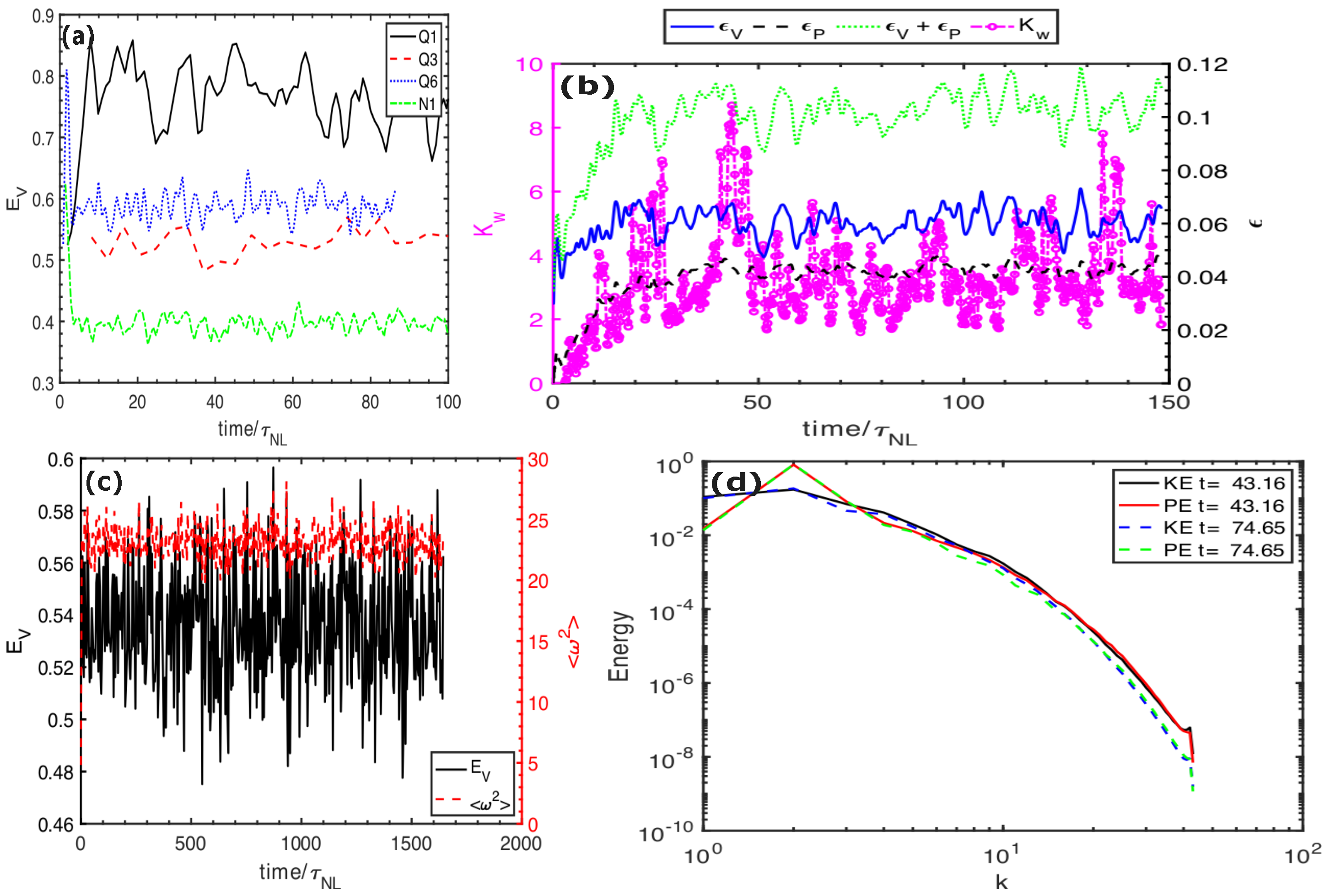
2.2. Overview of the Direct Numerical Simulations

We use a variety of DNS (see Table 1). The runs labeled H are for the hydrodynamic case (Navier–Stokes, N 0 , Ω 0 ); the S i = 1 , 6 runs deal with the Boussinesq equations with Ω 0 . The R , Q runs are RST with random or QG forcing; all these runs have N / f 0 5 , leading to 0.28 R o 3.7 . Smaller Rossby numbers would imply the development of a strong inverse energy cascade (see e.g., [62] and references therein), a cascade that would be altered by the large-scale forcing when there is insufficient scale separation as here. The dependence of kurtosis on skewness for various fields in the presence of both inverse and direct energy cascades is left for future work.
The linear dimension of the cubic grid is n p , varying from 128 to 512. The code is a versatile pseudo-spectral formulation of the time-integration of a large set of partial differential equations for fluid and plasma turbulence, with efficient hybrid parallelism implemented in a periodic box [63]. There is a version of the code in non-cubic geometry, as well as with non-periodic boundary conditions in one direction for the incompressible case [64]. T M is the extension in terms of turn-over time τ N L of the segment of the simulation used to build the statistics, with 41 T M 1646 across all runs. Data is gathered roughly four times every τ N L , but for purely stratified runs, statistics of the dimensionless parameters are taken around the first peak of dissipation in order to avoid the effect of energy accumulation in the slow-mode leading to vertically sheared horizontal winds [65,66]. An estimate of the error on the skewness, and thus of its departure from Gaussianity, is 6 / N S , and twice that for the kurtosis [38,67], N S being the number of independent samples. For our runs, the worst-case gives S > 0.38 for a flow to be determined to be non-Gaussian, and ≈0.06 in the best case. All Taylor Reynolds numbers are above ≈27 and should thus suffice to determine small-scale intermittent properties of the flow [68,69] when properly averaged over long times. In fact, local quasi-singular behavior in the intensity and curvature (morphology) of the vorticity and strain tensor can already be discerned at moderate R λ when accurately evaluating the geometrical properties and anisotropy of the flow close to such structures through a so-called sparseness scale [70,71,72].
Finally, in Table 1, K w M is the maximum over time of the kurtosis of the vertical velocity, a signature of large-scale intermittency and strong dissipation in the transitional regime [30,31,73,74]. Most of the RST runs are at low to intermediate R B with high K w M , as for the stratified runs. How well the runs are resolved is measured through R e s N = k m a x η K , with k m a x = n p / 3 using a standard dealiasing method. R e s N 1 implies that the dissipation scale is resolved by the numerical grid; a , b are the parameters when performing a S 2 + b fits analyzing K ( S ) for the buoyancy flux; r.m.s. errors are between 1.8 and 6.3% for all runs for a, and between 0.8 and 2.3% for b, with respective averages for the eight QG runs of 4.27% and 1.44%. The extent of the turbulent range beyond the Ozmidov scale is R e s T = O z / η K = F λ 3 / 2 ; when greater than unity, a sharp transition occurs in the K ( S ) scaling parameters for both B f and the kinetic energy dissipation ϵ d u (see Section 4 below).
Many studies of stratified flows have been performed [27,53,54,75,76,77,78,79,80]. Small-scale intermittency is present once O z / η K > 1 , whereas at large-scale it is observed in a restricted range of values of R i g strongly peaked for shear instabilities (as well as in a narrow range of F r , R B , R e s T ), without rotation [30], or with it as shown in this paper. An increase in the amplitude of nonlinear P V when going to higher buoyancy Reynolds number is also observed [74,75]. Note also that, in the presence of a strong Coriolis force, a quasi-geostrophic balance is obtained that can lead not only to an inverse energy cascade to large scales (Ref. [62] and references therein), but in fact to a dual constant-flux energy cascade to both large and small scales [81,82,83].

3. Large-Scale and Small-Scale Intermittency in Turbulence

Intermittency, measured by non-Gaussian statistics [14], can modify passive scalar advection such as pollutants, and thus the chemistry within turbulent flows, e.g., through segregation as in the convective boundary layer, in particular when strong shear is present [84] (see [48,85] in the interstellar medium and galactic contexts). These baroclinic instabilities can be abrupt and result in turbulent bursts, reminiscent of large-scale on-off intermittency (LSI). There are in fact several such findings of LSI, starting with the probability distribution function (PDF) of the temperature which can be non-Gaussian (e.g., Métais and Herring [16], Rorai et al. [73]). One of the striking new results in [31] is that dissipation can be stronger locally than for FDT, as quantified by measuring the minimum flow volume needed to reach some level of energy dissipation, say 50%. Close to the peak of intermittency of w , θ , this volume can be as small as 12%, compared to 15% for FDT at a similar Reynolds number, and less than 4% for the active scalar, possibly indicating than a log-normal distribution is not adequate for the statistics of these flows [86] (see [87] for the FDT case). The waves can enhance dissipation in hot spots even when, globally, the flow is constrained by the large-scale, smooth dynamics. Extreme events are observed frequently in the atmosphere, e.g., in terms of w , θ [88], of the rate of energy dissipation [89] as well as for extreme precipitation [90,91]. A possible role in the formation of such structures is through the precession resonance of Rossby waves which was analyzed e.g., in [92,93], leading to their breaking as well as to their interactions with potential vorticity [94,95]. Similarly, in the ocean, wave breaking leads to efficient mixing processes [77,78,79], and observations of double-signed skewness can be the signature of a front, modeled in a dichotomic way for relative vorticity [67] as for the Agulhas current.
A simple non-Gaussian model is to express the PDF for field V as the sum of a normal distribution and its square, the relative weight of the two being governed by an open parameter. When the quadratic term dominates, one finds K V = 3 S V 2 / 2 + b [96]. In fusion plasmas, similar relationships are obtained [41,42,97,98], with different quadratic laws followed by different experiments [43]. The properties of the high-variability parts of turbulent flows, such as shear layers and their relaxation, seem universal and can be described by the model in [34], such shear layers developing at the boundaries [97], or as internal structures due to the turbulence. In fact, high kurtosis for the velocity and temperature at the edge of a shear layer have been found in a DNS of a Kelvin-Helmholtz instability [99], and singular shear layers can lead to intrinsic stochasticity [100]. Moreover, interactions with large scales in fluid turbulence represent roughly 20% of the kinetic energy flux at moderate R e . For structure functions beyond the energy level, including in the absence of waves, the nonlinear interactions are found to be mostly non-local, involving the integral scale [101], but with a tendency towards locality as R e . Large-scale extreme events can arise as well in climatological studies, for example from quasi-resonant amplifications of planetary waves [92]. One also recovers a quadratic K ( S ) law by adding three Gaussian PDFs, a model suitable for climate temperature variability [102], with the result that knowledge of skewness becomes a predictor of kurtosis. In fact, ( S , K ) mapping can be taken as an indicator of the turbulent dynamics in all these flows [44,46,67,96].

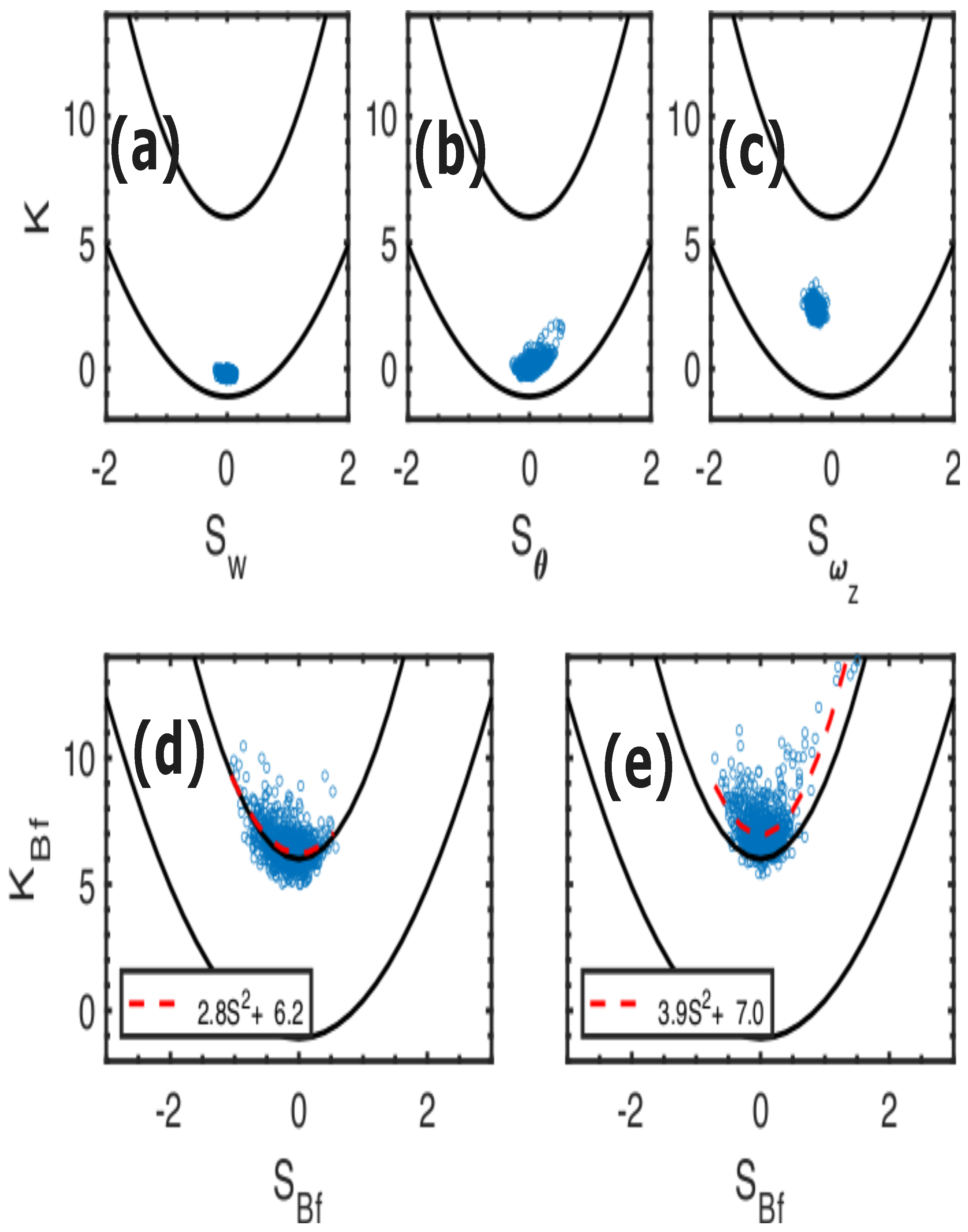
3.1. Is There a Skewness–Kurtosis Relationship for Fluid Turbulence with a Passive Scalar?
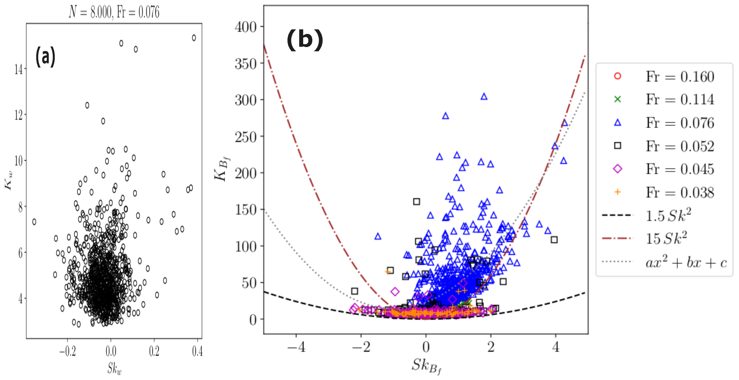
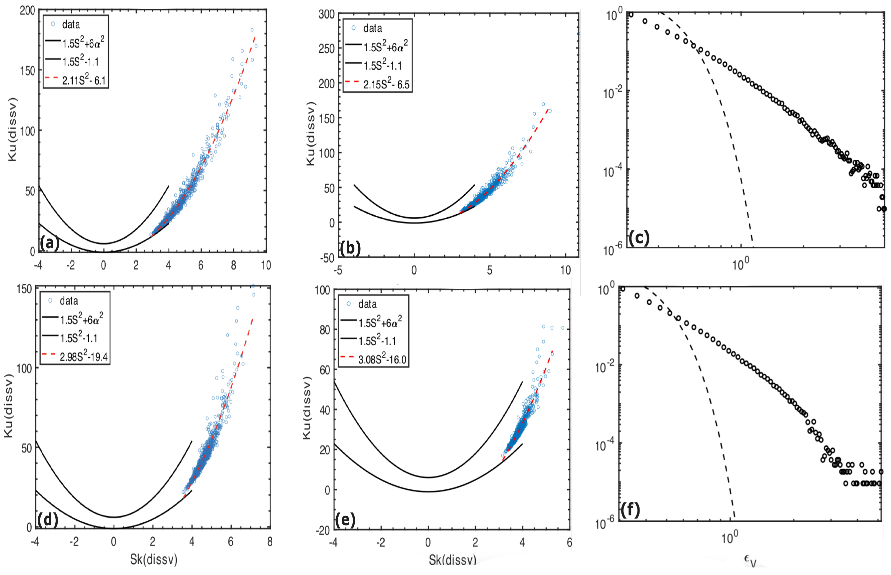
Curiously perhaps, FDT (with a passive scalar) has barely been analyzed in the context of K ( S ) laws. This problem was studied in Herring and Kerr [12] in the decaying context and for P r = 0.5 . The skewness of the velocity was compared with experiments and with predictions of turbulence closures at R λ comparable to what we compute in this paper, but here in the forced case. The flatness evaluated from the DNS was also contrasted with that given by closures (DIA and TFM). Good agreement was observed up to R λ 30 . At high R λ (above 800 or so), the experimental and numerical data reviewed in [103] for fluid turbulence does lend some credence to a relationship K S j , j 2.5 for the velocity derivative, as noted in [43] (see also [104], Figure A6, for a recent estimate of K , S for numerical and experimental fluid turbulence with R λ in excess of 6000). Furthermore, a statistical study of passive scalars in the atmosphere under many physical conditions gives a parabolic relationship, with in some cases rather high values of both S P and K P [36,37]. Several PDFs have been invoked to justify a quadratic relationship between K and skewness S, depending on the tails of such distributions [105], and exponential wings in PDFs of the horizontal vorticity for RST flows have been found [74]. Thus, we briefly discuss first the kurtosis and skewness data for FDT and a passive scalar with P r = 1 .
Figure 1 (top) displays K ( S ) for run H2 for the vertical velocity, temperature and ω z (a–c). At the bottom, K ( S ) is shown for the buoyancy flux B f (we are not considering here the joint w , θ distribution), for runs H1 (d) and H2 (e), with least-square fits for [ a , b ] given in Table 1. Note that, for a unimodal and symmetric distribution, one can derive estimates that improve on the Cauchy-Schwarz inequality, namely K S 2 6 / 5 [106], thus limiting potential closures [107]. In all the K ( S ) figures, two parabolae are drawn, K ( S ) = 1.5 S 2 1.1 and K ( S ) = 3 ( S 2 + 2 ) (using n = 5 in [108], Equation (9b)). The first formulation appears in a variety of data, as described earlier. It should also be mentioned that it is quite close to the approximation developed in [109] (who also considers joint distributions), namely K 16 S 2 / 9 , emanating from an expansion of a PDF assumed to be quasi-Gaussian and first analyzed on data of coastal waves [110] (see e.g., [111] in the context of the Weibull distribution for a model of sea surface wind velocity, and [112] for recent data analysis of strong waves on a beach with a sloping bottom). The second K ( S ) formulation arises from the analysis of stochastically-generated skewed distributions (SGS) for which general K ( S ) relations are obtained. These SGS distributions can be related to Markov processes, thereby shedding some light on the underlying stochastic systems [108]. As expected, no measurable intermittency is seen in Figure 1 in the large-scale field w, with both S and K close to zero, but θ , ω z display measurable non-zero values that are at times higher than those given in Herring and Kerr [12], the forcing likely allowing for wider excursions. In plasmas, the K S 2 law obtains for both quiet and active regions and, in that sense, the relationship itself may not be related to the development of strong turbulence, but rather to intrinsic multi-scale properties of the fields themselves [41]; ϵ d u (not shown) is also close to a quadratic law, but with higher coefficients. Taking ω z as a (skewed) velocity gradient, the values of S , K are in fact consistent with data in [113], but higher Reynolds numbers will have to be explored to see whether a parabolic law actually appears.
Many models describe the interactions between widely separated scales from energy-containing to dissipative eddies. The combination of (weak) fast additive noise and large-scale multiplicative noise is known to produce PDFs with power-law tails [114]. Further examples are on-off intermittency in FDT close to instability [115], the scale-dependent creation of intermittency [116], or the magnetic dynamo problem [117]. Chaotic dynamics can also be seen as quasi-linear behavior forced by non-Gaussian processes whose events in the tail can trigger bifurcations in the system [118]. In this context, let us mention the climate model of Hasselmann [119] which begins with a linear stochastic (Langevin) equation for the temperature anomaly Θ , namely t Θ = λ Θ + η ; here, λ represents the heat flux and η is a noise term modeling small-scale fast fluctuations. One can in fact write λ = λ ¯ + λ with λ ¯ an average, making the noise multiplicative [38] (see [120] for a recent review). Indeed, small-scale eddies are in large numbers, have low energy compared to that of the large scales and are intermittent, leading to complex behavior. This makes it plausible to model them through a stochastic linear noise acting on the slower large scale eddies (see also [121] for another Langevin approach, and [122] for stochastic turbulence models). One can then derive the parabolic relationship in Equation (8) with the expectation that a 3 / 2 , b 0 [38], a finding corroborated by several analyses of climate data. The long-term (monthly onward) climate statistics are Gaussian, but the daily averages reflect the stochasticity of small-scale eddies [38] which also interact with waves. Therefore, on some intermediate temporal scale for the large structures, these small eddies can be viewed as noise, although there exist nonlocal (in scale) interactions between small and large scales. This leads to enhanced dissipation at the level that is needed in order that, in its adimensionalized form and at least in the absence of waves, it be of order unity, both for fluid turbulence [19,123] and for fusion and space plasmas [124,125].

3.2. K ( S ) Relationships for the Buoyancy Flux in the Purely Stratified Case

For strong stratification, the vertical velocity intermittency can be significant, like in the nocturnal PBL [18,34,52], or for DNS in a narrow range of Froude number [30]. Does a K ( S ) relationship ensue in that regime? To answer this question, we examine the results of a series of purely stratified runs with 0.032 F r 0.145 , and with high R e 3000 . At left in Figure 2 is K ( S ) for w for the run with the highest kurtosis of w [30,31]. We observe that there is a large number of data points with large excess kurtosis, but the skewness of w remains close to zero. On the other hand, such is not the case for the buoyancy flux B f shown at right in Figure 2 for all the S runs. In the inset, three parabolae are given (dash; dots; and dash-dots) corresponding to different [a,b] fits. The first remark is that, for stratified turbulence, a parabolic K ( S ) law seems to emerge as well for B f (and for ϵ d u , not shown). Note that practically all runs lie on the lower parabola marked with dash, and showing as an orange cloud of points in the plot. Superimposed on this, for two runs close to the maximum of K w , there is an explosion in the values taken by the kurtosis (blue triangles and black squares, runs S3 and S4). This confirms the analysis performed in [31] that dissipation in this F r range takes high local values; it corresponds to a transitional phenomenon with high intermittency of vertical velocity, flux and dissipation itself, and thus leading to enhanced mixing as we move from regime I (wave dominated) to regime II (eddy-wave interactions), likely similar to what happens in the nocturnal PBL [52]. The a coefficient in front of the quadratic term in the K ( S ) law for the vertical velocity in the PBL is thought to depend on the stability of the layer through R i g [54,126]. Indeed, strong vertical drafts are clearly correlated with R i g 1 / 4 (see [30], Figure 3). It may be that K ( S ) laws are emerging here from the flow being at the edge of instability [127,128]. An analysis similar to that of Vieillefosse [129] yields nontrivial relations between high-order moments of the field gradients near the onset of convective instabilities [130]. An inverse scaling, on more than two orders of magnitude, between two a-priori unrelated parameters, namely one governing stratification (the gradient Richardson number) and one governing the turbulence in the presence of stratification (the buoyancy Reynolds number)– was observed in DNS of rotating stratified flows [51]. One could thus infer that the a parameter just mentioned would depend in a similar fashion on R B . This inverse R i g R B 1 relationship is significant because it implies a strong dynamical effect of vertical shear, and a balance between vertical gradients (of the turbulent horizontal velocity field) and the turbulent isotropic eddies beyond the Ozmidov scale [51], as hinted in fact by several authors over the years in varied contexts.

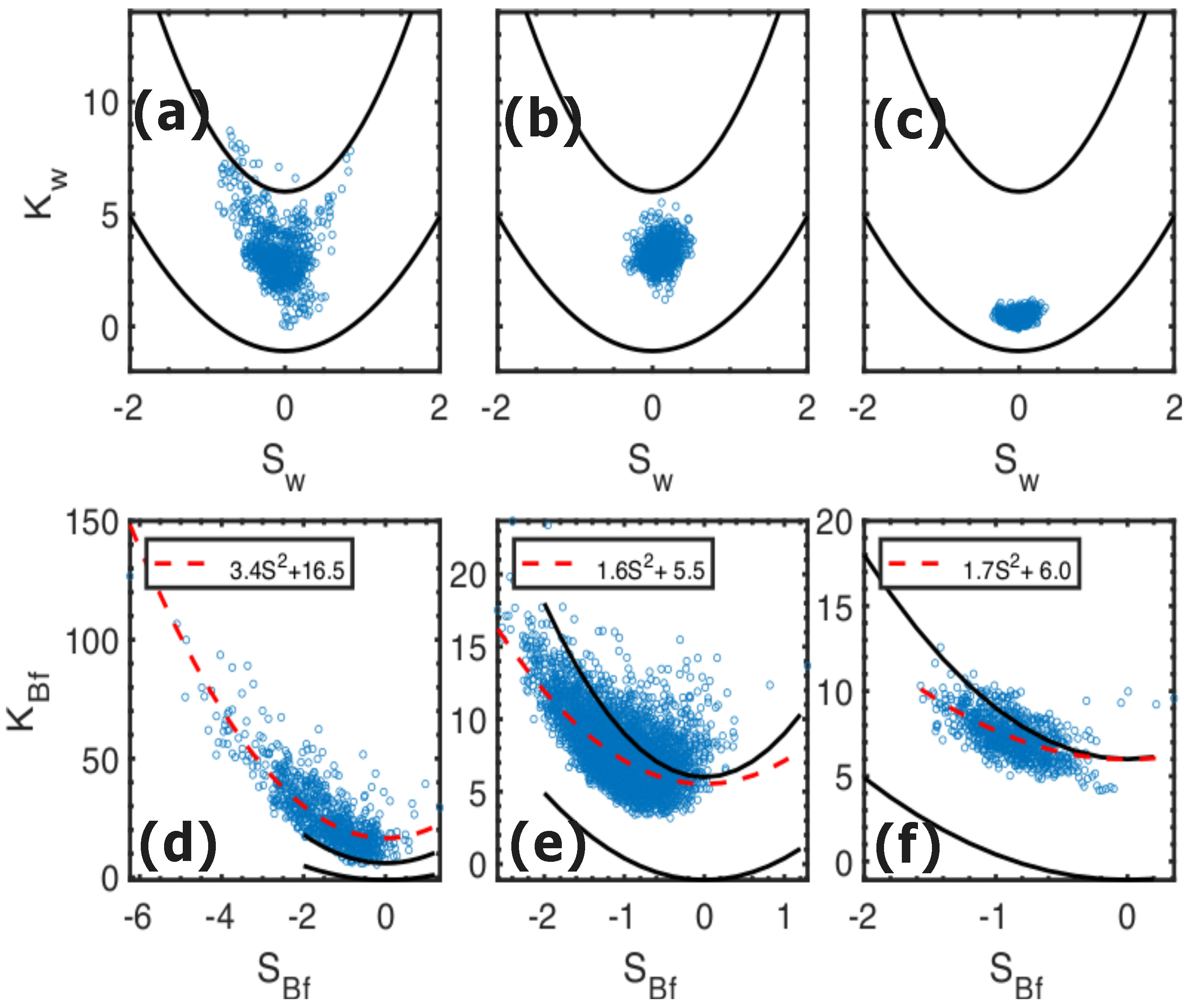
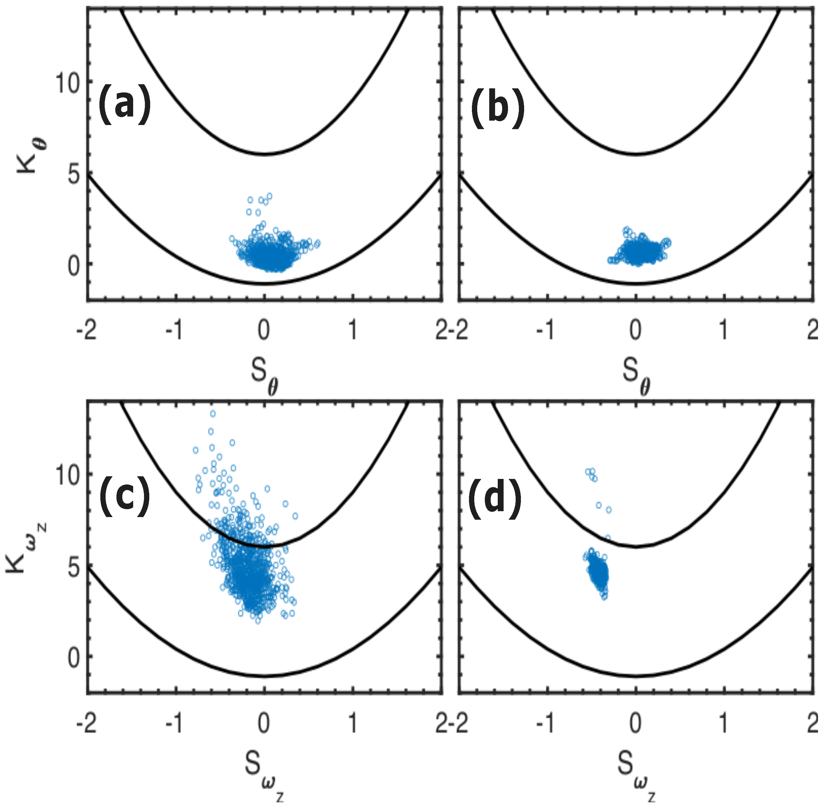
4. The Case of Rotating Stratified Turbulence (RST)

Intermittent vertical velocities are also found in RST, for decaying flows [74] and, as shown here, in forced runs. We look first at global dynamics. In Figure 3a is given as a function of time the total kinetic energy for run H1 as a base, and for three runs with varying F r and 0.36 R o 3.7 . The higher level of saturation for the RST runs is due to the fact that on the one hand, there is a lesser dissipation due to the strong effect of waves, and on the other hand, R o 0.36 for run Q1, which is low enough that an inverse transfer of energy to the large scales is plausible, although it cannot be distinguished directly on energy spectra which are still peaked at k k F (see Figure 3d). Higher R o may correspond to the environment of tropical storms in which turbulence also plays a dual role [131,132]. In Figure 3b we plot K w (dotted magenta line), the kinetic (solid blue), potential (black dashed) and total energy dissipation rates for run R1, with the time expressed in units of the turnover time τ N L . We see that K w can take large values, as in the purely stratified case [30]. There are also discernible excursions in the dissipation rates. The high-K values are associated with local instabilities and overturning regions; these excursions in K w are also present in several other runs. We recover here the behavior analyzed in detail in [30,31] for purely stratified flows: narrow peaks in K w as a function of F r and R B occur, compatible with observed strong updrafts in the DNS. The temporal evolution of the kinetic energy E V and enstrophy | ω | 2 are given for the total length of that run in (c), showing a persistence in the amplitude of fluctuations. The sporadic energetization of the flow has its signature in energy spectra shown in Figure 3d for run R1; indeed, the kinetic and potential spectra gain close to a factor of ten at the smallest scales for an excited state (with a peak in K w ) when compared to quiet times (with a trough in K w ), whereas the spectra have comparable amplitudes at the largest scales. Similar differences in small-scale spectra occur for the QG runs. Note also that, the forcing being centered in the large scales, no inverse cascade of energy that would occur in the presence of strong rotation can be observed in these runs (see [81,82] for DNS resolving both the inverse and direct energy cascades).
In Figure 4, we give K ( S ) for w for runs R1–R3 (a–c), and for B f for runs Q1, Q3, and Q8 (d–f), with buoyancy Reynolds numbers varying from 1.4 to 385. At top, the skewness is typically bounded by ± 1 or less, and there is a clear decrease in the kurtosis of the vertical velocity as R B increases from left to right. We note that, for all these runs, and similarly to the FDT and purely stratified cases, the vertical velocity has basically no skewness but its kurtosis can take moderate values, especially so at intermediate R B (here, the first plot), although no parabolic law emerges from the data. For the buoyancy flux, there is a marked transition towards a standard scaling ( 1.5 S 2 + b ), once the Kolmogorov regime is sufficiently resolved, i.e., for high enough R B , R i g , and with a classical FDT dissipation taking place (Figure 4e,f). Note that the intermittency uncovered in this paper likely deals more with intrinsic properties of dissipation than local accelerations that might be observed in a boundary layer. A different approach, following [109], is to expand the PDF in terms of its cumulant under the assumption of closeness to a Gaussian distribution. In the simplest case, a relationship is obtained, namely K = [ 4 S / 3 ] 2 , close to the previous expression ( a 1.5 for small b). The K ( S ) plots for the temperature (Figure 5a,b) and the vertical component of the vorticity (c,d plots in Figure 5) are similar as well, as shown for runs Q2 (a,c) and Q7 (b,d). In all cases, the skewness stays close to zero and there is a decrease of kurtosis as the flows become more dynamical.
A last issue is how much mixing occurs, estimated through B f , ϵ d u taken as proxies [79,86]. Thus, we give in Figure 6, K ( S ) for ϵ d u for runs Q1, Q2 (a,b) with R e s T 1 , and Q5, Q6 (d,e, R e s T > 10 ). Again, a transition is observed, with steeper scaling in the latter case; similar results obtain for FDT, with a best fit for ϵ d u (run H2) of K = 2.6 S 2 + 7.2 (not shown). Note that, for the components of the strain tensor itself, S i j = [ i u j + j u i ] / 2 , we have K 21 S 2 / 4 in the incompressible case [133]. Figure 6 (right) gives the PDFs of ϵ d u for run Q3 for times with a high (c) and low (f) K w ; a 3 power law is plausible, with a larger extension when the intermittency of w is stronger; note that a shallower scaling for ϵ d u has been observed in oceanic data, together with substantially higher values of K , S [134]. In the fits, α = 1 + S ϵ d u 2 / 4 (see [108]).

5. Possible Frameworks for K(S) Relationships

It is not clear what the link of the above results is with the analysis of complex turbulent flows using the concept of avalanches and of self-organized criticality [127,135]. In that latter case, the dissipative structures at small scale propagate in some fashion their intermittency to the large scales, just as small avalanches become large through merging. Saying it another way, dissipative structures near strain and vortices, or in current sheets and filaments, exist at the large scale characteristic of the flow and at the small scale corresponding to their thickness, of the order of the dissipation length. Therefore, the governing parameter may not be R e or R λ , but could be related to the ability of the small-scale structures to organize into larger clusters, or in other words to a transition at the local (in scale) Reynolds number of unity in the vicinity of the Kolmogorov scale in fluid turbulence. The occurrence of a quadratic K ( S ) law, albeit with varying coefficients, has been noted before. One should analyze large-enough samples [108,136]), but the non-Gaussianity of turbulence is ascertained, for non-vanishing dissipation, by the exact laws stemming from the conservation of quadratic invariants, as for kinetic energy in fluid turbulence [137,138], under several conditions:
δ u L 3 ( r ) = 4 5 ϵ d u r , δ u L ( r ) Σ i δ u i 2 ( r ) = 4 3 ϵ d u r ,
with u L the longitudinal velocity along the distance | r | , and δ expressing velocity differences. In MHD, cross-field correlations emerge [139] (see [140] for a review), which are central to the structure of reconnection events [33,47,141]. Inertia-gravity waves, which exchange energy between the kinetic and potential modes, will not alter the balance at the level of total energy dissipation. However, when writing an equation for the temporal evolution of B f , it occurs at the scale of the turn-over time since it deals with large-scale variables, whereas the equipartition deficiency N [ θ 2 w 2 ] due to waves evolves on a fast time for small F r and can be averaged to be modeled as a stochastic forcing for B f , ϵ d u ; this makes their temporal evolutions akin to systems already discussed herein (see e.g., [38,119]).
Another remark is that, obtaining quadratic K ( S ) laws for both weak and strong turbulence, diffusive or not, and dispersive or not, could lead one to conclude that the issue is more of a mathematical constraint than a physical one. However, the K ( S ) relationship is important in limiting possible closures applied to turbulence, as for example in the context of solar convection (see [107] for recent developments of closures beyond the quasi-normal framework). It has also been remarked that these systems have in common a convective nonlinearity, however weak or intense [97]. The specific transition in the scaling of the K ( S ) laws obtained here is linked to the fact that waves become progressively more strongly coupled to nonlinear eddies, or in other words steepen significantly, thus leading to enhanced dissipation and to the onset of a Kolmogorov energy spectrum at small scale. The existence of K S 2 laws at high and low R λ leads to another possible origin for it, namely the presence of intermittency in the dissipation range common to all such flows. As pointed out in [15,142], this range can be prone to extreme intermittency because of a faster than algebraic decrease of the intensity of turbulence at high wavenumber, a spectral domain that exists even in the near absence of a nonlinear inertial range at low R λ . This likely leaves only a few shear structures dominating the overall statistics. In this context, studies of Lagrangian turbulence have been able to show the link between the dissipation range and large scales, with both short and long-range correlations [143].
Computations performed at moderate R λ identify small-scale intermittency with numerous large-scale structures [15], as opposed to the more familiar vortex filaments [144,145,146]. Such nonlocal structures could be detected in rotating stratified flows using specific algorithms (see [135] for the identification of current sheets at the onset of the dissipation range of plasmas in the MHD regime). In that spirit, it would be of interest to consider as well the case of quasi-geostrophy, that of cubic nonlinearities like for compressible flows, or for solitons (such as for the Korteweg–deVries or the cubic nonlinear Schrödinger (NLS) equations and their multi-dimensional extensions), all in the presence of forcing and dissipation (see also [147] where the K ( S ) behavior for the NLS equation is associated with on-off intermittency). The large-scale behavior linked with the presence of Rossby waves and their possible nonlinear coupling and breaking may also reinforce or even alter large-scale intermittency.
Finally, a link between inertial and dissipative ranges is consistent with a linear stochastic model for the fast small scales which is successful in giving K ( S ) S 2 for climate data [38,39]. In decaying experiments at both low and high R λ using sulfur hexafluoride, the inertial range does not follow a strict power-law, but rather may display a logarithmic correction that is independent of Reynolds number and that may arise from the dissipative range, putting into question their independence [148]. Nonlinearities do not seem to be central to the establishment of non-Gaussian statistics beyond their (necessary) mode-coupling role [149], and it is rather the susceptibility of the system being close to criticality, linking all scales through dissipation that is central to turbulence dynamics and intermittency. This can manifest itself as avalanches in granular media, or in the development of shear instabilities in (e.g., RST) flows close to the critical Richardson number ([74,75,89,127,150] and references therein).

6. Discussion, Conclusions, and Perspectives

In the nocturnal planetary boundary layer, “… turbulence is expected to become more intermittent in very stable conditions“ (Mahrt et al. [52]). Relating to these observations, we are likely dealing in this paper with two phenomena, possibly superposed and intertwined. On the one hand, we have the increased intermittency, as diagnosed by a high kurtosis of vertical velocity and temperature, if in a narrow domain of Froude and buoyancy Reynolds number [30,74], and signaling the onset of small-scale turbulence interacting with the larger-scale (inertia)-gravity waves. The signature in physical space consists of a high local vertical velocity and hence a high local Reynolds number, allowing for instabilities to develop until the system evolves (in a turn-over time) back to a state dominated by the fast waves [31,127,130,151], and the cycle can restart. Thus, it leads to strong local energy dissipation in an otherwise wave-dominated rather placid system, and as such these isolated hot spots are a critical factor in controlling the overall dissipation. This dynamics can be modeled e.g., through the temporal evolution of the velocity and temperature gradient matrices, taking into account the anisotropy of the system and using a closure for the pressure Hessian [130]. High kurtosis values for the vertical velocity are narrowly centered around a peak in Froude number (and in R I B ), although it is not known at this point how much the peak depends on the Reynolds number itself. They can be associated for example with jet meandering in the ocean and modeled through stochastic parametrization. In fact, it has been hypothesized—and studied in depth over the years—that shear flows are central to the critical instability of turbulence, a point further developed recently in a global fluid context [152,153,154,155], and applied to stratified fluids as well [127] (see [128] for RST, and [156] for plasmas). This transition could also be linked to a role-change in potential vorticity P V at small scales due to the breaking, at the Ozmidov scale onward, of gravity waves [80].
On the other hand, different K ( S ) laws emerge with different coefficients for the buoyancy flux, the kinetic energy dissipation as well as for mixing as measured through the ratio B f / ϵ d u . This second phenomenon of a transition between regimes for K ( S ) is new to our knowledge, certainly in the specific context of rotating stratified flows, but of course long computations at higher R e , R I B with a resolved range beyond O z are needed. The scaling corresponds to a shift, in the small scales and possibly as well in the early dissipation range, in the nature of an intermittency which becomes stronger as the nonlinear eddies get stronger, and with a K ( S ) scaling for B f which seems to approach that found for other turbulent systems [38,41,46]. This is linked to the well-known transition at the Ozmidov scale of an energy spectrum becoming progressively more Kolmogorov-like. Many models have been proposed for these K ( S ) parabolic laws, as partially reviewed all along in the paper. More work will be needed to sort out the different possibilities, and to reach higher buoyancy Reynolds numbers corresponding to conditions pertaining to those in atmospheric and oceanic flows. In order to obtain dissipative structures at higher R B for long-time runs, a computation in a non-cubic geometry will help tremendously. For example, it was shown in [157] that in a flat box with a 1:8 aspect ratio, the process of front and filament formation can be very efficient in sheared flows [130]. The evolution of extreme events in such flows with comparable geometries was also considered in [158] for their effect on the mixing of neutrally buoyant particles (see also [159] for a substantially higher aspect ratio together with using hyper-viscosity). Similarly, peak vertical vorticity can be close to two orders of magnitude larger than the imposed rotation, as shown in [160] within a Large Eddy Simulation (LES) framework. Another feature of these flows is their persistent anisotropy [59,128,161,162], associated, for example, with seasonal oceanic variability [163]. Thus, the precise formulation of the small-scale parametrization and of the dissipation of resolved scales in numerical codes may affect the mesoscale dynamical properties such as energy spectra [164]. Related evaluations for plasma disruptions and fusion, from MHD to Hall-MHD and beyond, might also be of interest to understand better– and possibly control to some extent– these strong small-scale disruptive features.
One of the several models of dissipative events leading to a quadratic K ( S ) relationship not yet mentioned here is in the context of so-called 1 / f n noise as a signature of long-time correlations in turbulent hydrodynamic and MHD flows [165] where it is shown that the transition from Gaussian statistics in the inviscid case to a non-Gaussian one in the presence of dissipation can be associated with varying properties of energy transfer through scales. Are there several different classes of universality, though? In this context, we have already noted that, for the Navier–Stokes equations, there is a clear departure from standard coefficients for the law K ( S ) = 3 S 2 / 2 1.1 , as well as for low Froude numbers in the case of stratified turbulence and RST.
Another potential issue is the form of the dissipation operator. When using either eddy viscosity or hyper-viscosity as a model, or LES, a sub-grid scale algorithm, or the α -model Lagrangian description for fluids and MHD, do similar quadratic K ( S ) relations arise? What about for the cyclostrophic balance in helical stratified flows [166]? Or in the ideal ( ν = 0 ) case in its pseudo-dissipative range stemming from the eddy viscosity due to the small-scale equilibrium range [167], or in 2D MHD or even in 1D (allowing for the long temporal integrations which are needed in this intermediate inviscid but turbulence-like phase)? In other words, does modifying the way energy is dissipated in turbulence alter the K ( S ) relation for velocity or dissipation, therefore suggesting that it is a crucial feature for dissipative events? We already know that the PDFs of velocity gradients in the NS case are affected [168], but it is not clear whether the K ( S ) law would be. Such renormalized dissipation arise at high R e , whereas a K S 2 relation is present as well at moderate R e , for which the viscosity is directly active. If a change in the K ( S ) law occurs, beyond the one identified in this paper and related to the onset of a Kolmogorov range beyond O z , what functional form does it take, and are there consequences for accuracy in an evaluation of the large-scale dynamics that weather and climate codes seek to reproduce faithfully while using techniques such as LES (see, e.g., the discussion in [108])?
We have presented preliminary results, limited in Reynolds number, and much remains to be done. One issue is to examine the dual constant-flux energy cascade when forcing is at smaller scale [81,82]. Other questions arise, such as the persistence of large-scale intermittency of vertical velocity in RST in the presence of a resolved turbulence range, or of strong helicity (see e.g., [169,170] on intermittency and helicity in FDT). Nonlinear interactions u × ω are weakened in vortex tubes, potentially allowing waves to play a more prominent role in driving the flow closer to the critical state in which strong vertical drafts and ensuing dissipation occur. A wave-vortex decomposition, such as that studied e.g., in [171,172], could be of help to distinguish between these different regimes. One can also ask how anisotropy in RST flows is affected by these strong updrafts. Large-scale intermittency has also been linked to the role of helicity (velocity-vorticity correlations) [173], and the eigenvectors of strain can play an important role as well in intermittent energy transfer, as shown in a simple model in which alignment of vorticity with strain eigenvector corresponding at first to its intermediate eigenvalue, and featuring the combination of a shear flow with a horizontal straining field [174] (see also [175]), and yet anisotropy is essential in possibly stopping the formation of singular structures [70].
We wish to end this text with a direct quote from a review article on waves and coherent flows in the tropics (Stephan et al. [176], see page 2619): “Theory provides the qualitative framework—the causal narrative—within which the quantitative information from models and observations can be meaningfully compared and usefully combined.” The research of Jack Herring was on the idealized, theoretical side of the study of the dynamics of the atmosphere, pioneering the inclusive use of theoretical and numerical approaches. As such, it has provided invaluable information, and causal accounts, for the idealized behavior of turbulence and the central role played by nonlinear effects in such—and other geophysical, astrophysical as well as engineering, chemical, biological and climatological—complex systems.

Author Contributions

All authors contributed equally on all aspects of this paper. All authors have read and agreed to the published version of the manuscript.

Funding

Duane Rosenberg acknowledges support from award NOAA/OAR/NA19OAR4320073. Raffaele Marino acknowledges support from the project EVENTFUL (ANR-20-CE30-0011), funded by the French Agence Nationale de la Recherche-ANR through the program AAPG-2020.

Data Availability Statement

Data is available for all runs from the authors upon request.

Acknowledgments

We all would like to express our gratitude to Jack Herring, and acknowledge many enlightening discussions with him over our years at the Geophysical Turbulence Program which Jack helped create at NCAR, and which was extremely successful in the turbulence community at large. His interest in pursuing and encouraging colleagues to pursue a theoretical understanding of turbulence in atmospheric and geophysical flows in general never waned, nor did his kindness to others and his open-mindedness. Finally, Annick Pouquet is thankful to LASP (University of Colorado at Boulder), and in particular to Bob Ergun.

Conflicts of Interest

The authors declare no conflict of interest.

References

  1. Kraichnan, R. The structure of isotropic turbulence at very high Reynolds numbers. J. Fluid Mech. 1959, 5, 497–543. [Google Scholar] [CrossRef]
  2. Sukoriansky, S.; Galperin, B.; Staroselsky, I. A quasinormal scale elimination model of turbulent flows with stable stratification. Phys. Fluids 2005, 17, 085107. [Google Scholar] [CrossRef]
  3. Nazarenko, S. Wave Turbulence; Lecture Notes in Physics; Springer: Berlin/Heidelberg, Germany, 2011; Volume 825. [Google Scholar]
  4. Zhou, Y. Turbulence theories and statistical closure approaches. Phys. Rep. 2021, 935, 1–117. [Google Scholar]
  5. Marston, J.B.; Tobias, S.M. Recent Developments in Theories of Inhomogeneous and Anisotropic Turbulence. Ann. Rev. Fluid Mech. 2022, 55, 1–29. [Google Scholar] [CrossRef]
  6. Lorenz, E.N. The predictability of a flow which possesses many scales of motion. Tellus 1969, 21, 289–307. [Google Scholar] [CrossRef]
  7. Leith, C.; Kraichnan, R. Predictability of turbulent flows. J. Atmos. Sci. 1972, 29, 1041–1058. [Google Scholar] [CrossRef]
  8. Herring, J.R.; Riley, J.J.; Patterson, G.S., Jr.; Kraichnan, R.H. Growth of Uncertainty in Decaying Isotropic Turbulence. J. Atm. Sci. 1973, 30, 997–1006. [Google Scholar] [CrossRef]
  9. Herring, J.R. Approach of axisymmetric turbulence to isotropy. Phys. Fluids 1974, 17, 859–872. [Google Scholar] [CrossRef]
  10. Schumann, U.; Herring, J. Axisymmetric homogeneous turbulence: A comparison of direct spectral simulations with the direct-interaction approximation. J. Fluid Mech. 1976, 76, 755–782. [Google Scholar] [CrossRef]
  11. Herring, J.R. Statistical theory of quasi-geostrophic turbulence. J. Atmos. Sci. 1980, 37, 969–977. [Google Scholar] [CrossRef]
  12. Herring, J.R.; Kerr, R.M. Comparison of direct numerical simulations with predictions of two-point closures for isotropic turbulence convecting a passive scalar. J. Fluid Mech. 1982, 118, 205–219. [Google Scholar] [CrossRef]
  13. Herring, J.; McWilliams, J. Comparison of direct numerical simulations of two-dimensional turbulence with two-point closure: The effects of intermittency. J. Fluid Mech. 1985, 153, 229–242. [Google Scholar] [CrossRef]
  14. Chen, H.; Herring, J.R.; Kerr, R.M.; Kraichnan, R.H. Non-Gaussian statistics in isotropic turbulence. Phys. Fluids 1989, A1, 1844–1855. [Google Scholar] [CrossRef]
  15. Chen, S.; Doolen, G.; Herring, J.R.; Kraichnan, R.H.; Orszag, S.A.; She, Z.S. Far-Dissipation Range of Turbulence. Phys. Rev. Lett. 1993, 70, 3051–3054. [Google Scholar] [CrossRef]
  16. Métais, O.; Herring, J. Numerical simulations of freely evolving turbulence in stably stratified fluids. J. Fluid Mech. 1989, 202, 117–148. [Google Scholar] [CrossRef]
  17. Kimura, Y.; Herring, J. Diffusion in stably stratified turbulence. J. Fluid Mech. 1996, 328, 253–269. [Google Scholar] [CrossRef]
  18. Champagne, F. The fine-scale structure of the turbulent velocity field. J. Fluid Mech. 1978, 86, 67–108. [Google Scholar] [CrossRef]
  19. Buaria, D.; Bodenschatz, E.; Pumir, A. Vortex stretching and enstrophy production in high Reynolds number turbulence. Phys. Rev. F 2020, 5, 104602. [Google Scholar] [CrossRef]
  20. Klymak, J.M.; Pinkel, R.; Rainville, L. Direct Breaking of the Internal Tide near Topography: Kaena Ridge, Hawaii. J. Phys. Oceano. 2008, 38, 380–399. [Google Scholar] [CrossRef]
  21. Belonenko, T.V.; Sandalyuk, N.V.; Gnevyshev, V.G. Interaction of Rossby waves with the Gulf Stream and Kuroshio using altimetry in a framework of a vortex layer model. Adv. Space Res. 2023, 71, 2384–2393. [Google Scholar] [CrossRef]
  22. Davis, A.Y.; Yan, X.H. Hurricane forcing on chlorophyll-a concentration off the northeast coast of the U.S. Geophys. Res. Lett. 2004, 31, L17304. [Google Scholar] [CrossRef]
  23. Grisouarda, N.; Leclair, M.; Gostiaux, L.; Staquet, C. Large-scale energy transfer from an internal gravity wave reflecting on a simple slope. Proc. IUTAM 2013, 8, 119–128. [Google Scholar] [CrossRef]
  24. McWilliams, J.C. A survey of submesoscale currents. Geosci. Lett. 2019, 6, 3. [Google Scholar] [CrossRef]
  25. Chau, J.; Marino, R.; Feraco, F.; Urco, J.; Baumgarten, G.; Lubken, F.; Hocking, W.; Schult, C.; Renkwitz, T.; Latteck, R. Radar observation of extreme vertical drafts in the polar summer mesosphere. Geophys. Res. Lett. 2021, 48, e2021GL094918. [Google Scholar] [CrossRef]
  26. Nastrom, G.D.; Gage, K. A climatology of atmospheric wavenumber spectra of wind and temperature observed by commercial aircraft. J. Atmos. Sci. 1985, 42, 950–960. [Google Scholar] [CrossRef]
  27. Waite, M.L. Random forcing of geostrophic motion in rotating stratified turbulence. Phys. Fluids 2017, 29. [Google Scholar] [CrossRef]
  28. Mininni, P.D.; Pouquet, A. Energy spectra stemming from interactions of Alfvén waves and turbulent eddies. Phys. Rev. Lett. 2007, 99, 254502. [Google Scholar] [CrossRef]
  29. Matthaeus, W. Turbulence in space plasmas: Who needs it? Phys. Plasmas 2021, 28, 032306. [Google Scholar] [CrossRef]
  30. Feraco, F.; Marino, R.; Pumir, A.; Primavera, L.; Mininni, P.; Pouquet, A.; Rosenberg, D. Vertical drafts and mixing in stratified turbulence: Sharp transition with Froude number. Eur. Phys. Lett. 2018, 123, 44002. [Google Scholar] [CrossRef]
  31. Marino, R.; Feraco, F.; Primavera, L.; Pumir, A.; Pouquet, A.; Rosenberg, D. Turbulence generation by large-scale extreme drafts and the modulation of local energy dissipation in stably stratified geophysical flows. Phys. Rev. F 2022, 7, 033801. [Google Scholar] [CrossRef]
  32. Osman, K.; Matthaeus, W.H.; Wand, M.; Rapazzo, A. Intermittency and local heating in the solar wind. Phys. Rev. Lett. 2012, 108, 261102. [Google Scholar] [CrossRef] [PubMed]
  33. Ergun, R.E.; Goodrich, K.A.; Wilder, F.D.; Ahmadi, N.; Holmes, J.C.; Eriksson, S.; Stawarz, J.E.; Nakamura, R.; Genestreti, K.J.; Hesse, M.; et al. Magnetic Reconnection, Turbulence, and Particle Acceleration: Observations in the Earth’s Magnetotail. Geophys. Res. Lett. 2018, 45, 3338–3347. [Google Scholar] [CrossRef]
  34. Lenschow, D.; Mann, J.; Kristensen, L. How long is long enough when measuring fluxes and other turbulence statistics? J. Atm. Oc. Tech. 1994, 11, 661–673. [Google Scholar] [CrossRef]
  35. Mole, N.; Clarke, E. Relationships between higher moments of concentration and of dose in turbulent dispersion. Bound. Layer Met. 1995, 73, 35–52. [Google Scholar] [CrossRef]
  36. Lewis, D.; Chatwin, P.; Mole, N. Investigation of the collapse of the skewness and kurtosis exhibited in atmospheric dispersion data. Nuovo Cimento 1997, 20, 385–397. [Google Scholar]
  37. Schopflocher, L.; Sullivan, P.J. The relationship between skewness and kurtosis of a diffusing scalar. Bound. Layer Met. 2005, 115, 341–358. [Google Scholar] [CrossRef]
  38. Sura, P.; Sardeshmukh, P.D. A global view of non-Gaussian SST variability. J. Phys. Oceano. 2008, 38, 639–647. [Google Scholar] [CrossRef]
  39. Sardeshmukh, P.D.; Sura, P. Reconciling Non-Gaussian Climate Statistics with Linear Dynamics. J. Climate 2009, 22, 1193–1207. [Google Scholar] [CrossRef]
  40. Kaur, S.; Lukovich, J.V.; Ehn, J.K.; Barber, D.G. Higher-order statistical moments to analyse Arctic sea-ice drift patterns. Ann. Glaciology 2021, 61, 464–471. [Google Scholar] [CrossRef]
  41. Labit, B.; Furno, I.; Fasoli, A.; Diallo, A.; Müller, S.; Plyushchev, G.; Podestà, M.; Poli, F. Universal Statistical Properties of Drift-Interchange Turbulence in TORPEX Plasmas. Phys. Rev. Lett. 2007, 98, 255002. [Google Scholar] [CrossRef]
  42. Krommes, J.A. The remarkable similarity between the scaling of kurtosis with squared skewness for TORPEX density fluctuations and sea-surface temperature fluctuations. Phys. Plasmas 2008, 15, 030703. [Google Scholar] [CrossRef]
  43. Sattin, F.; Agostini, M.; Cavazzana, R.; Serianni, G.; Scarin, P.; Vianello, N. About the parabolic relation between the skewness and the kurtosis in time series of experimental data. Phys. Scrip. 2009, 79, 045006. [Google Scholar] [CrossRef]
  44. Burkhart, B.; Stanimirovic, S.; Lazarian, A.; Kowal, G. Characterizing magnetohydrodynamic turbulence in the small Magellanic cloud. Astrophys. J. 2010, 708, 1204–1210. [Google Scholar] [CrossRef]
  45. Hamza, A.; Meziane, K. On turbulence in the quasi-perpendicular bow shock. Planet. Space Sci. 2011, 59, 475–481. [Google Scholar] [CrossRef]
  46. Osmane, A.; Dimmock, A.; Pulkkinen, T. Universal properties of mirror mode turbulence in the Earth magnetosheath. Geophys. Res. Lett. 2015, 42, 3085–3092. [Google Scholar] [CrossRef]
  47. Miranda, R.A.; Schelin, A.B.; Chian, A.C.L.; Ferreira, J.L. Non-Gaussianity and cross-scale coupling in interplanetary magnetic field turbulence during a rope-rope magnetic reconnection event. Ann. Geophys. 2018, 36, 497–507. [Google Scholar] [CrossRef]
  48. Maier, E.; Elmegreen, B.G.; Hunter, D.A.; Chien, L.H.; Hollyday, G.; Simpson, C.E. The Nature of Turbulence in the LITTLE THINGS Dwarf Irregular Galaxies. Astrophys. J. 2017, 153, 163. [Google Scholar] [CrossRef]
  49. Rosenberg, D.; Pouquet, A.; Marino, R.; Mininni, P. Evidence for Bolgiano-Obukhov scaling in rotating stratified turbulence using high-resolution direct numerical simulations. Phys. Fluids 2015, 27, 055105. [Google Scholar] [CrossRef]
  50. Kafiabad, H.; Bartello, P. Balance dynamics in rotating stratified turbulence. J. Fluid Mech. 2016, 795, 914–949. [Google Scholar] [CrossRef]
  51. Pouquet, A.; Rosenberg, D.; Marino, R.; Herbert, C. Scaling laws for mixing and dissipation in unforced rotating stratified turbulence. J. Fluid Mech. 2018, 844, 519–545. [Google Scholar] [CrossRef]
  52. Mahrt, L.; Sun, J.; Blumen, W.; Delany, T.; Oncley, S. Nocturnal boundary-layer regimes. Bound. Lay. Met. 1998, 88, 255–278. [Google Scholar] [CrossRef]
  53. Brethouwer, G.; Billant, P.; Lindborg, E.; Chomaz, J.M. Scaling analysis and simulation of strongly stratified turbulent flows. J. Fluid Mech. 2007, 585, 343–368. [Google Scholar] [CrossRef]
  54. Laval, J.P.; McWilliams, J.; Dubrulle, B. Forced stratified turbulence: Successive transitions with Reynolds number. Phys. Rev. E 2003, 68, 036308. [Google Scholar] [CrossRef] [PubMed]
  55. Legaspi, J.D.; Waite, M.L. Prandtl number dependence of stratified turbulence. J. Fluid Mech. 2020, 903, A12. [Google Scholar] [CrossRef]
  56. Venayagamoorthy, S.; Koseff, J. On the flux Richardson number in stably stratified turbulence. J. Fluid Mech. 2016, 798, R1–R10. [Google Scholar] [CrossRef]
  57. Oks, D.; Mininni, P.; Marino, R.; Pouquet, A. Inverse cascades and resonant triads in rotating and stratified turbulence. Phys. Fluids 2017, 29, 111109. [Google Scholar] [CrossRef]
  58. Lelong, M.P.; Riley, J. Internal wave-vortical mode interactions in strongly stratified flows. J. Fluid Mech. 1991, 232, 1–19. [Google Scholar] [CrossRef]
  59. Sukoriansky, S.; Galperin, B. An analytical theory of the buoyancy-Kolmogorov subrange transition in turbulent flows with stable stratification. Phil. Trans. Roy. Soc. A 2013, 371, 20120212. [Google Scholar] [CrossRef]
  60. Falcon, E.; Aumaitre, S.; Falcon, C.; Laroche, C.; Fauve, S. Fluctuations of Energy Flux in Wave Turbulence. Phys. Rev. Lett. 2008, 100, 064503. [Google Scholar] [CrossRef]
  61. Lee, J.S.; Kwon, C.; Park, H. Everlasting initial memory threshold for rare events in equilibration processes. Phys. Rev. E 2013, 87, 020104. [Google Scholar] [CrossRef]
  62. Sukoriansky, S.; Galperin, B. QNSE theory of turbulence anisotropization and onset of the inverse energy cascade by solid body rotation. J. Fluid Mech. 2016, 805, 384–421. [Google Scholar] [CrossRef]
  63. Rosenberg, D.; Mininni, P.D.; Reddy, R.; Pouquet, A. GPU Parallelization of a Hybrid Pseudospectral Geophysical Turbulence Framework Using CUDA. Atmosphere 2020, 11, 178. [Google Scholar] [CrossRef]
  64. Fontana, M.; Bruno, O.P.; Mininni, P.D.; Dmitruk, P. Fourier continuation method for incompressible fluids with boundaries. Comp. Phys. Comm. 2020, 256, 107482. [Google Scholar] [CrossRef]
  65. Godeferd, F.; Cambon, C. Detailed investigation of energy transfers in homogeneous stratified turbulence. Phys. Fluids 1994, 6, 2084–2100. [Google Scholar] [CrossRef]
  66. Rorai, C.; Mininni, P.; Pouquet, A. Stably stratified turbulence in the presence of large-scale forcing. Phys. Rev. E 2015, 92, 013003. [Google Scholar] [CrossRef] [PubMed]
  67. Hughes, C.W.; Thompson, A.F.; Wilson, C. Identification of jets and mixing barriers from sea level and vorticity measurements using simple statistics. Ocean Mod. 2010, 32, 44–57. [Google Scholar] [CrossRef]
  68. Yakhot, V.; Donzis, D.A. Anomalous exponents in strong turbulence. Phys. D 2018, 384, 12. [Google Scholar] [CrossRef]
  69. Khurshid, S.; Donzis, D.A.; Sreenivasan, K.R. Emergence of universal scaling in isotropic turbulence. Phys. Rev. E 2023, 107, 045102. [Google Scholar] [CrossRef]
  70. Bradshaw, Z.; Farhat, A.; Grujic, Z. An Algebraic Reduction of the Scaling Gap in the Navier-Stokes Regularity Problem. Arch. Ration. Mech. Anal. 2019, 231, 1983–2005. [Google Scholar] [CrossRef]
  71. Rafner, J.; Grujic, Z.; Bach, C.; Bærentzen, J.A.; Gervang, B.; Jia, R.; Leinweber, S.; Misztal, M.; Sherson, J. Geometry of turbulent dissipation and the Navier-Stokes regularity problem. Sci. Rep. 2021, 11, 8824. [Google Scholar] [CrossRef]
  72. Buaria, D.; Pumir, A.; Bodenschatz, E. Generation of intense dissipation in high Reynolds number turbulence. Phil. Trans. A 2022, 380, 20210088. [Google Scholar] [CrossRef] [PubMed]
  73. Rorai, C.; Mininni, P.; Pouquet, A. Turbulence comes in bursts in stably stratified flows. Phys. Rev. E 2014, 89, 043002. [Google Scholar] [CrossRef] [PubMed]
  74. Rosenberg, D.; Pouquet, A.; Marino, R. Correlation between buoyancy flux, dissipation and potential vorticity in rotating stratified turbulence. Atmosphere 2021, 12, 157. [Google Scholar] [CrossRef]
  75. Pouquet, A.; Rosenberg, D.; Stawarz, J.; Marino, R. Helicity Dynamics, Inverse, and Bidirectional Cascades in Fluid and Magnetohydrodynamic Turbulence: A Brief Review. Earth Space Sci. 2019, 6, 1–19. [Google Scholar] [CrossRef]
  76. Tuckerman, L.S.; Chantry, M.; Barkley, D. Patterns in Wall-Bounded Shear Flows. Ann. Rev. Fluid Mech. 2020, 52, 343–367. [Google Scholar] [CrossRef]
  77. McWilliams, J.C. Submesoscale currents in the ocean. Proc. Roy. Soc. A 2016, 472, 20160117. [Google Scholar] [CrossRef]
  78. Legg, S. Mixing by Oceanic Lee Waves. Ann. Rev. Fluid Mech. 2021, 53, 173–201. [Google Scholar] [CrossRef]
  79. Caulfield, C.P. Layering, Instabilities, and Mixing in Turbulent Stratified Flows. Ann. Rev. Fluid Mech. 2021, 53, 113–145. [Google Scholar] [CrossRef]
  80. Waite, M.L.; Richardson, N. Potential Vorticity Generation in Breaking Gravity Waves. Atmosphere 2023, 14, 881. [Google Scholar] [CrossRef]
  81. Pouquet, A.; Marino, R. Geophysical turbulence and the duality of the energy flow across scales. Phys. Rev. Lett. 2013, 111, 234501. [Google Scholar] [CrossRef]
  82. Marino, R.; Pouquet, A.; Rosenberg, D. Resolving the paradox of oceanic large-scale balance and small-scale mixing. Phys. Rev. Lett. 2015, 114, 114504. [Google Scholar] [CrossRef] [PubMed]
  83. Faranda, D.; Lembo, V.; Iyer, M.; Kuzzay, D.; Chibbaro, S.; Daviaud, F.; Dubrulle, B. Computation and Characterization of Local Subfilter-Scale Energy Transfers in Atmospheric Flows. J. Atmos. Sci. 2018, 75, 2175–2186. [Google Scholar] [CrossRef]
  84. Wang, Y.; Brasseur, G.P.; Wang, T. Segregation of Atmospheric Oxidants in Turbulent Urban Environments. Atmosphere 2022, 13, 315. [Google Scholar] [CrossRef]
  85. Falgarone, E.; Pety, J.; Hily-Blandt, J. Intermittency of interstellar turbulence: Extreme velocity-shears and CO emission on milliparsec scale. Astron. Astrophys. 2009, 507, 355–368. [Google Scholar] [CrossRef]
  86. Cael, B.; Mashayek, A. Log-Skew-Normality of Ocean Turbulence. Phys. Rev. Lett. 2021, 126, 224502. [Google Scholar] [CrossRef]
  87. Elsinga, G.E.; Ishihara, T.; Hunt, J.C. Extreme dissipation and intermittency in turbulence at very high Reynolds number. Proc. Roy. Soc. A 2020, 476, 20200591. [Google Scholar] [CrossRef]
  88. Moeng, C.; Rotunno, R. Vertical velocity skewness in the buoyancy-driven boundary layer. J. Atmos. Sci. 1990, 47, 1149–1162. [Google Scholar] [CrossRef]
  89. Kit, E.; Hocut, C.M.; Liberzon, D.; Fernando, H.J.S. Fine-scale turbulent bursts in stable atmospheric boundary layer in complex terrain. J. Fluid Mech. 2017, 833, 745–772. [Google Scholar] [CrossRef]
  90. de Vries, A.J. A global climatological perspective on the importance of Rossby wave breaking and intense moisture transport for extreme precipitation events. Weather Clim. Dyn. 2021, 2, 129–161. [Google Scholar] [CrossRef]
  91. White, R.H.; Kai Kornhuber, O.M.; Wirth, V. From Atmospheric Waves to Heatwaves: A Waveguide Perspective for Understanding and Predicting Concurrent, Persistent, and Extreme Extratropical Weather. BAMS 2022, 103, E923–E935. [Google Scholar] [CrossRef]
  92. Petoukhov, V.; Rahmstorf, S.; Petri, S.; Schellnhuber, H.J. Quasiresonant amplification of planetary waves and recent Northern Hemisphere weather extremes. Proc. Nat. Acad. Sci. USA 2013, 110, 5336–5341. [Google Scholar] [CrossRef] [PubMed]
  93. Raphaldini, B.; Peixoto, P.S.; Teruya, A.S.W.; Raupp, C.F.M.; Bustamante, M.D. Precession resonance of Rossby wave triads and the generation of low-frequency atmospheric oscillations. Phys. Fluids 2022, 34, 076604. [Google Scholar] [CrossRef]
  94. Wirth, V.; Riemer, M.; Chang, E.K.; Martius, O. Rossby Wave Packets on the Midlatitude Waveguide—A Review. Month. Wea. Rev. 2018, 146, 1965–2001. [Google Scholar] [CrossRef]
  95. Antokhina, O.; Antokhin, P.; Gochakov, A.; Zbirannik, A.; Gazimov, T. Atmospheric Circulation Patterns Associated with Extreme Precipitation Events in Eastern Siberia and Mongolia. Atmosphere 2023, 14, 480. [Google Scholar] [CrossRef]
  96. Lenschow, D.H.; Lothon, M.; Mayor, S.D.; Sullivan, P.P.; Canut, G. A Comparison of Higher-Order Vertical Velocity Moments in the Convective Boundary Layer from Lidar with in Situ Measurements and Large-Eddy Simulation. Bound. Lay. Met. 2012, 143, 107–123. [Google Scholar] [CrossRef]
  97. Sandberg, I.; Benkadda, S.; Garbet, X.; Ropokis, G.; Hizanidis, K.; del Castillo-Negrete, D. Universal Probability Distribution Function for Bursty Transport in Plasma Turbulence. PRL 2009, 103, 165001. [Google Scholar] [CrossRef]
  98. Guszejnov, D.; Lazanyi, N.; Bencze, A.; Zoletnik, S. On the effect of intermittency of turbulence on the parabolic relation between skewness and kurtosis in magnetized plasmas. Phys. Plasma 2013, 20, 112305. [Google Scholar] [CrossRef]
  99. Fritts, D.C.; Werne, J. Stratified shear turbulence: Evolution and statistics. Geophys. Res. Lett. 2009, 26, 439–442. [Google Scholar]
  100. Thalabard, S.; Bec, J.; Mailybaev, A.A. From the butterfly effect to spontaneous stochasticity in singular shear flows. Comm. Phys. 2020, 122, 3. [Google Scholar] [CrossRef]
  101. Mininni, P.; Alexakis, A.; Pouquet, A. Nonlocal interactions in hydrodynamic turbulence at high Reynolds numbers: The slow emergence of scaling laws. Phys. Rev. E 2008, 77, 036306. [Google Scholar] [CrossRef]
  102. Tamarin-Brodsky, T.; Hodges, K.; Hoskins, B.J.; Sheperd, T.G. A Simple Model for Interpreting Temperature Variability and Its Higher-Order Changes. J. Clim. 2022, 35, 387–403. [Google Scholar]
  103. Sreenivasan, K.; Antonia, R.A. The phenomenology of small-scale turbulence. Ann. Rev. Fluid Mech. 1997, 29, 435–472. [Google Scholar] [CrossRef]
  104. Schroder, M.; Batge, T.; Bodenschatz, E.; Wilczek, M.; Bagheri, G. Estimating the turbulent kinetic energy dissipation rate from one-dimensional velocity measurements in time. Atm. Measur. Tech. 2023. preprint. [Google Scholar]
  105. Sura, P.; Hannachi, A. Perspectives of Non-Gaussianity in Atmospheric Synoptic and Low-Frequency Variability. J. Clim. 2015, 28, 5091–6014. [Google Scholar] [CrossRef]
  106. Klaassen, C.A.; Mokveld, P.J.; van Es, B. Squared skewness minus kurtosis bounded by 186/125 for unimodal distributions. Stat. Prob. Lett. 2000, 50, 131–135. [Google Scholar] [CrossRef]
  107. Gryanik, V.M.; Hartmann, J. On a Solution of the Closure Problem for Dry Convective Boundary Layer Turbulence and Beyond. J. Atmos. Sci. 2022, 79, 1405–1428. [Google Scholar] [CrossRef]
  108. Sardeshmukh, P.; Compo, G.P.; Penland, C. Need for Caution in Interpreting Extreme Weather Statistics. J. Clim. 2015, 28, 9166–9185. [Google Scholar] [CrossRef]
  109. Longuet-Higgins, M. The effect of non-linearities on statistical distributions in the theory of sea waves. J. Fluid Mech. 1963, 17, 459–480. [Google Scholar] [CrossRef]
  110. Ochi, M.K.; Wang, W.C. Non-Gaussian characteristics of coastal waves. International Conference of Coastal Engineering; ASCE: New York, NY, USA, 1984; Volume 19, pp. 516–531. [Google Scholar]
  111. Monahan, A.H. The Probability Distribution of Sea Surface Wind Speeds. Part I: Theory and SeaWinds Observations. J. Clim. 2006, 19, 497–516. [Google Scholar] [CrossRef]
  112. Abroug, I.; Matar, R.; Abcha, N. Spatial Evolution of Skewness and Kurtosis of Unidirectional Extreme Waves Propagating over a Sloping Beach. J. Marine Sci. Eng. 2022, 10, 1475. [Google Scholar] [CrossRef]
  113. Schumacher, J.; Scheel, J.D.; Krasnova, D.; Donzis, D.A.; Yakhot, V.; Sreenivasan, K.R. Small-scale universality in fluid turbulence. Proc. Nat. Acad. Sci. USA 2014, 111, 10961–10965. [Google Scholar] [CrossRef] [PubMed]
  114. Nakao, H. Asymptotic power law of moments in a random multiplicative process with weak additive noise. Phys. Rev. E 1998, 58, 1591–1600. [Google Scholar] [CrossRef]
  115. van Kan, A.; Alexakis, A.; Brachet, M.E. Levy on-off intermittency. Phys. Rev. E 2021, 103, 052115. [Google Scholar] [CrossRef] [PubMed]
  116. Laval, J.; Dubrulle, B.; Nazarenko, S. Nonlocality and intermittency in three-dimensional turbulence. Phys. Fluids 2001, 13, 1995–2002. [Google Scholar] [CrossRef]
  117. Alexakis, A.; Ponty, Y. Effect of the Lorentz force on on-off dynamo intermittency. Phys. Rev. E 2008, 77, 056308. [Google Scholar] [CrossRef]
  118. Brunton, S.L.; Brunton, B.W.; Proctor, J.L.; Kaiser, E.; Kutz, J.N. Chaos as an intermittently forced linear system. Nat. Comm. 2017, 8, 1–9. [Google Scholar] [CrossRef]
  119. Hasselmann, K. Stochastic climate models. Part I. Theory. Tellus 1976, 28, 473–484. [Google Scholar]
  120. Berner, J.; Achatz, U.; Batté, L.; Bengtsson, L.; de la Cámara, A.; Christensen, H.M.; Colangeli, M.; Coleman, D.R.B.; Crommelin, D.; Dolaptchiev, S.I.; et al. Stochastic Parameterization: Toward a New View of Weather and Climate Models. Bull. Am. Met. Soc. 2017, 98, 565–588. [Google Scholar] [CrossRef]
  121. Farago, J. Injected Power Fluctuations in Langevin Equation. J. Stat. Phys. 2002, 107, 781–803. [Google Scholar] [CrossRef]
  122. Farrell, B.; Ioannou, P. A Theory of Baroclinic Turbulence. J. Atmos. Sci. 2009, 66, 2444–2454. [Google Scholar] [CrossRef]
  123. Djenidi, L.; Lefeuvre, N.; Kamruzzaman, M.; Antonia, R. On the normalized dissipation Cϵ in decaying turbulence. J. Fluid Mech. 2017, 817, 61–79. [Google Scholar] [CrossRef]
  124. Mininni, P.; Pouquet, A. Finite dissipation and intermittency in MHD. Phys. Rev. E 2009, 80, 025401. [Google Scholar] [CrossRef] [PubMed]
  125. Bandyopadhyay, R.; Oughton, S.; Wan, M.; Matthaeus, W.H.; Chhiber, R.; Parashar, T.N. Finite Dissipation in Anisotropic Magnetohydrodynamic Turbulence. Phys. Rev. X 2018, 8, 041052. [Google Scholar] [CrossRef]
  126. Maurizi, A. On the dependence of third- and fourth-order moments on stability in the turbulent boundary layer. Nonlin. Process. Geophys. 2013, 13, 119–123. [Google Scholar] [CrossRef]
  127. Smyth, W.; Nash, J.; Moum, J. Self-organized criticality in geophysical turbulence. Sci. Rep. 2019, 9, 3747. [Google Scholar] [CrossRef]
  128. Pouquet, A.; Rosenberg, D.; Marino, R. Linking dissipation, anisotropy and intermittency in rotating stratified turbulence. Phys. Fluids 2019, 31, 105116. [Google Scholar] [CrossRef]
  129. Vieillefosse, P. Internal motion of a small element of fluid in an inviscid flow. Phys. A 1984, 125, 150–162. [Google Scholar] [CrossRef]
  130. Sujovolsky, N.; Mininni, P. From waves to convection and back again: The phase space of stably stratified turbulence. Phys. Rev. Fluids 2020, 5, 064802. [Google Scholar] [CrossRef]
  131. Chien, M.H.; Pauluis, O.M.; Almgren, A.S. Hurricane-Like Vortices in Conditionally Unstable Moist Convection. JAMES 2022, 14, e2021MS002846. [Google Scholar] [CrossRef]
  132. Emanuel, K.; Velez-Pardo, M.; Cronin, T.W. The Surprising Roles of Turbulence in Tropical Cyclone Physics. Atmosphere 2023, 14, 1254. [Google Scholar] [CrossRef]
  133. Betchov, R. An inequality concerning the production of vorticity in isotropic turbulence. J. Fluid Mech. 1956, 1, 497–504. [Google Scholar] [CrossRef]
  134. Lozovatsky, I.; Fernando, H.; Planella-Morato, J.; Liu, Z.; Lee, J.; Jinadasa, S. Probability Distribution of Turbulent Kinetic Energy Dissipation Rate in Ocean: Observations and Approximations. J. Geophys. Res. 2017, 122, 8293–8308. [Google Scholar] [CrossRef]
  135. Uritsky, V.; Pouquet, A.; Rosenberg, D.; Mininni, P.; Donovan, E. Structures in magnetohydrodynamic turbulence: Detection and scaling. Phys. Rev. E 2010, 82, 056326. [Google Scholar] [CrossRef]
  136. Celikoglu, A.; Tirnakli, U. Comment on Universal relation between skewness and kurtosis in complex dynamics. Phys. Rev. E 2015, 92, 066801. [Google Scholar] [CrossRef]
  137. Kolmogorov, A.N. Dissipation of energy in locally isotropic turbulence [English translation in Proc. Roy. Soc. London A 434 (1991) 15–17]. Dokl. Akad. Nauk SSSR 1941, 32, 19–21. [Google Scholar]
  138. Antonia, R.; Ould-Rouis, M.; Anselmet, F.; Zhu, Y. Analogy between predictions of Kolmogorov and Yaglom. J. Fluid Mech. 1997, 332, 395–409. [Google Scholar] [CrossRef]
  139. Politano, H.; Pouquet, A. Dynamical length scales for turbulent magnetized flows. Geophys. Res. Lett. 1998, 25, 273–276. [Google Scholar] [CrossRef]
  140. Marino, R.; Sorriso-Valvo, L. Scaling laws for the energy transfer in space plasma turbulence. Phys. Rep. 2023, 1006, 1–144. [Google Scholar] [CrossRef]
  141. Pouquet, A.; Sulem, P.L.; Meneguzzi, M. Influence of velocity-magnetic field correlations on decaying magnetohydrodynamic turbulence with neutral X-points. Phys. Fluids 1988, 31, 2635–2643. [Google Scholar] [CrossRef]
  142. Kraichnan, R.H. Intermittency in the Very Small Scales of Turbulence. Phys. Fluids 1967, 10, 2080–2082. [Google Scholar] [CrossRef]
  143. Mordant, N.; Delour, J.; Lévêque, E.; Arnéodo, A.; Pinton, J.F. Long Time Correlations in Lagrangian Dynamics: A Key to Intermittency in Turbulence. Phys. Rev. Lett. 2002, 89, 254502. [Google Scholar] [CrossRef] [PubMed]
  144. Ishihara, T.; Gotoh, T.; Kaneda, Y. Study of High Reynolds Number Isotropic Turbulence by Direct Numerical Simulation. Ann. Rev. Fluid Mech. 2009, 41, 165–180. [Google Scholar] [CrossRef]
  145. Yeung, P.K.; Zhai, X.M.; Sreenivasan, K.R. Extreme events in computational turbulence. Proc. Nat. Acad. Sci. USA 2015, 112, 12633–12638. [Google Scholar] [CrossRef] [PubMed]
  146. Faller, H.; Geneste, D.; Chaabo, T.; Cheminet, A.; Valori, V.; Ostovan, Y.; Cappanera, L.; Cuvier, C.; Daviaud, F.; Foucaut, J.M.; et al. On the nature of intermittency in a turbulent von Karman flow. J. Fluid Mech. 2021, 914, A2. [Google Scholar] [CrossRef]
  147. Galuzio, P.; Lopes, S.; dos Santos Lima, G.; Viana, R.; Benkadda, M. Evidence of determinism for intermittent convective transport in turbulence processes. Phys. A 2014, 402, 8–13. [Google Scholar] [CrossRef]
  148. Küchler, C.; Bewley, G.P.; Bodenschatz, E. Universal velocity statistics in decaying turbulence. Phys. Rev. Lett. 2023, 131, 024001. [Google Scholar] [CrossRef]
  149. Bramwell, S.T.; Christensen, K.; Fortin, J.Y.; Holdsworth, P.C.W.; Jensen, H.J.; Lise, S.; Lopez, J.M.; Nicodemi, M.; Pinton, J.F.; Sellitto, M. Universal Fluctuations in Correlated Systems. Phys. Rev. Lett. 2000, 84, 3744–3747. [Google Scholar] [CrossRef]
  150. Chini, G.P.; Michel, G.; Julien, K.; Rocha, C.B.; Caulfield, C.P. Exploiting self-organized criticality in strongly stratified turbulence. J. Fluid Mech. 2022, 933, A22. [Google Scholar] [CrossRef]
  151. Watanabe, T.; Riley, J.R.; de Bruyn-Kops, S.M.; Diamessis, P.J.; Zhou, Q. Turbulent/non-turbulent interfaces in wakes in stably stratified fluids. J. Fluid Mech. 2016, 797, R1. [Google Scholar] [CrossRef]
  152. Barkley, D. Theoretical perspective on the route to turbulence in a pipe. J. Fluid Mech. 2016, 803, 1–80. [Google Scholar] [CrossRef]
  153. Sano, M.; Tamai, K. A universal transition to turbulence in channel flow. Nat. Phys. 2016, 12, 249–254. [Google Scholar] [CrossRef]
  154. Shih, H.Y.; Hsieh, T.L.; Goldenfeld, N. Ecological collapse and the emergence of travelling waves at the onset of shear turbulence. Nat. Phys. 2016, 12, 245–248. [Google Scholar] [CrossRef]
  155. Manneville, P. Laminar-Turbulent Patterning in Transitional Flows. Entropy 2017, 19, 316. [Google Scholar] [CrossRef]
  156. Gurcan, O.D.; Diamond, P.H. Zonal flows and pattern formation. J. Phys. A 2015, 48, 293001. [Google Scholar] [CrossRef]
  157. Sujovolsky, N.; Mininni, P.; Pouquet, A. Generation of turbulence through frontogenesis in sheared stratified flows. Phys. Fluids 2018, 30, 086601. [Google Scholar] [CrossRef]
  158. Reartes, C.; Mininni, P. Dynamical regimes and clustering of small neutrally buoyant inertial particles in stably stratified turbulence. Phys. Rev. Fluids 2023, 8, 054501. [Google Scholar] [CrossRef]
  159. Kafiabad, H.A.; Bartello, P. Spontaneous imbalance in the non-hydrostatic Boussinesq equations. J. Fluid Mech. 2018, 847, 614–643. [Google Scholar] [CrossRef]
  160. Sullivan, P.P.; McWilliams, J.C. Langmuir Turbulence and filament frontogenesis in the oceanic surface boundary layer. J. Fluid Mech. 2019, 879, 512–553. [Google Scholar] [CrossRef]
  161. Sagaut, P.; Cambon, C. Homogeneous Turbulence Dynamics; Cambridge University Press: Cambridge, UK, 2008. [Google Scholar]
  162. Kit, E.; Fernando, H. Small-scale anisotropy in stably stratified turbulence; Inferences based on katabatic flows. Atmosphere 2023, 14, 918. [Google Scholar] [CrossRef]
  163. Galperin, B.; Sukoriansky, S.; Qiu, B. Seasonal oceanic variability on meso- and submesoscales: A turbulence perspective. Ocean Dyn. 2021, 71, 475–489. [Google Scholar] [CrossRef]
  164. Wang, J.W.A.; Sardeshmukh, P. Inconsistent Global Kinetic Energy Spectra in Reanalyses and Models. J. Atmos. Sci. 2021, 78, 2589–2604. [Google Scholar]
  165. Bertin, E.; Holdsworth, P.C.W. Dissipation induced non-Gaussian energy fluctuations. Eur. Phys. J. 2013, 102, 50004. [Google Scholar] [CrossRef]
  166. Rorai, C.; Rosenberg, D.; Pouquet, A.; Mininni, P. Helicity dynamics in stratified turbulence in the absence of forcing. Phys. Rev. E 2013, 87, 063007. [Google Scholar] [CrossRef] [PubMed]
  167. Cichowlas, C.; Bonaïti, P.; Debbasch, F.; Brachet, M. Effective Dissipation and Turbulence in Spectrally Truncated Euler Flows. Phys. Rev. Lett. 2005, 95, 264502. [Google Scholar] [CrossRef] [PubMed]
  168. Spyksma, K.; Magcalas, M.; Campbell, N. Quantifying effects of hyperviscosity on isotropic turbulence. Phys. Fluids 2012, 24, 125102. [Google Scholar] [CrossRef]
  169. Choi, Y.; Kim, B.; Lee, C. Alignment of velocity and vorticity and the intermittent distribution of helicity in isotropic turbulence. Phys. Rev. E 2009, 80, 017301. [Google Scholar] [CrossRef]
  170. Buaria, D.; Pumir, A.; Bodenschatz, E. Self-attenuation of extreme events in Navier-Stokes turbulence. Nat. Comm. 2020, 11, 5852. [Google Scholar] [CrossRef]
  171. Bartello, P. Geostrophic adjustment and inverse cascade in rotating stratified turbulence. J. Atmos. Sci. 1995, 52, 4410–4428. [Google Scholar] [CrossRef]
  172. Herbert, C.; Marino, R.; Pouquet, A.; Rosenberg, D. Waves and vortices in the inverse cascade regime of rotating stratified turbulence with or without rotation. J. Fluid Mech. 2016, 806, 165–204. [Google Scholar] [CrossRef]
  173. Baj, P.; Portela, F.A.; Carter, D.W. On the simultaneous cascades of energy, helicity, and enstrophy in incompressible homogeneous turbulence. J. Fluid Mech. 2022, 952, A20. [Google Scholar] [CrossRef]
  174. Brachet, M.; Meneguzzi, M.; Vincent, A.; Politano, H.; Sulem, P. Numerical evidence of smooth self-similar dynamics and possibility of subsequent collapse for 3D ideal flows. Phys. Fluids 1992, A4, 2845–2854. [Google Scholar] [CrossRef]
  175. Hamlington, P.E.; Schumacher, J.; Dahm, W.J. Direct assessment of vorticity alignment with local and nonlocal strain rates in turbulent flows. Phys. Fluids 2008, 20, 111703. [Google Scholar] [CrossRef]
  176. Stephan, C.C.; Žagar, N.; Shepherd, T.G. Waves and coherent flows in the tropical atmosphere: New opportunities, old challenges. Quart. J. Roy. Met. Soc. 2021, 147, 2597–2624. [Google Scholar] [CrossRef]
Figure 1. Kurtosis vs. skewness for the vertical velocity w (a), temperature θ (b) and vertical vorticity (c) for run H2. Bottom: K ( S ) for w θ for runs H1 (d) and H2 (e). All lower solid lines follow K = 3 S 2 / 2 1.1 and upper ones, K = 3 S 2 + 6 (see text). Red dashed lines are fits as given in insets.
Atmosphere 14 01375 g001
Figure 2. (a): Kurtosis vs. skewness of the vertical velocity for run S3 at the peak of K w [30,31]. Note the narrow range of skewness allowing to focus on small S w , high K w values. (b): K B ( S B ) for the buoyancy flux B f for all stratified runs; parabolic fits and color symbols are given at right.
Atmosphere 14 01375 g002
Figure 3. Time variation of (a) kinetic energy for runs (see inset) up to t / τ N L 100 ; (b) kinetic, potential and total dissipation (scale at right), and K w , run R1; (c): kinetic energy (black) and enstrophy (red, scale at right) for the total length of Q3. (d): Kinetic (solid black/dash blue) and potential (solid red/dash green) energy spectra at resp. maximum and minimum kurtosis of w, run R1.
Atmosphere 14 01375 g003
Figure 4. K w ( S w ) of vertical velocity for RST runs (a) R1, (b) R2 and (c) R3. K B f ( S B f ) of buoyancy flux for QG runs (d) Q1, (e) Q3 and (f) Q8. Insets give best fits indicated by dashed red lines.
Atmosphere 14 01375 g004
Figure 5. K ( S ) for θ and the z-component of vorticity for runs Q2 (left, (a,c)) and Q8 (right, (b,d)).
Atmosphere 14 01375 g005
Figure 6. K ( S ) for kinetic energy dissipation ϵ d u for (a,b) Q1, Q2, and (d,e) Q5, Q6. At right, (c,f) give the PDFs of ϵ d u at different times (see text).
Atmosphere 14 01375 g006
Table 1. Characteristics of the hydrodynamics (H), stratified (S) and RST runs with random (R) or QG (Q) forcing. K w M is the temporal maximum kurtosis of vertical velocity, T M the final time in units of τ N L , and R e s N = k m a x η K the numerical resolution for FDT. [ a B , b B ] are fit coefficients for the parabolic law of B f , R e s T = O z / η K = F λ 3 / 2 is the extent of the fully turbulent range, and I R i = R i g is the averaged gradient Richardson number. R e s T and I R i mark a clear scaling transition.
ID n p N Fr Re R λ R B Ro K w M T M Res N a B b B Res T I Ri
H11280306280.11422.02.86.20.82
H25120821530.061503.73.97.00.34
S1512160.03232231623.35.06421.962.497.960.517.1
S2512140.03632091624.23.88641.971.068.510.615.4
S351211.80.04231581555.65.6591.975.52120.793.7
S451280.06030171341115.34281.9713.829.41.61.6
S551250.0892792113226.09981.9014.610.33.30.72
S65122.950.145269293.3564.09411.715.318.618.60.28
R11284.780.056454431.40.288.71482.37.28.20.454.1
R212830.1345313.30.495.51362.23.18.81.22.7
R31281.40.242992716.61.21.21342.13.75.64.31.3
R45121.40.362231942931.80.37516.23.14.0250.3
Q11284.780.07631533.20.3610.81972.53.416.50.763.1
Q212830.124503860.65.61692.03.69.91.70.69
Q42563.50.119426311.30.554.16913.04.410.32.11.8
Q31281.40.293703130.51.41.616461.71.585.56.40.9
Q52561.40.366944887.51.81.0893.11.456.211.90.6
Q75121.40.361063621401.80.691833.81.65.815.30.5
Q85121.40.4026411023851.90.8963.11.76.033.30.3
Q62560.70.73636443433.70.22863.21.43.834.30.2
Disclaimer/Publisher’s Note: The statements, opinions and data contained in all publications are solely those of the individual author(s) and contributor(s) and not of MDPI and/or the editor(s). MDPI and/or the editor(s) disclaim responsibility for any injury to people or property resulting from any ideas, methods, instructions or products referred to in the content.

