Exact Intermittent Solutions in a Turbulence Multi-Branch Shell Model

Abstract

Reproducing complex phenomena with simple models marks our understanding of the phenomena themselves, and this is what Jack Herring’s work demonstrated multiple times. In that spirit, this work studies a turbulence shell model consisting of a hierarchy of structures of different scales ${\ell }_n$ such that each structure transfers its energy to two substructures of scale ${\ell }_{n+1}={\ell }_n/\lambda$. For this model, we construct exact inertial range solutions that display intermittency, i.e., absence of self-similarity. Using a large ensemble of these solutions, we investigate how the probability distributions of the velocity modes change with scale. It is demonstrated that, while velocity amplitudes are not scale-invariant, their ratios are. Furthermore, using large deviation theory, we show how the probability distributions of the velocity modes can be re-scaled to collapse in a scale-independent form. Finally, we discuss the implications the present results have for real turbulent flows.

1. Introduction

Constructing simple models that reproduce the phenomenologically complex behaviour of fluid flows has always been a driving force in turbulence research and is a direction in which Jack Herring’s work excelled. There are numerous works in his career explaining complex phenomena in fluid dynamics with simplified models [1,2,3,4,5,6,7,8,9,10,11,12,13]. In particular, the energy cascade in scale space is a phenomenon that has met various modeling approaches in the literature, such as direct interaction approximation [1,5,14,15,16], eddy damping quasi-normal Markovian models [17,18,19,20] energy diffusion models [21,22], and shell models [23,24,25,26]. Such models have led to predictions about the direction of cascade, the power-law exponents of the energy spectra, and intermittency. Intermittency that still escapes a firm quantitative understanding manifests itself as a deviation from self-similarity and from the prediction obtained on purely dimensional grounds. In particular, shell models have been used to study intermittency for many years now. Their simplicity has enabled examining asymptotically large Reynolds numbers and merits various rigorous analytical studies [27,28,29,30,31,32]. Recent reviews can be found in [33,34,35]. Typically, shell models quantify all structures of a given scale ℓ by a single real or complex amplitude $U_{\ell }$. As such, spatial intermittency that is linked to the appearance of rare but extremely intense structures cannot be captured this way. Nonetheless, the temporal variation of the modes $U_l$ does display intermittency, as has been demonstrated by many models [24,25,26,36]. This type of intermittency has been recently linked to the fluctuation dissipation theorem [37]. Furthermore, a solvable (but not energy-conserving) model was also derived and studied in [38].

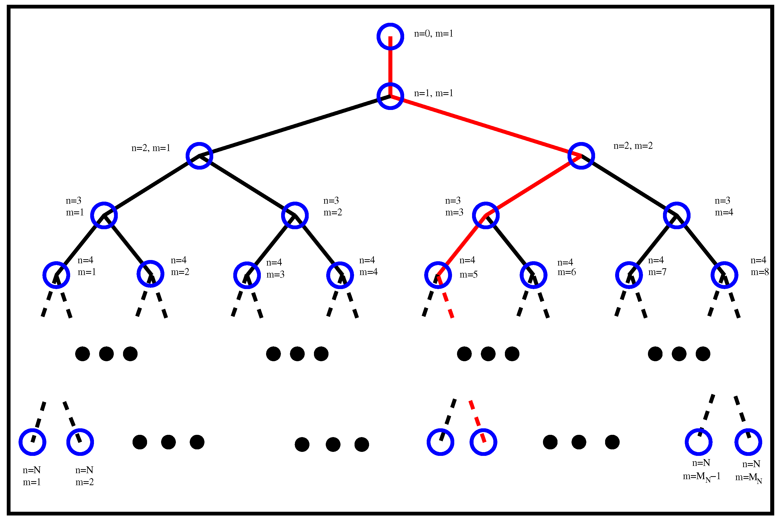
In the spirit discussed in the first paragraph, we here construct and study a binary tree shell model for turbulence that displays intermittency. In this model, energy at each scale is split between multiple different structures. Each structure transfers its energy into two smaller-scale structures, building a binary tree structure as shown in Figure 1. In this way, the number of structures increases exponentially as smaller scales are reached. Such models with binary structure were introduced in the 1990s but have not been investigated extensively [39,40,41]. Here, we follow a similar analysis as in [42], where stationary solutions of non-binary shell models were investigated. We demonstrate that such analysis allows the construction of exact stationary solutions that display intermittency.

2. Multi-Branch Shell Models

We consider the evolution of a turbulent flow modeled by the real amplitudes $U_{n,m}$ of structures of scale ${\ell }_n=1/k_n$ where

$$k_n={\lambda }^n{k}_0\mathrm{or}{\ell }_n={\ell }_0/{\lambda }^n$$

(1)

and $1<\lambda$. At scale ${\ell }_1$, there is one structure whose amplitude is given by $U_{1,1}$; this structure will transfer its energy to $\mu \in \mathbb{N}$ structures of scale ${\ell }_2$, each one of which will transfer its energy to $\mu$ structures of scale ${\ell }_3$ and so on, as shown in Figure 1 for $\mu =2$. The volume of each structure is given by $V_i={\ell }_n^D$, where D is the spatial dimension. If the cascade process is space-filling, the number of substructures $\mu$ is related to $\lambda$ and D by

$${\lambda }^D=\mu .$$

(2)

Accordingly, at energy scale ${\ell }_i$, we have $M_n={\mu }^{n-1}$ (with $M_0=1$) structures so that if we consider N such scales we have a total of

$$Z=1+\sum _{n=1}^N{M}_n=\frac{{\mu }^N-1}{\mu -1}+1$$

(3)

structures. The energy of every structure is given by

$$E_{n,m}=\frac{1}{2}\rho U_{n,m}^2{V}_n=\frac{1}{2}\rho U_{n,m}^2{\ell }_n^D$$

(4)

so the total energy is given by

$$E=\frac{1}{2}\sum _{n=0}^N\frac{1}{M_n}\sum _{m=1}^{M_n}{U}_{n,m}^2$$

(5)

where $\rho$ is from now on taken to be unity.

In the Desnianskii and Novikov model [23], structures of scale ${\ell }_n$ interact with only structures of scale ${\ell }_{n+1}$ and ${\ell }_{n-1}$, and there is no branching $\mu =1$. The amplitudes $U_n$ then follow the following dynamical equation:

$${\dot{U}}_n=a{k}_n[U_{n-1}{U}_{n-1}-\lambda U_n{U}_{n+1}]+b{k}_n[U_n{U}_{n-1}-\lambda U_{n+1}{U}_{n+1}]-\nu k^2{U}_n+F_n$$

(6)

For $\nu =0$ and $F_n=0$, this system conserves the energy (5) (with $M_n=1$) for any value of $a,b$. The flux of energy across a scale ${\ell }_n$ is given by:

$$\begin{array}{ccc}\hfill {\Pi }_n& =& a{k}_n{U}_n{U}_{n-1}{U}_{n-1}+b{k}_n{U}_n{U}_n{U}_{n-1}.\hfill \end{array}$$

(7)

The Desnianskii and Novikov model [23] is the simplest energy-conserving model one can consider. Since its construction, more complex models have been designed that include more distant mode couplings and complex amplitude modes. The newer models display chaotic dynamics and also conserve more invariants than just the energy. The most popular ones are the SABRA and the GUY model [24,25,26,36]. A comparison of the two can be found in [34]. Although these models are more realistic, here, we are going to keep the structure of the Desnianskii and Novikov model [23] because its simplicity allows for analytical treatment.

Expanding on the Desnianskii and Novikov model, allowing each structure to branch out to two ($\mu =2$) smaller-scale structures $U_{n,m}$ results in the following dynamical equation:

$$\begin{array}{ccc}\hfill {\dot{U}}_{n,m}& =& a{k}_n\left[U_{n-1,m^{*}}{U}_{n-1,m^{*}}-\frac{\lambda }{2}\left(U_{n,m}{U}_{n+1,m^{\prime }}+U_{n,m}{U}_{n+1,m^{\prime }+1}\right)\right]+\hfill \\ & & b{k}_n\left[U_{n,m}{U}_{n-1,m^{*}}-\frac{\lambda }{2}\left(U_{n+1,m^{\prime }}{U}_{n+1,m^{\prime }}+U_{n+1,m^{\prime }+1}{U}_{n+1,m^{\prime }+1}\right)\right]\hfill \\ & & -\nu k_n^2{U}_{n,m}+F_{n,m}\hfill \end{array}$$

(8)

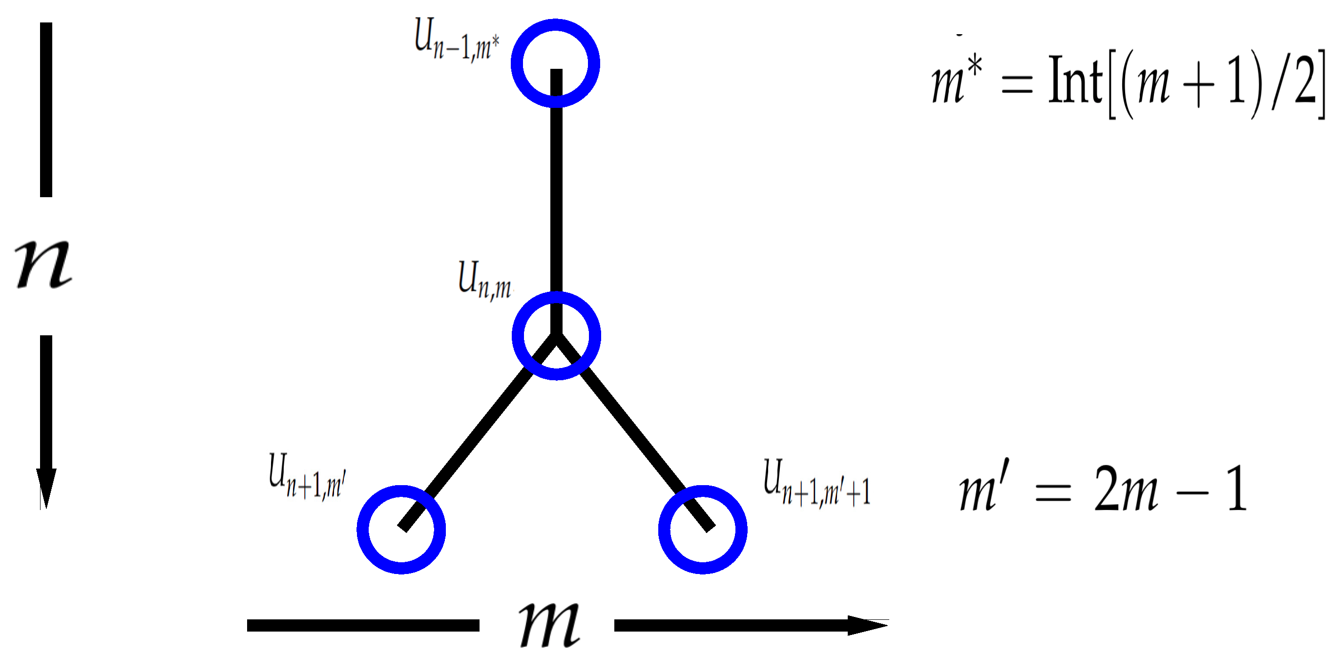
where $\nu$ is the viscosity, $F_{n,m}$ is the forcing, and $a,b$ are again free parameters. The branching diagram for the model given in (9) is provided in Figure 1. The integers $m^{\prime }$ and $m^{\prime }+1$ correspond to the index of scales ${\ell }_{n+1}$, with which the mode $U_{n,m}$ is linked where $m^{\prime }$ is explicitly given by $m^{\prime }=2m-1$ and $m^{*}$ corresponds to the index of scale ${\ell }_{n-1}$ linked to $U_{n,m}$ given by $m^{*}=\mathrm{Int}[(m+1)/2]$, as illustrated in the left panel of Figure 2. For $\nu =0$, $F_{n,m}=0$, and, for any value of $a,b$, the system conserves the energy (5), where now $M_n=2^{n-1}$. The energy flux ${\Pi }_{n,m}$ through a scale ${\ell }_n$ and structure ($n,m$) expressing the rate energy from the large scales ($i<n$) is lost to the smaller scales ($i\ge n$) through the structure m due to the non-linearity, which is given by

$$\begin{array}{ccc}\hfill {\Pi }_{n,m}& =& a{k}_n{U}_{n,m}{U}_{n-1,m^{*}}{U}_{n-1,m^{*}}+b{k}_n{U}_{n,m}{U}_{n,m}{U}_{n-1,m^{*}}\hfill \end{array}$$

(9)

The total flux through scale ${\ell }_n$ is then given by

$${\Pi }_n=\frac{1}{M_n}\sum _{m=1}^{M_n}{\Pi }_{n,m}$$

(10)

Conservation of energy by the non-linear terms implies that, at scales smaller than the forcing scale and larger than the dissipation scale (${\ell }_{\nu }$), the flux ${\Pi }_n$ is constant and equal to the energy injection/dissipation $ϵ$

$${\Pi }_n=ϵ,1<n\ll n_{\nu }$$

(11)

where ${\ell }_{\nu }={({\nu }^3/ϵ)}^{1/4}$ and $n_{\nu }={log}_{\lambda }({\ell }_1/{\ell }_{\nu }).$

The range $1<n\ll n_{\nu }$, where forcing and viscous effects can be neglected, is called the inertial range.

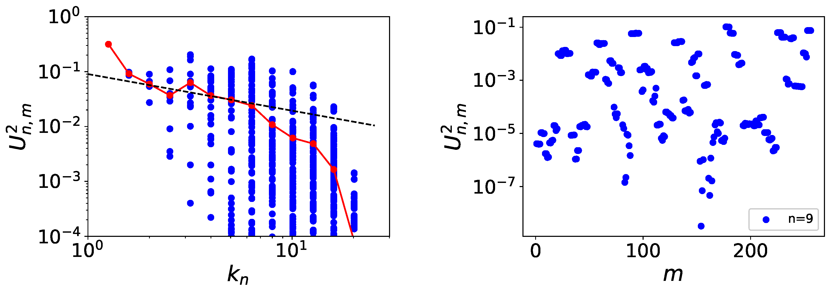
In Figure 3, we plot the energy spectra $U_{n,m}^2$ as a function of n with blue dots, while the red dots indicate the averaged value $\overline{U_n^2}=\left({\sum }_m{U}_{n,m}^2\right)/M_n$ from a realisation of a simulation of Equation (9) performed with $N=14,\lambda =2^{1/3}$ forced at $n=1$, while the amplitude of the mode $n=0$ was kept fixed at $U_{0,1}=0$. The forcing for this simulation was constant in time and random initial conditions were used. The spectra were calculated a few turnover times after the initialization. At that time, the amplitudes $U_{n,m}$ appear to be very dispersed even for the same value of n. The averaged value follows power law close to the Kolmogorov scaling $\overline{U_n^2}\propto k_n^{-2/3}$, although individual $U_{n,m}^2$ can vary orders of magnitude from this mean value. This indicates that higher-order statistics can deviate from the dimensional analysis spectrum. If the simulation is carried over to longer times, there is a slow synchronisation between same n modes for large n such that $U_{n,m}$ attain similar values for all m. This effect is due to viscosity and has been noted in previous works [40,41] and is referred to as phase synchronisation. It can be avoided if additional interaction terms between same n modes are added. Here, we do not add this further complexity and consider only interactions as depicted in Figure 2 and focus only on the inertial properties.

The present model is computationally expensive as its complexity increases as $2^N$. As a result, it is not easy to obtain a long inertial range (large N) to investigate the resulting power-law behaviours numerically. On the other hand, its simplicity allows for analytical treatment, which is what we are examining in the next section by constructing exact inertial range solutions of arbitrary large n.

3. Inertial Range Intermittent Solutions

We look for stationary solutions of Equation (9) in the inertial range where forcing and dissipation can be ignored. Stationarity implies that, for any $n,m$:

$$\begin{array}{ccc}\hfill 0& =& a\left[U_{n-1,m^{*}}{U}_{n-1,m^{*}}-\frac{\lambda }{2}\left(U_{n,m}{U}_{n+1,m^{\prime }}+U_{n,n}{U}_{n+1,m^{\prime }+1}\right)\right]\hfill \\ & +& b\left[U_{n,m}{U}_{n-1,m^{*}}-\frac{\lambda }{2}\left(U_{n+1,m^{\prime }}{U}_{n+1,m^{\prime }}+U_{n+1,m^{\prime }+1}{U}_{n+1,m^{\prime }+1}\right)\right]\hfill \end{array}$$

(12)

The way we proceed to find such a solution is the following: given $U_{n-1,m^{*}}$ and $U_{n,m}$, we look for $U_{n+1,m^{\prime }}$ and $U_{n+1,m^{\prime }+1}$ such that the equation above is satisfied; then, we proceed to the next scale and search for $U_{n+2,2m^{\prime }-1}$ and $U_{n+2,2m^{\prime }}$ and so on, finding a recursive relation that provides all $U_{n,m}$. The solutions only depend on the relative amplitude of $U_{n,m}$, so we define their normalised ratio as

$$r_{n,m}=\frac{U_{n,m}{\lambda }^{1/3}}{U_{n-1,m^{*}}}$$

(13)

To simplify the notation, we denote

$$r=r_{n,m},x=r_{n+1,m^{\prime }}y=r_{n+1,m^{\prime }+1}\mathrm{and}b=c{\lambda }^{1/3}$$

(14)

and then stationary solutions of (12) satisfy

$$\begin{array}{ccc}\hfill 0& =& U_{n,m}^2{\lambda }^{2/3}\left(a\left[\frac{1}{r^2}-\frac{1}{2}\left(x+y\right)\right]+c\left[\frac{1}{r}-\frac{1}{2}\left(x^2+y^2\right)\right]\right)\hfill \end{array}$$

(15)

which simplifies to

$$\begin{array}{c}\hfill {\left(x+\frac{a}{2c}\right)}^2+{\left(y+\frac{a}{2c}\right)}^2=2\left(\frac{a}{c{r}^2}+\frac{1}{r}+\frac{a^2}{4c^2}\right).\end{array}$$

(16)

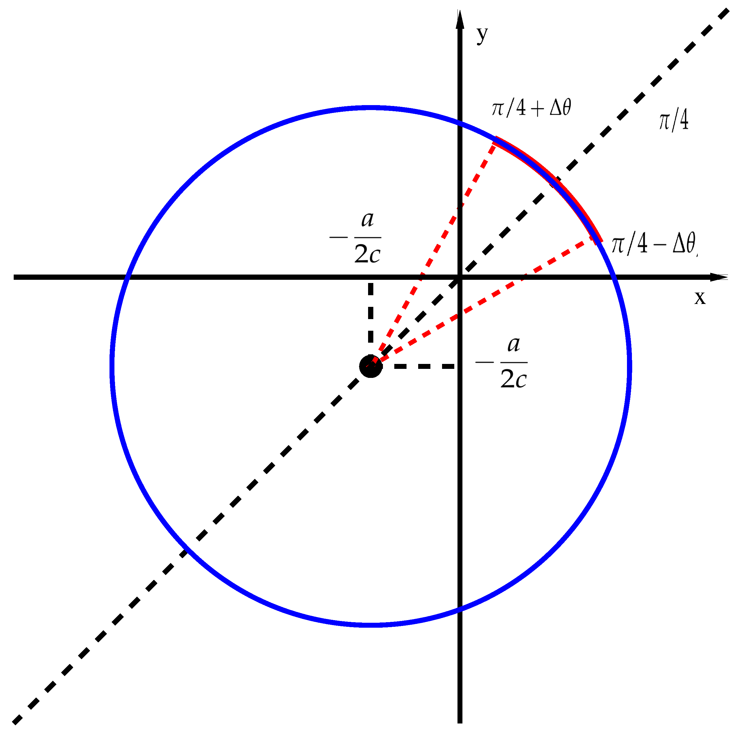
which has real solutions only if

$$\begin{array}{c}\hfill 0\le \frac{a}{c{r}^2}+\frac{1}{r}+\frac{a^2}{4c^2}=R^2.\end{array}$$

(17)

The solutions $(x,y)$ form a circle in the $x,y$ plane centered at $(-a/2c,-a/2c)$ and with radius R depicted in the right panel of Figure 4. It is important to note that any point $(x,y)$ in this circle is a solution of (16), and thus we have multiple possible solutions. The condition (17) is satisfied for positive $r,a,c$, which will be the focus of the present investigation. Returning to the $r_{n,m}$ notation, the values of $r_{n+1,m^{\prime }}$ and $r_{n+1,m^{\prime }+1}$ that satisfy the stationarity condition can be written in full generality as

$$\begin{array}{ccc}\hfill r_{n+1,m^{\prime }}& =& -\frac{a}{2c}+\sqrt{2}cos\left({\theta }_{n,m}\right)\sqrt{\frac{a}{c{r}_{n,m}^2}+\frac{1}{r_{n,m}}+\frac{a^2}{4c^2}}\hfill \end{array}$$

(18)

$$\begin{array}{ccc}\hfill r_{n+1,m^{\prime }+1}& =& -\frac{a}{2c}+\sqrt{2}sin\left({\theta }_{n,m}\right)\sqrt{\frac{a}{c{r}_{n,m}^2}+\frac{1}{r_{n,m}}+\frac{a^2}{4c^2}}\hfill \end{array}$$

(19)

where ${\theta }_{n,m}$ is arbitrary. Equations (18) and (19) form a recurrence relation out of which, given $r_{1,1}$ and a choice of ${\theta }_{n,m}$, one can construct all $r_{n,m}$. Then, given $r_{n,m}$, one can obtain $U_{n,m}$ based on (14) as

$$U_{n,m}=U_{1,1}{r}_{1,1}{r}_{2,m_1}{r}_{3,m_2}\cdots r_{n,m}$$

(20)

where $m_1,m_2,\cdots$ are the m one crosses along the path from (1,1) to ($n,m$) as shown by the red line in Figure 1. This recurrence relation, however, does not always lead to bounded solutions of $r_{n,m}$. For some values of ${\theta }_{n,m}$, the resulting $x,y$ can be negative or zero. Negative values can lead to un-physical solutions with negative flux from the small to the large scales. If the flux ${\Pi }_{n,m}$ is negative for some (n,m), then the sum of the flux of the “daughter” nodes ${\Pi }_{n+1,m^{\prime }}+{\Pi }_{n+1,m^{\prime }+1}$ has to be negative and equal to ${\Pi }_{n,m}$ and so on for their “daughter” nodes. There would then exist at least one descendant at each scale with negative flux, and this can only be realised if there is a source of energy at the very small scales, which is un-physical. Negative flux stationary solutions are thus not accepted. Furthermore, if x or y is zero, it means that the particular branch is zero for all subsequent values (i.e., all descendants). We need thus to limit the choice of $\theta$ so that positive and finite $r_{n,m}$ are obtained.

The simplest case is obtained by choosing ${\theta }_{n,m}=\pi /4$. It corresponds to an equal part of energy being distributed to the left and the right branch and leads to the Kolmogorov solution $r_{n,m}=1$ or in terms of the velocity $U_{n,m}={\lambda }^{n/3}$) (where $U_{1,1}=1$ is assumed). It corresponds to a finite flux non-intermittent (self-similar) solution.

Intermittency, however, can manifest itself if we chose ${\theta }_{n,m}\ne \pi /4$ so that energy is not equally distributed in the left and right branch. Here, we will chose ${\theta }_{n,m}$ randomly with uniform distribution in the range ${\theta }_{min}=\pi /4-\Delta \theta <{\theta }_{n,m}<\pi /4+\Delta \theta ={\theta }_{max}$ for a given $\Delta \theta <\pi /4$, as shown in red in Figure 4. Then, it can be shown that, for $c>a$, there exists $r_{max}>r_{min}>0$ such that, for all $r\in (r_{max},r_{min})$, both $x\in (r_{max},r_{min})$ and $y\in (r_{max},r_{min})$. For $c\le a$, the recurrence relation converges either to $r_{n,m}=0$ or $r_{n,m}=\infty$ and we are going to limit ourselves only to the $c>a$ case here. To obtain $r_{max},r_{min}$, one needs to note that, from the recurrence relation (19), the largest value of $r_{n+1,m^{\prime }}=r_{max}$ is obtained when $\theta ={\theta }_{max}$ and $r_{n,m}=r_{min}$, while the smallest value of $r_{n+1,m^{\prime }}=r_{min}$ is obtained when $\theta ={\theta }_{min}$ and $r_{n,m}=r_{max}$. This leads to the following relations

$$\begin{array}{ccc}\hfill r_{max}& =& -\frac{a}{2c}+\sqrt{2}cos\left({\theta }_{min}\right)\sqrt{\frac{a}{c{r}_{min}^2}+\frac{1}{r_{min}}+\frac{a^2}{4c^2}}\hfill \end{array}$$

(21)

$$\begin{array}{ccc}\hfill r_{min}& =& -\frac{a}{2c}+\sqrt{2}cos\left({\theta }_{max}\right)\sqrt{\frac{a}{c{r}_{max}^2}+\frac{1}{r_{max}}+\frac{a^2}{4c^2}}.\hfill \end{array}$$

(22)

We arrive at exactly the same relations if we examine Equation (19).

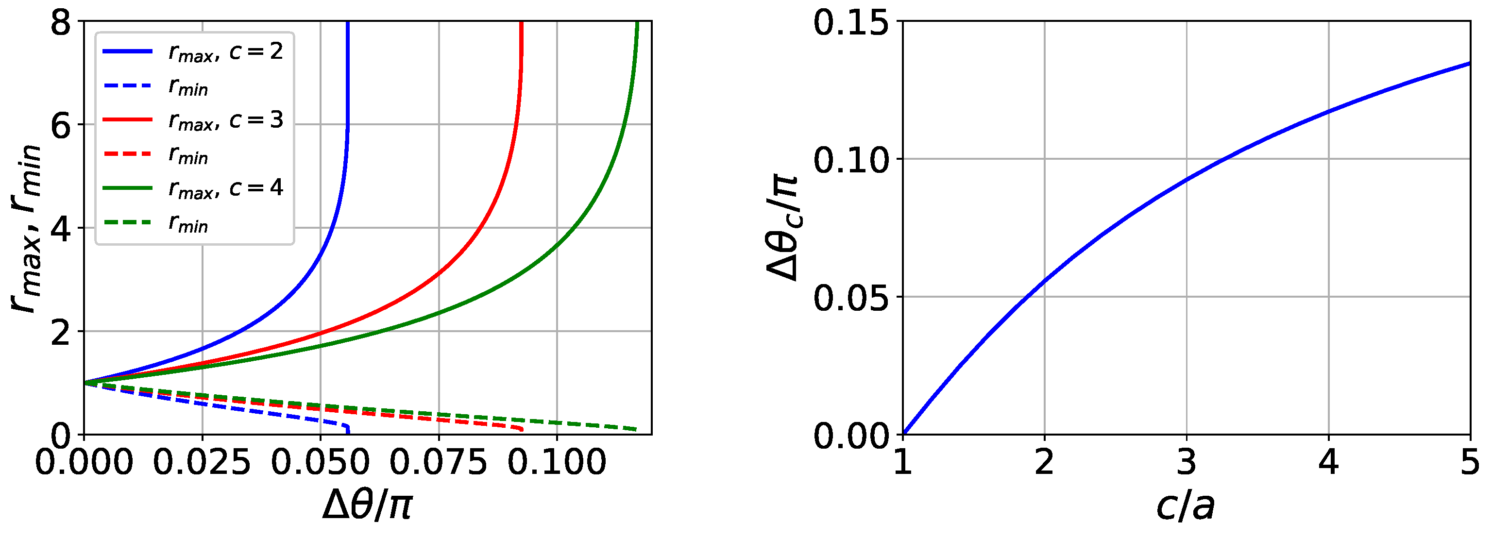
We solved Equations (21) and (22) numerically and the results are shown in the left panel of Figure 5 for three different values of $c/a$. For $\Delta \theta =0$, only the Kolmogorov solution is allowed with $r_{max}=r_{min}=1$. As $\Delta \theta =0$ increases, $r_{n,m}$ cover a wider range of values up until a critical value of $\Delta \theta =\Delta {\theta }_c$ for which $r_{min}$ becomes zero and $r_{max}$ diverges. The value of this critical angle as a function $c/a$ is shown in the right panel of the same figure. $\Delta {\theta }_c$ is zero for $c/a=1$ and grows for larger values approaching $\Delta {\theta }_c=\pi /4$ as $c/a\to \infty$ (not demonstrated here).

For any given choice of $\Delta \theta <\Delta {\theta }_c$, we can construct an ensemble of exact solutions of the present model by following the recurrence relations (18) and (19), picking each time randomnly ${\theta }_{n,m}\in (\pi /4-\Delta \theta ,\pi /4+\Delta \theta )$ and reconstructing $U_{n,m}$ by Equation (20). We note that, other than $c/a$, the only other parameter that controls the ensemble of solutions considered is $\Delta \theta /\Delta {\theta }_c$, which provides a measure of how much our ensemble deviates from the Kolmogorov solution $\Delta \theta =0$. This process has direct links with the random cascade models studied in the past [43,44,45]; however, we need to note that, unlike the random cascade models, the solutions found here are energy-conserving.

4. Statistical Behaviour and Intermittency

In this section, we examine a large ensemble of the exact solutions shown in the previous section and investigate their properties. For our investigation, we have set $c/a=2$ and we consider only a single path (as the one shown in red in Figure 1) and not the full tree. The differences in the statistics between the two choices (single path and full tree) lie in the cross correlations between different modes that are not captured in the single path. As an example, we mention that the flux ${\Pi }_n$ in Equation (10) is identically equal to $ϵ$ for every realisation, while the flux ${\Pi }_{n,m}$ given in Equation (9) fluctuates and only its mean value is equal to $ϵ$

$$\langle {\Pi }_{n,m}\rangle ={\Pi }_n=ϵ.$$

Along such path, we consider three different ensembles for $\Delta \theta /\Delta {\theta }_c=0.1,0.5,0.9$, each one composed of ${10}^7$ different solutions. The solutions were constructed by picking randomly ${\theta }_{n,m}$ for each node examined, from a uniform distribution between $\pi /4-\Delta \theta$ and $\pi /4+\Delta \theta$. The value of n varied from $n=1$ to $n=200$. We note that, if the full tree was investigated instead of a single path for such large value n, it would require to solve for $2^{200}$ degrees of freedom, which is computationally unattainable.

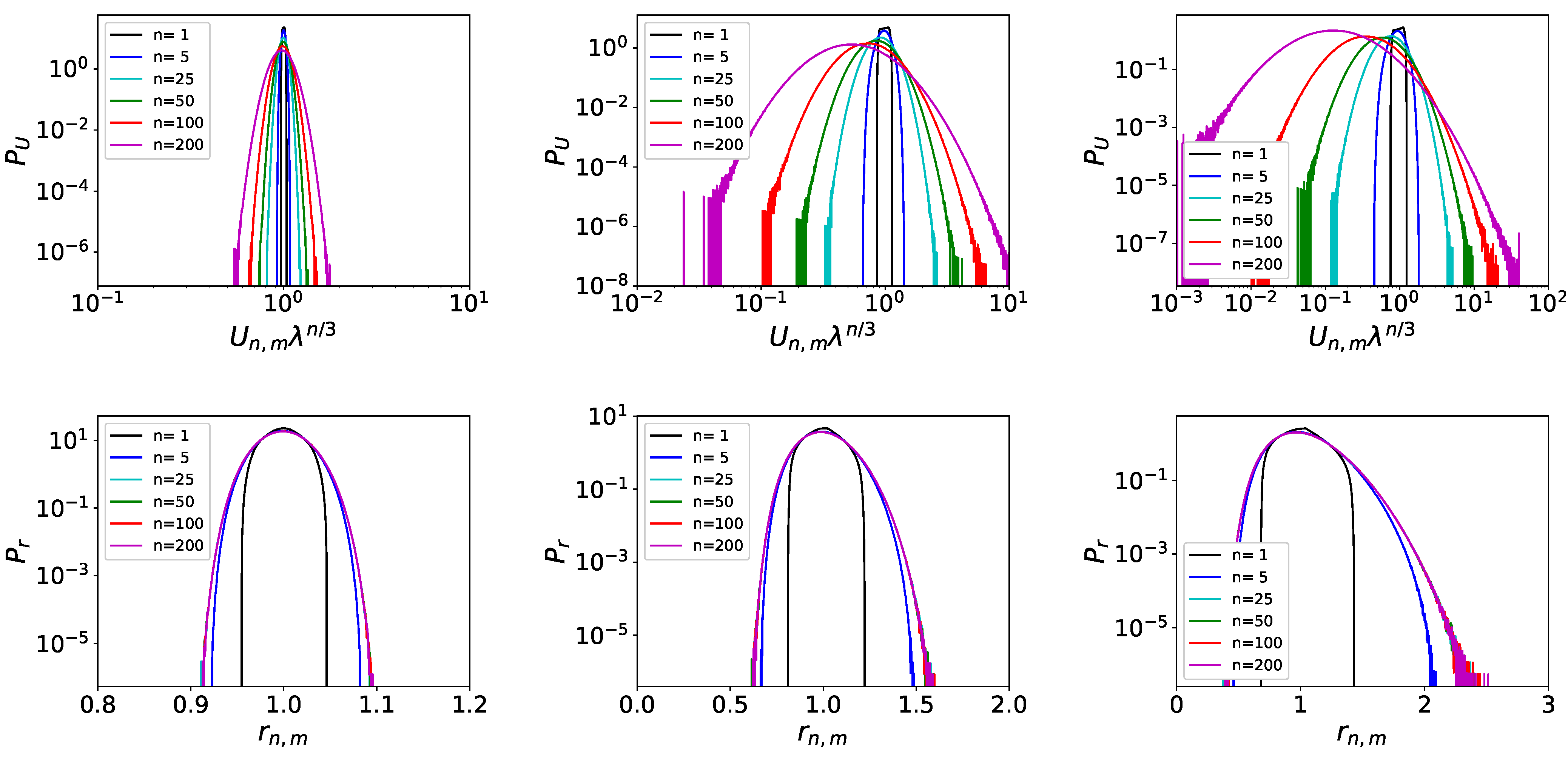
In the top panels of Figure 6, we plot the probability distribution function (PDF) $P_U\left(U_{n,m}\right)$ of the variable $U_{n,m}$ for the three values of $\Delta \theta /\Delta {\theta }_c=0.1,0.5,0.9$ (from left to right) and different values of n. The PDFs of different values of n do not seem to overlap, although the x-axis has been normalised by the Kolmogorov prediction ${\lambda }^{-1/3}$. Instead, as large values of n are reached, the PDFs display larger tails, reaching values of $U_{n,m}$ much larger and much smaller than their mean values. The closer $\Delta \theta$ is to the critical value $\Delta {\theta }_c$, the larger this deviation is. On the other hand, the PDFs $P_r\left(r_{n,m}\right)$ of the ratios $r_{n,m}$ that are displayed in the lower panels of Figure 6 do not display such widening. For sufficiently large n, all PDFs collapse to the same functional form that depends only on the choice of $\Delta {\theta }_c$. This implies that, while $U_{n,m}$ are not self-similar under scale transformations, their ratios $r_{n,m}$ are!

The same behaviour can be observed for the energy fluxes ${\Pi }_{n,m}$. In the top panels of Figure 7, we plot the PDFs $P_{\Pi }$ of ${\Pi }_{n,m}$ for the same values of $\Delta \theta$ and n as in Figure 6. As with the velocity amplitudes $U_{n,m}$, as n is increased, the PDFs of ${\Pi }_{n,m}$ widen without collapsing to an n-independent form. In the lower panel of the same figure, we plot the the PDFs $P_{\pi }\left({\pi }_{n,m}\right)$ of the flux ratio ${\pi }_{n,m}$. It is defined as

$${\pi }_{n,m}=\frac{{\Pi }_{n,m}}{{\Pi }_{n-1,m^{*}}}$$

(23)

after a little algebra and using (9) and (18) leads to

$${\pi }_{n+1,m^{\prime }}=1+f\left(r_{n,m}\right)cos\left(2{\theta }_{n,m}\right)$$

(24)

where $f\left(r\right)=1+{(a/2c)}^2{r}^2/(a/c+r)$. The flux ratio, much like the velocity ratio $r_{n,m}$, does converge to an n-independent PDF as large values of n are reached. Furthermore, the functional form of this PDF appears to be flat, limited by a minimum and a maximum value of ${\pi }_{n,m}$. This appears to be so because $f\left(r\right)$ in (24) varies little with r for small variations in r and the variations in ${\pi }_{n,m}$ are mostly controlled by the variations in ${\theta }_{n,m}$.

Given that the PDFs of $r_{n,m}$ and ${\pi }_{n,m}$ arrive at an n-independent form, a large n has some implications for the evolution in n of the PDFs $P_U,P_{\Pi }$. Both $U_{n,m}$ and ${\Pi }_{n,m}$ can be written as a product of all $r_{n^{\prime },m}$ and ${\pi }_{n^{\prime },m}$ with $n^{\prime }\le n$. As a result, the logarithms of $U_{n,m}$ and ${\Pi }_{n,m}$ can be written as

$$ln\left(U_{n,m}\right)=ln\left(U_{1,1}\right)+n{L}_U,ln\left({\Pi }_{n,m}\right)=ln\left({\Pi }_{1,1}\right)+n{L}_{\Pi }$$

(25)

where $L_U$ and $L_{\Pi }$ stand for the mean value of the logarithms of $r_{n,m}$ and ${\pi }_{n,m}$, respectively:

$$L_U=\frac{1}{n}\sum _{n^{\prime }=1}^{n}ln\left(r_{n^{\prime },m}\right),\mathrm{and}{L}_{\Pi }=\frac{1}{n}\sum _{n^{\prime }=1}^{n}ln\left({\pi }_{n^{\prime },m}\right).$$

(26)

The properties of $U_{n,m}$ and ${\Pi }_{n,m}$ remind of the random cascades studied in the past [43,44,45]. However, while the random cascade models were not conserving energy, in the present model, energy is conserved exactly. Another important difference here is that $r_{n^{\prime },m}$ and ${\pi }_{n,m}$ are not independent but each one depends on the value of the previous one. Nonetheless, we can proceed assuming such independence, although not entirely correct. In that case, $P_U$ and $P_{\Pi }$ can be reconstructed using large deviation theory [46]. In this framework, $L_U$ and $L_{\Pi }$ follow for large n a distribution of the form

$$P_{L_U}\left(L_U\right)\propto exp[-n{I}_U\left(L_U\right)],\mathrm{and}{P}_{L_{\Pi }}\left(L_{\Pi }\right)\propto exp[-n{I}_{\Pi }\left(L_{\Pi }\right)]$$

(27)

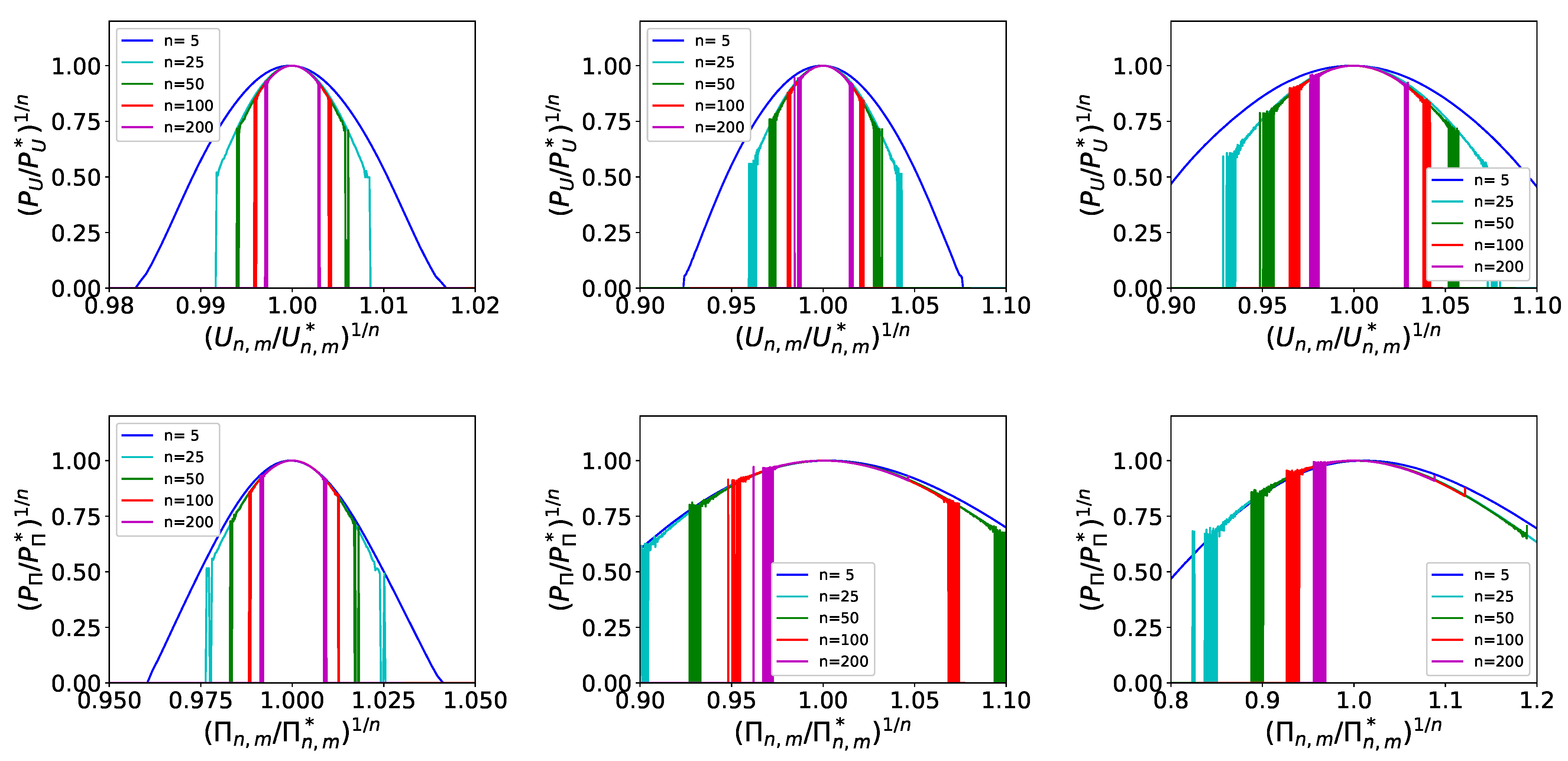
where $I_U$ and $I_{\Pi }$ are called the rate functions that can in principle be obtained from $P_r$ and $P_{\pi }$ using the Legendre–Fenchel transform [46]. Here, we limit ourselves in noting that, if $P_{L_U}$ and $P_{L_{\Pi }}$ follow the form of Equation (27), then the distributions of $U_{n,m}$ and ${\Pi }_{n,m}$ that are linked to $L_U$ and $L_{\Pi }$ by (25) should take the form

$$P_U\left(U_{n,m}\right)\propto exp\left[-n{I}_U\left(\frac{1}{n}ln\left(\frac{U_{n,m}}{U_{1,1}}\right)\right)\right],P_{\Pi }\left({\Pi }_{n,m}\right)\propto exp\left[-n{I}_{\Pi }\left(\frac{1}{n}ln\left(\frac{{\Pi }_{n,m}}{{\Pi }_{1,1}}\right)\right)\right]$$

(28)

where only the largest terms in n are kept. To test this prediction, we plot in Figure 8 ${(P_U/P_U^{*})}^{1/n}$ as a function ${(U_{n,m}/U^{*})}^{1/n}$ (top panels) and ${(P_{\Pi }/P_{\Pi }^{*})}^{1/n}$ as a function ${({\Pi }_{n,m}/{\Pi }^{*})}^{1/n}$, where $U^{*}$ and ${\Pi }^{*}$ correspond to the value at which the probability obtains its maximum $P_U^{*},P_{\Pi }^{*}$. With this normalization, the PDFs both for $U_{n,m}$ and for ${\Pi }_{n,m}$ collapse, indicating that the large deviation principle works well for this model.

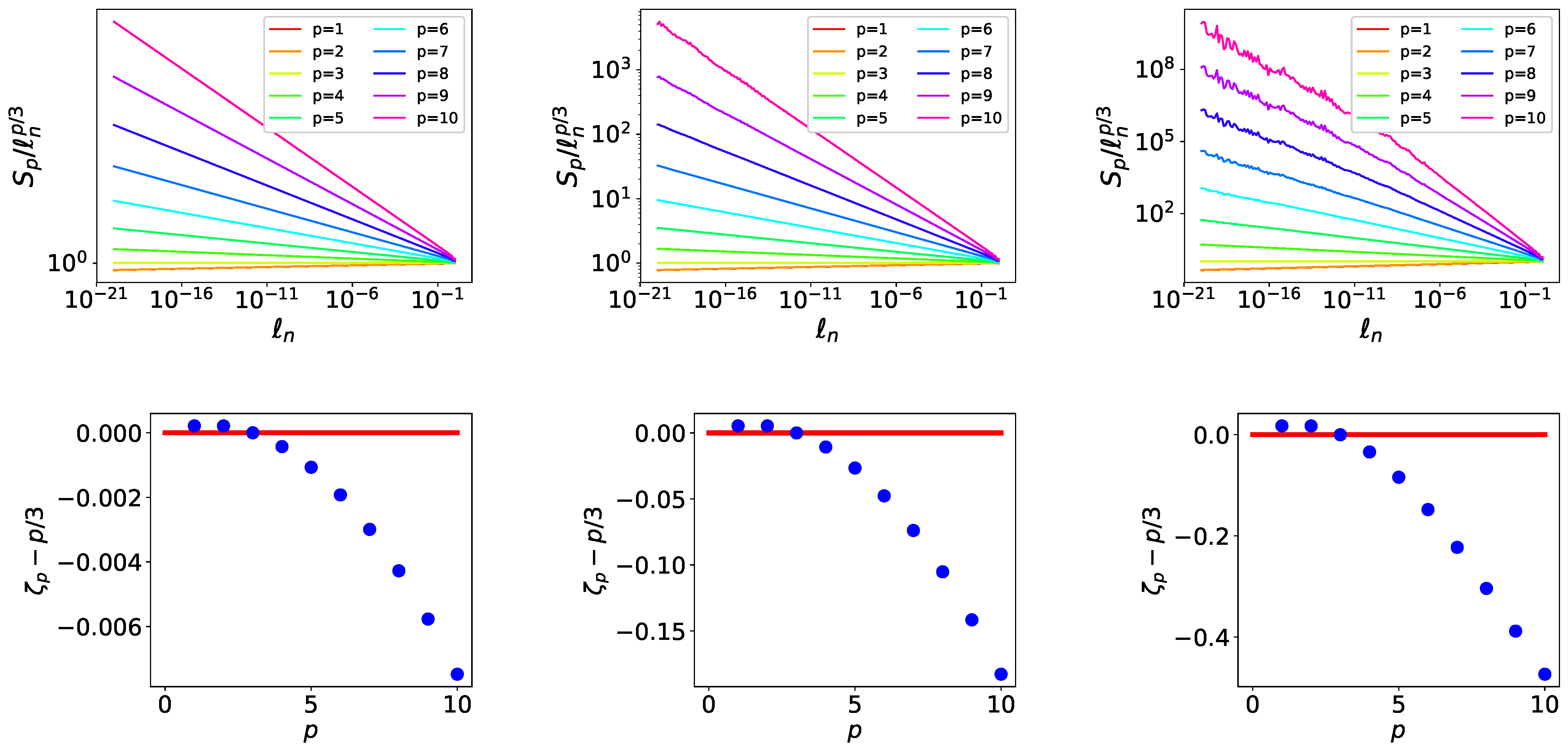
As a final look at the intermittency problem, we display in the top panels of Figure 9 the first ten structure functions $S_p\left({\ell }_p\right)$ defined as

$$S_p\left({\ell }_n\right)=〈U_{n,m}^p〉$$

(29)

where the angular brackets stand for ensemble average. The structure functions have been normalised by the Kolmogorov scaling to emphasise the differences. The structure functions are fitted to power laws

$$S_p\left({\ell }_n\right)\propto {\ell }_n^{{\zeta }_p}$$

(30)

and the measured exponents ${\zeta }_p$ are plotted in the lower panels of Figure 9. The exponents show similar behaviour, with real turbulence displaying larger values for $p<3$ and smaller values for $p>3$, while the exact result ${\zeta }_3=1$ is satisfied. It is worth noting that the deviations from the Kolmogorov scaling are not universal but depend on our choice of ensemble, which is controlled by $\Delta \theta$.

5. Discussion and Conclusions

One can argue that the exact stationary solutions obtained in this work have little to do with real turbulence that displays chaotic spatio-temporal dynamics. This may be true and multi-branch models with two neighbour interactions as in [39,40,41] that display chaotic dynamics should be investigated instead. The present results, however, do point to a clear instructive demonstration of how intermittency can appear in realistic flows and how it can be modeled. Furthermore, it leads to a series of clear messages that are described below that are of great use in future turbulence research and can guide measurements in numerical simulations and experiments.

First, we note that intermittency appearing in stationary fields found here comes in contrast with the typical shell model studies in single-branch models for which intermittency comes from the temporal dynamics alone as only a single structure exists for each scale ${\ell }_n$. In the latter case, intermittency has been linked to the temporal dynamics through the fluctuation dissipation theorem [37]. In reality, both temporal and spatial dynamics contribute to the presence of intermittency and their role needs to be clarified.

In the present model, randomness comes from our choice of ${\theta }_{n,m}$ and the resulting intermittency depends on that choice. In reality (or in more complex shell models), such randomness comes from local chaotic dynamics that need to studied in order to clarify which processes lead to enhanced cascade and with what probability. Multi-branch models based on the more complex GOY or SABRA as proposed in [39,40,41] can help in this direction. The additional coupling terms introduced in these works avoid phase synchronization and lead to chaotic dynamics. Chaos can remove the arbitrariness of the choice of $\theta$ that should ideally be self-imposed by the dynamics.

Perhaps the most interesting implication of this work is that it suggests new ways to plot data from experimental and numerical simulations. One way suggested by this work is, instead of focusing on the PDFs of velocity differences, experimental or numerical data could focus on the PDFs of ratios of velocity differences. The latter are shown in this work to become scale-independent and could lead to more precise measurements. An alternative way is to re-scale the PDFs of velocity differences using the large deviation prediction (27), as was conducted in Figure 8. Of course, realistic data $n\propto ln(L/{\ell }_n)$ are not precisely defined and an optimal choice should be searched for.

A good model of a complex phenomenon, in the authors’ opinion, is not one that quantitatively reproduces experimental measurements through parameter fitting but rather one that unravels the processes involved. In that respect, we believe that the present model and results are very fruitful. We only hope that this work comes close to the standards set by Jack Herring. A.A. met Jack Herring during his ASP post doc in 2004–2006. Jack is fondly remembered stopping by the offices of post docs just to see if they are OK. He will be greatly missed.