The Surprising Roles of Turbulence in Tropical Cyclone Physics

Abstract

Tropical cyclones have long been known to be powered by turbulent enthalpy fluxes from the ocean’s surface and slowed by turbulent momentum fluxes into the surface. Here, we review evidence that the development and structure of these storms are also partially controlled by turbulence in the outflow near the storm’s top. Finally, we present new research that shows that tropical cyclone-like, low-aspect-ratio vortices are most likely in systems in which the bottom heat flux is controlled by mechanical turbulence, and the top boundary is insulating.

1. Introduction

Some 90 tropical cyclones develop globally each year, producing among the strongest winds and storm tides of any atmospheric phenomenon. Here, we review the critical, multiple roles that turbulence plays in tropical cyclone physics. We dedicate this paper to the memory of Jack Herring, whose own work on turbulence inspired parts of what we present here.

Tropical cyclones are driven by turbulent enthalpy fluxes from the ocean, as shown long ago by Riehl [1] and Kleinschmidt [2]. More recently, numerical simulations of dry tropical cyclones demonstrated that phase change of water is not necessary, though it does affect the structure and intensity of the vortices [3,4,5,6]. In the real-world moist case, most of the turbulent enthalpy flux is in the form of latent heat, and so the air–sea temperature differential is small. This, coupled with very strong surface winds, implies that the turbulence driving the surface fluxes is almost entirely mechanical. Likewise, the power dissipation at the sea’s surface increases with the cube of the surface wind speed. An upper bound on the wind speed in a steady, axisymmetric tropical cyclone can be derived by equating the power generated by the thermal cycle of the storm with that dissipated by turbulence; this upper bound has been shown to be an excellent predictor of maximum surface wind speed in numerical simulations [7] and bounds the probability distribution of storm lifetime maximum winds in nature [8]. In Section 2, we review the important role of boundary layer turbulence and the challenge of estimating surface fluxes in the highly perturbed sea states in intense storms.

A complete solution of the equations governing a steady, axisymmetric tropical cyclone demands an upper boundary condition as well as the surface boundary conditions described above. As the outflow is constrained by both rotation and ambient stratification, an appropriate upper boundary condition is not evident from first principles. We argued that the outflow of tropical cyclones is self-stratifying, maintaining a constant, critical Richardson Number [9]. In Section 3, we review this idea and its implications for tropical cyclone structure and intensity and present new field observations supporting the idea of self-stratifying outflow.

Research on geophysical convection and on idealized Rayleigh–Bénard convection has proceeded on largely different paths for many decades, coming to quite different conclusions about the nature of convection. In particular, the Rayleigh–Bénard formalism predicts and laboratory experiments confirm that fluxes from the boundaries continue to depend on molecular diffusivities even in the limit of infinite Rayleigh Number, whereas convective boundary layer theory, supported by field experiments, shows no explicit dependence on molecular diffusivity. In rotating Rayleigh–Bénard convection, the horizontal spacing of vortices scales with the fluid depth, whereas tropical cyclones in idealized experiments are spaced at much greater distances. In Section 4, we show evidence that these discrepancies result from very different assumptions about the physical natures of the horizontal boundaries in the two cases.

2. The Critical Role of Boundary Layer Turbulence in Tropical Cyclone Physics

As air spirals into the core of a mature tropical cyclone, seawater evaporates into it, and turbulent kinetic energy is dissipated into heat. These two processes raise the specific moist entropy of the air, defined as [10]

$$s=\left(c_p+c_l{q}_t\right)\ln \left(T\right)+\frac{L_{v}q}{T}-\left(1+q_t\right)R_d\ln \left(p\right)-R_v{q}_{t}T\ln (H),$$

(1)

where $c_p$ is the heat capacity at constant pressure of dry air, $c_l$ is the heat capacity of liquid water, $q_t$ is the mass concentration of water in all its phases, $T$ is absolute temperature, $q$ is the mass concentration of water vapor, $L_v$ is the latent heat of vaporization, $R_d$ is the universal gas constant divided by the mean molecular weight of dry air, $p$ is total air pressure, $R_v$ is the universal gas constant divided by the molecular weight of water, and H is the relative humidity.

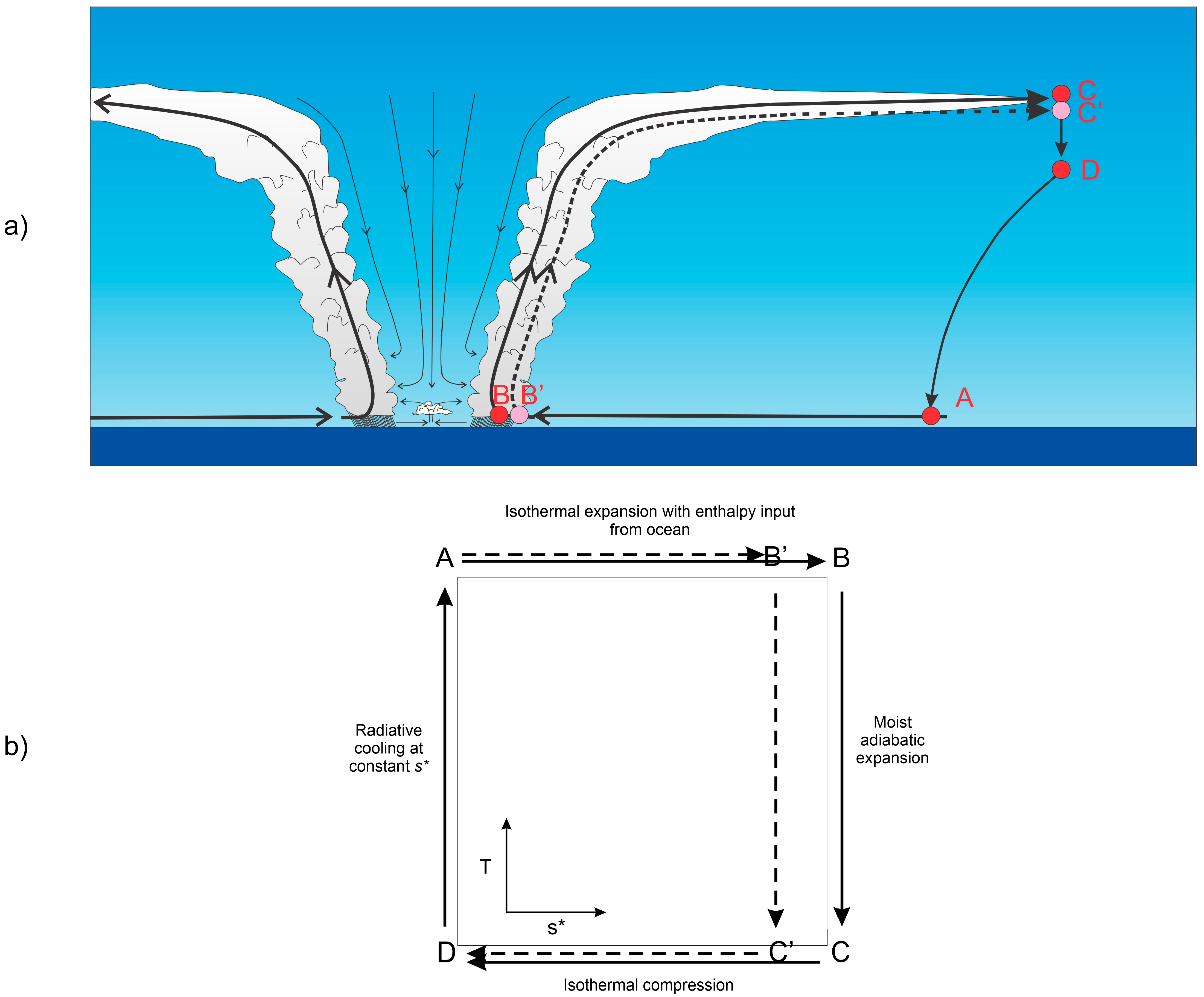
The air arrives in the eyewall with increased entropy and then ascends through the eyewall, conserving its entropy in a nearly adiabatic expansion. The excess entropy is lost at very low temperatures (usually less than −70 °C in the upper troposphere (15–18 km above the surface) through a combination of asymmetric export and infrared radiative cooling. Eventually, air descends back into the boundary layer, following the moist adiabatic temperature profile typical of the unperturbed tropical atmosphere. (Although this air descends unsaturated and is cooled radiatively, it follows the same thermodynamic pathway as a saturated sample, in which evaporation of condensed water takes place. A hurricane in which phases changes of water occur reversibly has been successfully simulated [6]).

These four legs of the airflow can be described as a nearly ideal Carnot cycle [11], with isothermal expansion as air flows along the surface into the low-pressure core while the enormous heat bath provided by the ocean keeps it at nearly constant temperature, followed by moist adiabatic expansion, followed by nearly isothermal compression, and, finally, followed by compression along a moist adiabat.

In Figure 1a, we sketch two adjacent Carnot circuits in the radius–height plane: A-B-C-D-A, and A-B’-C’-D-A. As the gradients near points A and D are very weak, we ignore the differences between the thermal properties of air of the two circuits at these points. These cycles are illustrated in thermodynamic phase space in Figure 1b. The ordinate is absolute temperature, and the abscissa is the entropy of saturated air $s^{\ast }$. In [7], we developed integral relationships for both circuits by combining the first law of thermodynamics with the kinetic energy equation and integrating the result around the circuits. By subtracting one the circuit integral of the first circuit from the second, we arrived at

$${\displaystyle \underset{inner}{\oint }T\frac{ds}{dt}}=-{\displaystyle \underset{inner}{\oint }V·F-{\displaystyle \underset{inner}{\oint }\frac{d{q}_t}{dt}\left[\frac{1}{2}|V{|}^2+gz\right]}},$$

(2)

where “inner” denotes the circuit B’-B-C-C’-B’. The left side of (2) is the total thermodynamic energy available around the circuit, whereas the first term on the right is the power dissipation (dot product of the vector velocity and frictional slowing, $F$). The last term in Equation (2) represents the work used to accelerate the water substance to the free stream velocity and to lift it against gravity $g,$ where $z$ is altitude. This term can be shown to be small [7].

Therefore, Equation (2) may be approximated by

$${\displaystyle \underset{inner}{\oint }T\frac{ds}{dt}}=-{\displaystyle \underset{inner}{\oint }V·F}.$$

(3)

We take points B and B’ to lie on either side of the radius of maximum surface wind speed. We take entropy and angular momentum to be conserved on the legs B-C and B’-C’. Entropy increases from B’ to C’, and the same quantity is lost between C and C’. Angular momentum is diminished from B’ to B, and the same amount is regained by turbulent exchange with the environment between C and C’. However, the right hand side of Equation (3) evaluated between C and C’ is small compared to the contribution along the leg B’-B, provided the point C is not too far from the storm center [11], and we neglect it here. We model the turbulent exchanges between the air and the surface according to the neutral aerodynamic flux formulae. With these assumptions, and taking the path length B’-B to be vanishingly small, Equation (3) becomes

$$\frac{T_s-T_{out}}{T_s}\left[C_{k10}\left|V_{10}\right|\left(k_0^{\ast }-k_{10}\right)+C_{D10}|V_{10}{|}^3\right]=C_{D10}|V_{10}{|}^3,$$

(4)

where $\left|V_{10}\right|$ is the 10 m wind speed at the radius of maximum winds, the drag coefficient $C_{D10}$ and enthalpy exchange coefficient $C_{k10}$ pertain to 10 m altitude, $T_s$ is the surface temperature, $T_{out}$ is the temperature at C-C’, $k_0^{\ast }$ is the saturation enthalpy of the sea surface, and $k_{10}$ is the enthalpy at 10 m. (The altitude 10 m is used here only by convention).

Collecting terms in Equation (4) results in an expression for the 10 m wind speed:

$$|V_{10}{|}^2=\frac{C_{k10}}{C_{D10}}\frac{T_s-T_{out}}{T_{out}}\left(k_0^{\ast }-k_{10}\right).$$

(5)

The surface wind speed calculated this way has become known as the potential intensity. Numerical simulations undertaken in [7] confirm the validity of Equation (5), and observations show that Equation (5) provides a useful upper bound on real cyclone wind speeds [8]. (But note that Equation (5) cannot be used directly to estimate potential intensity from environmental quantities because both $k_0^{\ast }$ and $k_{10}$ must be evaluated at the radius of maximum winds. In particular, $k_0^{\ast }$ increases inward owing to falling surface pressure; this pressure fall is in turn proportional to $|V_{10}{|}^2.$ This represents an important positive feedback in the amplification of the cyclone, and at high sea surface temperatures can run away, resulting in a phenomenon known as a hypercane [12]).

An important effect that has been neglected in this derivation is radial diffusion of momentum in the turbulent boundary layer near the radius of maximum winds. In classical boundary layer theory e.g., [13], radial turbulent fluxes are neglected. But, hurricane dynamics leads to very strong frontogenesis at the eyewall [14], which can only result in strong radial turbulent fluxes. So far, the effect of these fluxes on storm intensity has not been accounted for theoretically, though radial turbulent fluxes are represented in comprehensive numerical models of hurricanes and are known empirically to have a large effect on storm intensity [15].

Note that the potential intensity depends only on the ratio of the two exchange coefficients, not their individual values. The rate of intensification and decay of these storms does, however, depend on the individual values of the coefficients [16]. The important point here is that tropical cyclones are largely controlled by turbulent fluxes of enthalpy and momentum between the atmosphere and ocean.

Over fixed surfaces, the neutral exchange coefficients are functions of the roughness scale of the landscape. But, over water, the roughness is itself a function of wind speed and is controlled mostly by shorter wind-driven waves [17,18]. At low wind speeds, the drag coefficient increases with wind speed, whereas the available evidence suggests that the enthalpy exchange coefficient is nearly constant.

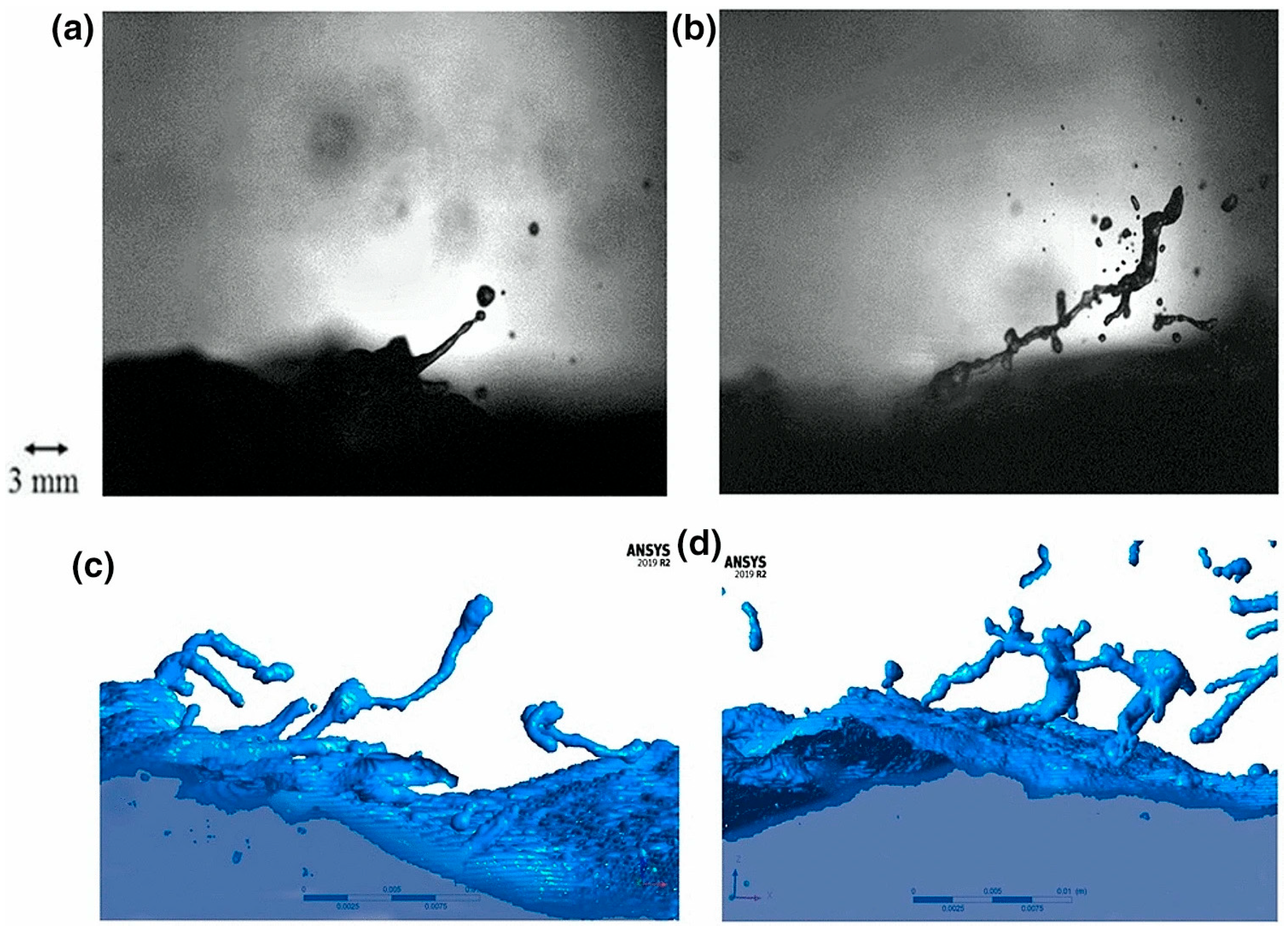
At wind speeds above about $30 {\mathrm{ms}}^{-1}$, typical of hurricanes, the character of the sea surface begins to change. Spray begins to form [19], and at yet larger wind speeds may become the rate-limiting process for air–sea fluxes [20,21]. Observations [22] and laboratory measurements [23,24] suggest that the drag coefficient ceases to rise with wind speed and may even decline. What happens to the enthalpy flux coefficient at these extreme wind speeds remains a vexing question, and field measurements and laboratory inferences show very large scatter in the estimates. Recently, it has become possible to directly simulate the formation of spray droplets e.g., [25], as shown in Figure 2.

For a simple system consisting of a semi-infinite body of pure, unstratified water surmounted by a semi-infinite, unstratified atmosphere driven by an imposed, constant horizontal pressure gradient, just three non-dimensional parameters have been identified as controlling the system dynamics [26]. Two of these depend only on gravity and the molecular properties of the two fluids. The third is defined as

$$R_u\equiv \frac{u_{\ast }^4}{\sigma g},$$

(6)

where $u_{\ast }$ is the friction velocity, $\sigma$ is the kinematic surface tension, and $g$ is the acceleration of gravity. In this simple system, the wind dependence of the character of the system should depend only on $R_u,$ which may be interpreted as the ratio of the Charnock length to the scale of the largest stable droplets in spray. For example, $R_u$ should control the fraction of the sea surface covered by whitecaps in equilibrium. In [26] it was hypothesized that all nondimensional quantities, such as the drag coefficient, should become constant in the limit of infinite $R_u$. This hypothesis has not been tested experimentally. A comprehensive review of spray-mediated turbulent fluxes may be found in [27].

What is clear at present is that boundary layer turbulence near the radius of maximum winds is a mare incognitum of tropical cyclone physics. We know from theory and numerical simulations that radial turbulent diffusion is important but we lack a quantitative theoretical model for it. Moreover, the all-important surface enthalpy and momentum fluxes are likely to be strongly affected and are perhaps rate-limited by sea spray. Research on these issues remains a critical and challenging issue in tropical cyclone physics.

3. The Outflow Layer

Observations, modeling, and theory all show that outside the hurricane’s eye the free tropical troposphere is nearly in a state of “slantwise convective adjustment” in which the temperature lapse rate is moist adiabatic along the vortex lines of the balanced flow [28]. In particular, this is true in tropical cyclone eyewalls and approximately in the outer regions [29]; here, the balanced vortex lines lie on surfaces of absolute angular momentum:

$$M=rV+\mathsf{\Omega }{r}^2,$$

(7)

where $r$ is radius, $V$ is the azimuthal velocity, assumed to be in gradient wind balance above the boundary layer, and $\mathsf{\Omega }$ is the earth’s angular velocity vector projected onto the local vertical. In an inviscid axisymmetric flow, $M$ is conserved following air motion. Moreover, $M$ increases monotonically with radius; indeed, the criterion for inertial instability is that angular momentum decrease with radius. Observations and numerical simulations confirm that $M$ increases with radius, although in the outflow layer the increase can be very slow.

The condition that the temperature lapse rate follows a moist adiabat along an angular momentum surface is equivalent to holding the saturation entropy constant on each $M$ surface, where saturation entropy is defined as the entropy air would have if water were saturated at the same pressure and temperature. From Equation (1), this quantity may be written as

$$s^{\ast }=\left(c_p+c_l{q}_t\right)\ln \left(T\right)+\frac{L_v{q}^{\ast }}{T}-\left(1+q_t\right)R_d\ln \left(p\right),$$

(8)

where $q^{\ast }$ is the mass concentration of water vapor at saturation. Convective neutrality demands that $s^{\ast }=s^{\ast }(M);$ saturation entropy is only a function of angular momentum (and time, in slowly evolving flows that maintain convective neutrality). Also, since $s^{\ast }$ is a function of pressure and temperature alone, air density can be expressed as a function of pressure and $s^{\ast }$ alone (neglecting the direct effect of water substance on air density). From this, and from gradient wind and hydrostatic balance, one can form a thermal wind relation in angular momentum coordinates [2,11,30]:

$$\frac{V}{r}=\frac{V_t}{r_t}-\left(T-T_t\right)\frac{d{s}^{\ast }}{dM},$$

(9)

where the subscript $t$ denotes evaluation at a specific point along the angular momentum surface. As one travels up an $M$ surface from the top of the turbulent boundary layer, the azimuthal velocity $V$ vanishes at some particular altitude, or temperature, which serves here as a proxy for altitude. It is convenient to define the point $t$ as that point, with radius $r_t$ and temperature $T_t$. If, furthermore, we evaluate the expression at the top of the boundary layer, Equation (9) becomes

$$\frac{V_b}{r_b}=-\left(T_b-T_t\right)\frac{d{s}^{\ast }}{dM},$$

(10)

where the subscript $b$ denotes evaluation at the top of the turbulent boundary layer. To solve Equation (10) for the azimuthal wind at the boundary layer top, we need two boundary conditions: one that determines $d{s}^{\ast }/dM$ and the other that determines $T_t$. The first is effectively a lower boundary condition and can be derived from conservation equations for entropy and angular momentum in the boundary layer. We assume that the boundary layer is well mixed in the vertical (technically, along angular momentum surfaces) and that actual entropy in the boundary layer is equal to $s^{\ast }$ just above the top of the boundary layer; this is equivalent to asserting that a sample of air in the boundary layer is neutrally buoyant when lifted moist adiabatically along angular momentum surfaces. Then the entropy and angular momentum conservation equations integrated vertically through the boundary layer are, respectively,

$$h{T}_b\frac{ds}{dt}=C_k|V_{10}|\left(k_0^{\ast }-k_{10}\right)+C_D|V_{10}{|}^3,$$

(11)

And

$$h\frac{dM}{dt}=-C_{D}r|V_{10}|V_{10},$$

(12)

where $h$ is the local depth of the boundary layer and we have approximated the temperature at the surface by $T_b$ and the radius of angular momentum surfaces in the boundary layer by $r_b$. We next take the ratio of Equations (11) to (12), which gives $ds/dM \left(=d{s}^{\ast }/dM\right)$ in the steady state, and substitute that result into (10) to give

$$V_{10}{V}_b=\frac{T_b-T_t}{T_b}\left[\frac{C_k}{C_D}\left(k_0^{\ast }-k_{10}\right)+|V_{10}{|}^2\right].$$

(13)

Comparing Equation (13) to the Carnot derivation result Equation (5), we see that the two are equivalent only if $V_{10} V_b=|V_{10}{|}^2$. The product of the gradient wind and the azimuthal wind component at the reference altitude equals the square of the magnitude of the wind (including its radial component) at the reference altitude. (Since $V_{10}<\left|V_{10}\right|,$ it follows that $V_b>\left|V_{10}\right|:$ the reference surface wind speed must be less than the gradient wind. Hurricane forecasters have long known this to be the case). Hereafter, we will make use of $V_{10} V_b=|V_{10}{|}^2$ and also make the approximation that $\left|V_{10}\right|=V_b$.

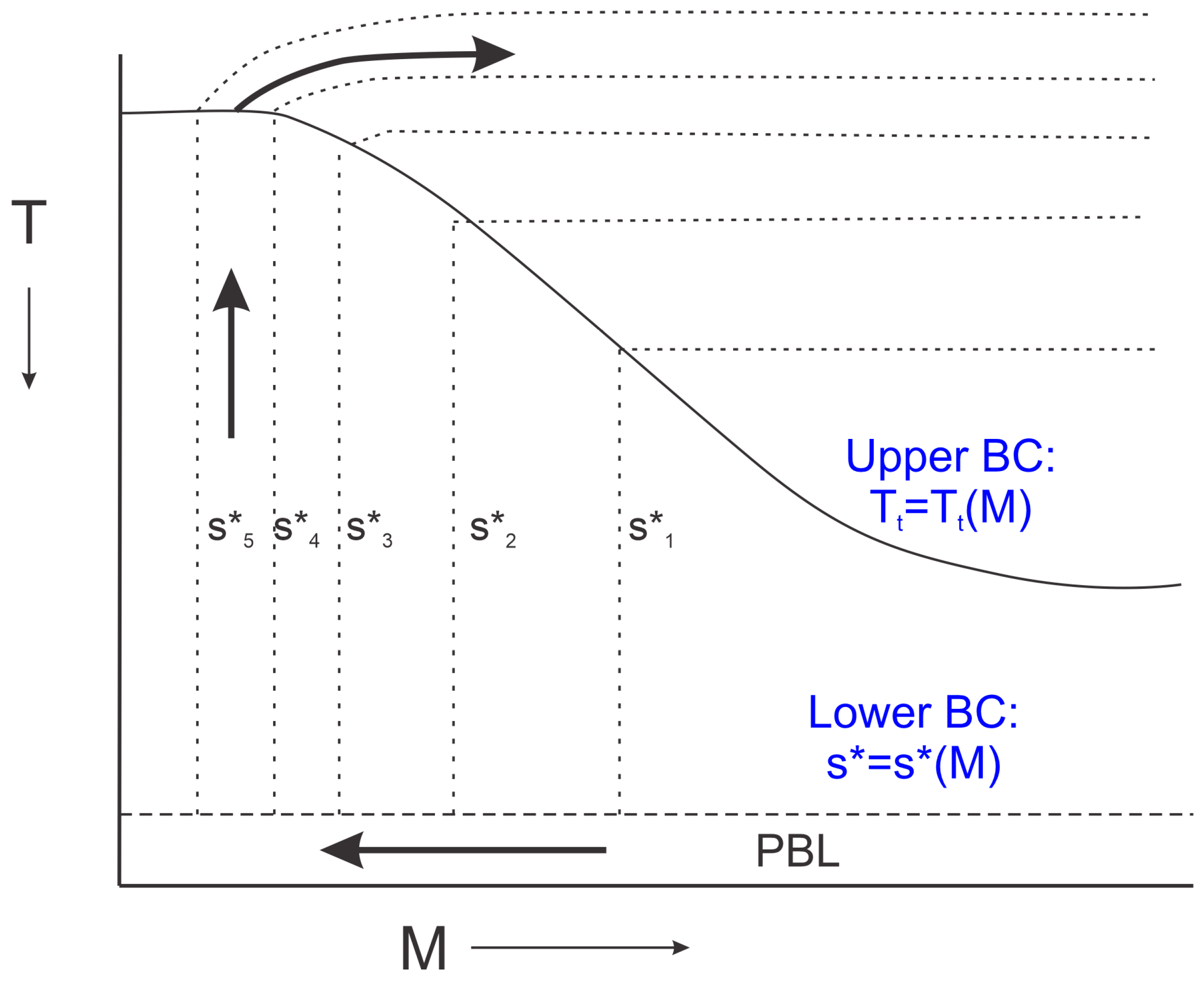
We could use Equation (13) with this approximation to predict the radial distribution of gradient wind if we knew how the temperature $T_t$ varied with angular momentum. Empirically, from detailed numerical simulations, we know that this “outflow temperature” increases as angular momentum increases [9]. In a coordinate system in which absolute temperature serves as an altitude proxy and angular momentum serves as a radial proxy, the actual situation resembles the sketch displayed in Figure 3.

The temperature at the location of vanishing azimuthal velocity increases with angular momentum. Why? The curve connecting the loci of vanishing azimuthal wind is quite certainly not the tropopause. Almost all the storm outflow lies above this curve but below or near the tropopause. In [9], we proposed that the flow near this curve was turbulent and self-stratifying, keeping the local gradient Richardson Number near its critical value for Kelvin–Helmholtz instability. We demonstrated both that the outflow is indeed quite turbulent, and the Richardson Number is near unity in a high-resolution, axisymmetric numerical simulation of a tropical cyclone. Small-scale turbulence is parameterized in this model, and production of turbulence kinetic energy shuts down when the Richardson Number exceeds unity.

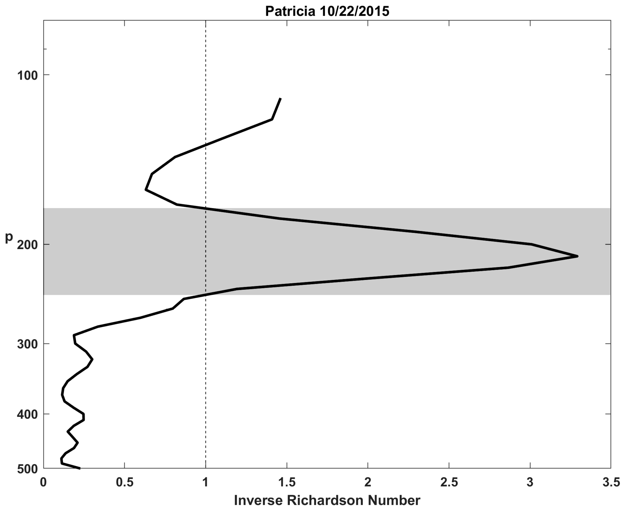
How turbulent is the outflow in real tropical cyclones? Almost all the direct measurements we have in tropical cyclones come from reconnaissance aircraft, whose maximum flight altitudes are well below the outflow of these storms. A strong desire to measure hurricane outflow was part of the motivation behind an experiment mounted by the Office of Naval Research in 2015, which deployed, among other platforms, a WB-57 aircraft capable of flying at 18 km altitude, thus overflying most tropical cyclones. The WB-57 deployed dropwindsondes, packages of in situ instruments that measure temperature, pressure, humidity, and wind speed and direction (through GPS tracking). These are parachuted down to the surface and telemeter data back to the parent aircraft.

As it happens, one of the tropical cyclones measured in the 2015 field campaign was eastern North Pacific Hurricane Patricia, which produced the highest wind speeds ever measured in a tropical cyclone. Calculations of (inverse) Richardson Number from one of the sondes that fell through Patricia’s outflow is shown in Figure 4.

The Richardson number in the outflow was quite small (large inverse Richardson Number), suggesting that the outflow was indeed turbulent.

In [16] we showed that the assumption of a critical Richardson number and taking the outflow temperature $T_t$ to be the undisturbed tropopause temperature at the storm center closes the problem and yields the complete axisymmetric structure of the steady-state tropical cyclone. For the special case of neglecting isothermal expansion effects and dissipative heating the results is

$$V_b=V_{max}\frac{r_{max}}{r}{\left[\frac{2{\left(\frac{r}{r_{max}}\right)}^2}{2-\frac{C_k}{C_D}+\frac{C_k}{C_D}{\left(\frac{r}{r_{max}}\right)}^2}\right]}^{\frac{1}{2-C_k/C_D}}-\mathsf{\Omega }r,$$

(14)

where

$$V_{max}^2={\left(\frac{1}{2}\frac{C_k}{C_D}\right)}^{\frac{\frac{C_k}{C_D}}{2-\frac{C_k}{C_D}}}\frac{C_k}{C_D}\left(T_b-T_t\right)\left({s_0}^{\ast }-{s_e}^{\ast }\right),$$

(15)

and

$$r_{max}\cong {\left(\frac{1}{2}\right)}^{\frac{1}{2}}\frac{\mathsf{\Omega }{r}_o^2}{\sqrt{\left(T_b-T_{trop}\right)\left({s_0}^{\ast }-{s_e}^{\ast }\right)}}.$$

(16)

Here ${s_0}^{\ast }$ is the saturation entropy of the sea surface (approximated as constant here) and ${s_e}^{\ast }$ is the saturation entropy of the unperturbed troposphere, another constant. The quantity $r_o$ is the “outer radius”, the distance from the storm center beyond which there is no storm-related circulation, while $r_{max}$ is the radius at which the surface winds attain their maximum value, $V_{max}.$ Note that (16) only provides a relationship between these two radii; one must specify one or the other. The theory, in its present form, does not yield an absolute radial dimension of the vortex. In nature, there is a broad range of tropical cyclone diameters that follow a log normal distribution [31,32], but we have no theory for either the median of that distribution or that predicts a log-normal distribution.

The predictions entailed by the above equations were found to describe the intensities of numerically simulated tropical cyclones quite well [9]. The predicted structure was also a good fit to numerical simulations of dry cyclones as well as those in which condensed water was not permitted to fall out of the system [6], but it failed to capture the slow decline of winds outside the storm core in moist, precipitating cyclones. In this case, the wind profile was governed by the requirement that radiative subsidence match Ekman suction at the top of the boundary layer [33].

The surprising conclusion of this analysis, to the extent that it is correct, is that turbulence in tropical cyclone outflow has a strong effect on both storm structure and intensity. It would appear that turbulence in both the boundary layer and high up in the storm circulation is essential for the existence and nature of tropical cyclones. But what, if anything, does this have to do with idealized convection between two parallel plates, about which there is an extensive literature going back to Bénard’s original 1900 paper [34]? We will explore this issue in the next section.

4. Tropical Cyclones in Parallel Plate Convection

At first glance, the preceding development bears little relationship to classical studies of parallel-plate convection. We treated a mature, steady-state vortex in isolation, with no discussion of development or as part of a systematic spatial pattern of convection. Although the theoretical development does not identify any absolute horizontal scales, natural tropical cyclones have very low aspect ratios (~1/50), whereas classical parallel-plate convection has aspect ratios of order unity. Can tropical-cyclone-like vortices develop in parallel-plate convection, and, if so, under what conditions? The first of these questions was answered as affirmative in [4], in which patterns of vortices developed in doubly periodic domains simulating rotating radiative–convective equilibrium without any phase change in water. In this case, the surface fluxes were calculated using aerodynamic flux formulae, as in the preceding development, but the compensating cooling was distributed through the interior of the fluid rather than at an upper boundary. The vortices that developed behaved much like real tropical cyclones, with low aspect ratios (but not as low as their moist counterparts).

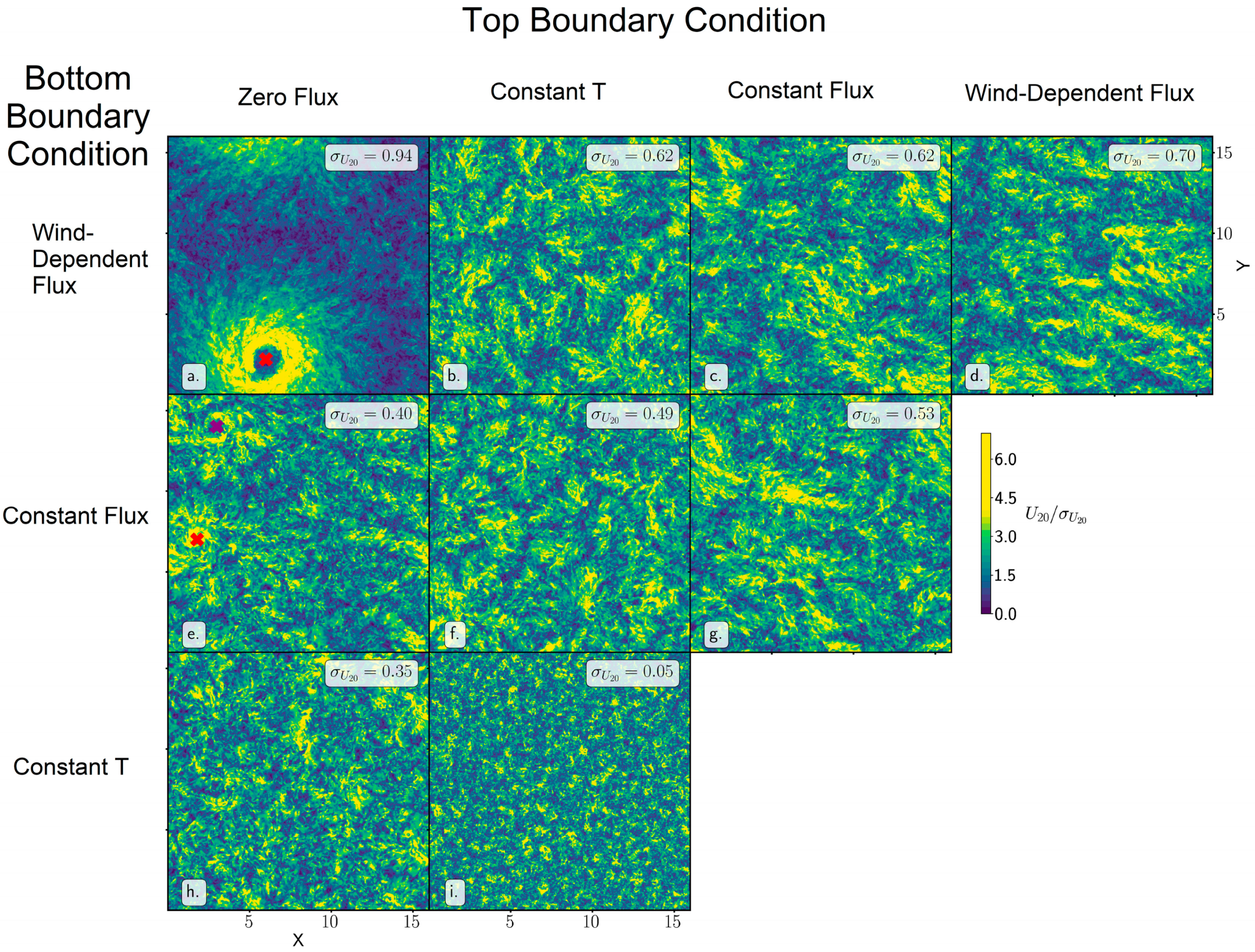
The conditions under which rotating parallel plate convection organizes into tropical cyclone-like vortices are explored in [5]. They performed direct numerical simulations of idealized, parallel-plate convection in rotating, doubly periodic domains, exploring sensitivities to both nondimensional parameters and the type of boundary condition used. In particular, they applied four types of thermal boundary conditions: constant temperature, constant flux, zero flux, and wind-dependent flux (to mimic the aerodynamic fluxes found over rough surfaces). No-slip conditions were applied on velocities, and the square domain horizontal scale was 16 times the domain depth. The governing nondimensional parameters are a flux Rayleigh number, the Prandtl Number, and a convective Rossby number, defined as

$$R{o}_c\equiv \frac{1}{2\mathsf{\Omega }}{\left(\frac{F_B}{H^2}\right)}^{\frac{1}{3}},$$

(17)

where $\mathsf{\Omega }$ is the domain angular velocity, $F_B$ is the buoyancy flux, and $H$ is the domain depth. In all the simulations, the Prandtl Number was fixed at 1.0, and for most of the simulations the flux Rayleigh Number was set to ${10}^9$, which permits moderately turbulent flows while keeping computational costs low enough to perform many simulations.

The simulations with fixed boundary temperatures produced convective patterns resembling those found in classical studies of rotating parallel-plate convection with fixed temperature at both boundaries. The aspect ratio of the convection in these cases is of order unity. With one or two constant flux or wind-dependent flux boundary conditions, larger scale structures appear, consistent with previous studies of convection with constant flux boundary conditions. But if the rotation is sufficiently slow ($R{o}_c\gtrsim 1$), tropical cyclone-like vortices appear for certain combinations of thermal boundary conditions, as shown in Figure 5.

5. Summary

Turbulence plays a critical role in tropical cyclone physics. Shear-driven turbulence near the sea surface controls the rates at which enthalpy and momentum are transferred between the ocean and atmosphere, ultimately determining the intensities of tropical cyclones that are otherwise uninfluenced by environmental interactions such as wind shear. Solutions of the equations governing steady, axisymmetric tropical cyclones also require upper boundary conditions, and, although there are no widely accepted conditions, turbulence in the outflow layer may dictate the density stratification of the outflow, which would close the solution. Such a solution has been found and is in reasonably good accord with the results of numerical simulations.

As tropical cyclones are driven by boundary heat fluxes, phase changes of water are not necessary either to simulate or to understand the phenomenon, though they do influence the intensities and structures of the resulting vortices [4]. They emerge in simulations of parallel-plate convection if the heat sink is distributed through the fluid, and the bottom thermal boundary condition is either one of constant or wind-dependent flux. We encourage those exploring parallel-plate convection to consider applying aerodynamically rough boundaries and/or distributed heat sinks/sources in the fluids.