Modal Projection for Quasi-Homogeneous Anisotropic Turbulence

Abstract

This article, or essay, addresses the anisotropic structure and the dynamics of quasi-homogeneous, incompressible turbulence. Modal projection and expansions in terms of spherical harmonics in three-dimensional Fourier space are in line with a seminal study by Jack Herring, around the so-called Craya–Herring frame of reference, with a large review of the related approaches to date. The research part is focused on structure and dynamics of rotating sheared turbulence, including a description of both directional and polarization anisotropy with a minimal number of modes. Effort is made to generalize expansions in terms of scalar spherical harmonics (SSHs) to vector spherical harmonics (VSHs). Looking at stochastic fields, for possibly intermittent vector fields, some directions are explored to reconcile modal projection, firstly used for smooth vector fields, and multifractal approaches for internal intermittency but far beyond scalar correlations, such as structure functions. In order to illustrate turbulence from Earth to planets, stars, and galaxies, applications to geophysics and astrophysics are touched upon, with generalization to coupled vector fields (for kinetic, magnetic, and potential energies), possibly dominated by waves (Coriolis, gravity, and Alfvén).

1. Introduction

The so-called ‘Craya–Herring’ frame of reference is very popular, from the seminal article of Jack Herring in 1974 [1]. Among all the scholar contributions of Herring to the physics of fluids, the modal projection is apparently a very narrow topic. Still, we show in this article that such a theme merits a large survey, with the addition of some unpublished studies. Decomposition in terms of spherical harmonics (SHs) was also touched upon by Jack Herring, so various applications of SH to scalar (SSH) and vector (VSH) fields will be discussed and compared.

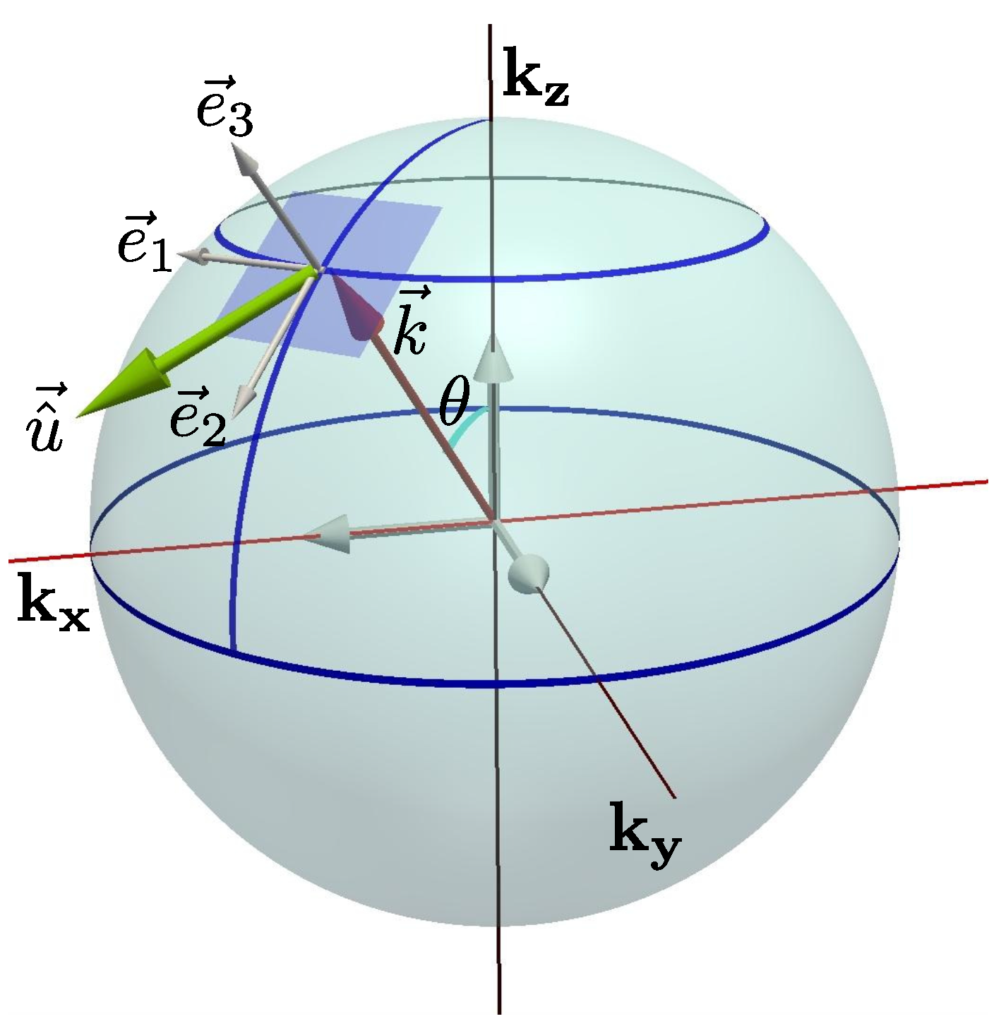
Modal projections and SH decompositions can be expressed in physical space as well as in Fourier space. It is useful to compare both of them. For instance, the so-called ‘wave–vortex’ projection by Riley et al. (1981) [2] of a solenoidal (divergence-free) fluctuating velocity field in 3D physical space has a very simple counterpart in 3D Fourier space, where it is purely algebraic and very close to the Herring’s projection. More generally, there are strong analogies between a vector field expanded on the surface of a sphere in physical space and its expansion in Fourier space. In this sense, the 3D Fourier counterpart of a solenoidal velocity field is of two components in the surface of the sphere (see Figure 1) since its radial component is zero. Such a velocity field seen in 3D Fourier space is sphéricole (from the flat animals living on the surface of a sphere, as imaged by Henri Poincaré).

Our article is organized as follows. Section 2 is devoted to a review of the related proposals for modal projection by Craya (1957) [3], Herring (1974) [1], Riley et al. (1981) [2], Cambon and Jacquin (1989) [4], and Waleffe (1992) [5], often in different contexts, with more recent analyses, mainly for linear dynamics. Applications to statistical moments, such as spectral tensors related to two-point second-order vector correlations, are addressed in Section 3. Rotating shear turbulence is investigated in Section 4 by extending the recent model by Zhu et al. (2019) [6]. In Section 5, a modal projection of poloidal/toroidal type, more general than the one related to Herring’s one, is investigated for a vector field, such as a smooth divergence-free velocity field. Promising extensions towards the stochastic modeling of possibly intermittent turbulent fields are presented from a recent project by Daniel Schertzer and followers. Section 6 is devoted to the conclusion and perspectives. Since the special issue in honor of Jack Herring is dedicated to Turbulence from Earth to Planets, Stars, and Galaxies, we end up with a list of examples of applications to geophysics and astrophysics of the technical formalism addressed in our article.

2. The Craya–Herring Frame of Reference and Beyond

Antoine Craya is known for using the eponymous frame of reference, thanks to Jack Herring (1974) [1]. Later recognized as a spectral counterpart of a general decomposition in terms of simplified toroidal/poloidal/dilatational modes, this frame leads to expressing the spectral tensors of correlation with a minimal number of scalar (or pseudo-scalar) descriptors without loss of information and for arbitrary anisotropy. Craya provided us with a special angle of attack of the so-called RDT (rapid distortion theory) and quasi-normal (QN) closures, even if he did not work directly on them. Since the original Ph.D. report from Craya (1957) is only in French and not easy to access, we recommend a recent essay with an updated survey and recent progress by the second author [7].

2.1. Related Modal Projections, Analogies, and Differences

Only a solenoidal velocity field is considered in the following. Simplified toroidal–poloidal decomposition (for a solenoidal smooth vector field u) follows from the “vortex–wave” decomposition by Riley et al. (1981) [2] with application to stably stratified turbulence:

$$\mathit{u}\left(\mathit{r}\right)=\mathbf{\nabla }\times \left(s^{\left(to\right)}\left(\mathit{r}\right)\mathit{n}\right)+\mathbf{\nabla }\times \left(\mathrm{\nabla }\times s^{\left(po\right)}\left(\mathit{r}\right)\mathit{n}\right),$$

(1)

where n is a fixed unit vector, e.g., aligned with the direction of mean stratification, and anti-parallel to the gravitational acceleration.

Leaving aside the particular application to stably stratified turbulence, this relationship is rewritten from the original reference for an easier comparison with the Craya/Herring one, from a physical space to spectral one.

The counterpart of the previous relationship in 3D Fourier space is

$$\widehat{\mathit{u}}\left(\mathit{k}\right)=𝚤{\widehat{s}}^{\left(to\right)}(\mathit{k}\times \mathit{n})-{\widehat{s}}^{\left(po\right)}\mathit{k}\times (\mathit{k}\times \mathit{n}).$$

(2)

From the relationship in physical space, it appears that the two components are individually divergence free, with a corresponding, simple orthogonality condition, in 3D Fourier space. The dependency on ${\mathit{r}}_{\Vert }=\mathit{r}·\mathit{n}$ of both $s^{\left(to\right)}$ and $s^{\left(po\right)}$, and not only on transverse variables $r_{\perp }$, is essential. If $s^{\left(to\right)}$ was independent of the axial variable $r_{\Vert }$, the toroidal component of velocity would be the same as for a two-dimensional (2D) two-component (2C) velocity field generated by a streamfunction, whereas the decomposition here is really three dimensional. A very important part of the flow, however, is zero: it was coined VSHF (vertically sheared horizontal flow) by Smith and Waleffe (2002) [8], or $\mathit{u}={\mathit{u}}_{\perp }\left(r_{\Vert }\right)$, when $\mathit{r}\Vert \mathit{n}$. Similarly, there is a hole in the representation in Fourier space for $\widehat{\mathit{u}}$, when $\mathit{k}\Vert \mathit{n}$.

A previous search towards a complete decomposition was proposed as “potosh” (poloidal/toroidal/shear) by Galmiche and Hunt [9] but it was not mathematically correct and will no longer be considered here.

The Craya–Herring decomposition was very similar to Equation (2) as

$$\widehat{\mathit{u}}\left(\mathit{k}\right)=u^{\left(1\right)}\left(\mathit{k}\right){\mathit{e}}^{\left(1\right)}\left(\mathit{\alpha }\right)+u^{\left(2\right)}\left(\mathit{k}\right){\mathit{e}}^{\left(2\right)}\left(\mathit{\alpha }\right),$$

(3)

where $({\mathit{e}}^{\left(1\right)},{\mathit{e}}^{\left(2\right)},\mathit{\alpha }=\mathit{k}/k)$ form a direct orthonormal frame of reference for a given orientation of the wave vector k as shown in Figure 1. At this stage, the case $k_{\perp }=0$ is puzzling and ought to be treated as a singular point. The unit vector ${\mathit{e}}^{\left(1\right)}$, defined as

$${\mathit{e}}^{\left(1\right)}=\frac{\mathit{k}\times \mathit{n}}{\mid \mathit{k}\times \mathit{n}\mid },$$

with $k_{\perp }=\mid \mathit{k}\times \mathit{n}\mid$, is not defined for $k_{\perp }=0$, or, more precisely, it must be defined as a limit that depends on the angle $\varphi$ in polar-spherical coordinates, following a given meridian towards the pole of the sphere. In short, the VSHF is accounted for in the Craya–Herring frame, but it corresponds to $k_{\perp }=0$ so that it is concerned by the possible polar multi-definitions of the local frame.

The orthonormal frame is recovered by Ying et al. (2019) [6] for the gradient operator in k-space, passing from Cartesian coordinates to polar-spherical ones, with

$$k\frac{\partial }{\partial k_n}={\alpha }_{n}k\frac{\partial }{\partial k}+e_n^{\left(2\right)}\frac{\partial }{\partial \theta }-\frac{e_n^{\left(1\right)}}{sin\theta }\frac{\partial }{\partial \varphi },$$

(4)

where $\theta$ is the polar angle (on Figure 1) and $\varphi$ the azimuthal angle.

Since the $\widehat{\mathit{u}}$ vector related to a solenoidal (divergence-free) vector in physical space is of two components in the plane normal to the wave vector, it is interesting to use complex-valued base vectors to project $\widehat{\mathit{u}}$, or

$$\mathit{N}\left(s\mathit{\alpha }\right)={\mathit{e}}^{\left(2\right)}\left(\mathit{\alpha }\right)-s𝚤{\mathit{e}}^{\left(1\right)}\left(\mathit{\alpha }\right),s=\pm 1.$$

(5)

Introduced by Cambon and Jacquin (1989) [4] in order to study nonlinear rotating turbulence, they were coined helical modes by Waleffe (1992). They are eigenmodes of the Curl operator, as $\mathit{N}(\pm k)\mathbf{exp}(\pm \mathit{𝚤}\mathit{k}·\mathit{x})$. They simplify the basic equations, even without basic rotation, from the expression of the Lamb vector in 3D Fourier space $\widehat{\mathit{\omega }\times \mathit{u}}$, and allow to ensure the solenoidal constraint $(\mathbf{\nabla }·\mathit{u}=0$, $\mathit{k}·\widehat{\mathit{u}}=0)$, in avoiding the byzantine use of projectors (as jokingly said by Leaf Turner, Los Alamos). In addition, they diagonalize the operator of inertial waves in a rotating frame. The helical decomposition can be written as

$$\widehat{\mathit{u}}\left(\mathit{k}\right)=\sum _{s=\pm 1}{u}_s\left(\mathit{k}\right)\mathit{N}\left(s\mathit{\alpha }\right),$$

(6)

for the velocity fluctuation.

2.2. Including Other Coupled Fields, Buoyancy, Magnetic Field

It is possible to include the buoyancy scalar b in stratified turbulence in a new 3D-3C vector as

$$\mathit{w}\left(\mathit{k}\right)=\widehat{\mathit{u}}\left(\mathit{k}\right)+𝚤\frac{\widehat{b}}{N}\mathit{\alpha },$$

(7)

where N is the Brunt–Wäisälä frequency so that $b/N$ has the dimension of a velocity. The Hermitian symmetry holds with the factor 𝚤, and $(1/2){\widehat{b}}^{\ast }·\widehat{b}/N^2$ is related to the density of potential energy as $(1/2){\widehat{\mathit{u}}}^{\ast }·\widehat{\mathit{u}}$ for the kinetic energy.

As for MHD flows, a few independent variables can generate both the velocity and the magnetic fields, both being divergence-free vectors.

3. Application to Two-Point Second Order Statistics for Strong Anisotropy

In arbitrary incompressible HAT (homogeneous anisotropic turbulence), the spectral tensor ${\widehat{R}}_{ij}\left(\mathit{k}\right)$ is the 3D Fourier transform of the two-point second-order correlation tensor

$$R_{ij}\left(\mathit{r}\right)=\langle u_i\left(\mathit{x}\right)u_j(\mathit{x}+\mathit{r})\rangle .$$

(8)

Its general form calls into play three contributions [4]:

$${\widehat{R}}_{ij}\left(\mathit{k}\right)=\mathcal{E}\left(\mathit{k}\right)P_{ij}\left(\mathit{\alpha }\right)+\Re \left(Z\left(\mathit{k}\right)N_i{N}_j\right)+𝚤{ϵ}_{ijn}{\alpha }_n\mathcal{H}\left(\mathit{k}\right),P_{ij}\left(\mathit{\alpha }\right)={\delta }_{ij}-{\alpha }_i{\alpha }_j.$$

(9)

The relationship (9) involves two scalars (energy and helicity spectra) and one complex-valued pseudo-scalar Z for polarization anisotropy. The energy spectrum is related to the trace, or $\mathcal{E}=(1/2){\widehat{R}}_{ii}$, and the helicity spectrum $k\mathcal{H}\left(\mathit{k}\right)$ is related to the purely imaginary and antisymmetric part of ${\widehat{R}}_{ij}$. Last but not least, the real and symmetric deviatoric contribution from polarization, $R_{ij}^{\left(\mathrm{pol}\right)}=\Re \left(Z{N}_i{N}_j\right)$ is much less known: It is generated by Z, using the helical modes or directly extracted from the spectral tensor in Cartesian coordinates, from

$${\widehat{R}}_{ij}^{\left(\mathrm{pol}\right)}\left(\mathit{k}\right)=\frac{1}{2}\left(P_{im}{P}_{jn}+P_{in}{P}_{jm}-P_{ij}{P}_{mn}\right){\widehat{R}}_{mn}\left(\mathit{k}\right).$$

(10)

Of course, the latter equation, which also corresponds to $Z\left(\mathit{k}\right)=(1/2){\widehat{R}}_{mn}{N}_m^{\ast }{N}_n^{\ast }$, is tautological. Our goal is to replace ${\widehat{R}}_{mm}$ in the latter equations with a simpler tensor, to which classical or modified SH expansions may apply.

The first term of Equation (9) can be split into a purely 3D isotropic part and a part that reflects directional anisotropy, or

$$\mathcal{E}\left(\mathit{k}\right)P_{ij}\left(\mathit{\alpha }\right)=\frac{E\left(k\right)}{4\pi k^2}{P}_{ij}\left(\mathit{\alpha }\right)+{\widehat{R}}_{ij}^{\left(\mathrm{dir}\right)}\left(\mathit{k}\right),$$

with

$${\widehat{R}}_{ij}^{\left(\mathrm{dir}\right)}\left(\mathit{k}\right)=\left(\mathcal{E}\left(\mathit{k}\right)-\frac{E\left(k\right)}{4\pi k^2}\right)P_{ij}\left(\mathit{\alpha }\right).$$

(11)

In the presence of the advected scalar field b, an extended spectral tensor can be defined from Equation (7) as

$$\langle w_i^{\ast }\left(\mathit{p}\right)w_j\left(\mathit{k}\right)\rangle =W_{ij}\left(\mathit{k}\right){\delta }^3(\mathit{k}-\mathit{p}).$$

(12)

From the augmented $\mathbf{W}$ tensor vs. $\widehat{\mathbf{R}}$, additional spectra for potential energy and for toroidal and poloidal buoyancy fluxes are readily defined.

Similarly for MHD flows, the $(\mathcal{E},Z,\mathcal{H})$ set for the kinetic flow is complemented by a magnetic set $({\mathcal{E}}^M,Z^M,{\mathcal{H}}^{\mathcal{M}})$ with the same structure, whereas magnetic–kinetic co-spectra involve the cross helicity, the vector field of the electromotive force, and two unnamed cross-polarization terms. (see [10], Chapter 12).

3.1. Decomposition in Terms of Scalar Spherical Harmonics (SSH)

Regarding the smooth statistical terms $\mathcal{E}$, $\mathcal{H}$, they are true scalar terms, invariant to any change of the orthonormal frame so that they can be expanded in terms of SSH. The same property is valid for the modulus $\mid Z \mid$ of the polarization term but not for Z as a whole. For instance, a SO(3)-type expansion holds for the scalar $\mathcal{E}$ as

$$\mathcal{E}\left(\mathit{k}\right)=\frac{E\left(k\right)}{4\pi k^2}\left(1+H_{mn}^{2\left(\mathrm{dir}\right)}\left(k\right){\alpha }_m{\alpha }_n+H_{mnpq}^{4\left(\mathrm{dir}\right)}\left(k\right){\alpha }_m{\alpha }_n{\alpha }_p{\alpha }_q+\cdots \right).$$

(13)

This expansion was established in several papers, quoted in [10]. A very useful identity is

$$H_{ij}^{2\left(\mathrm{dir}\right)}=-15H_{ij}^{\left(\mathrm{dir}\right)},$$

(14)

where $2E\left(k\right)H_{ij}^{\left(\mathrm{dir}\right)}\left(k\right)$ is the spherical integral (integral on the surface of a sphere of radius $k=\mid \mathit{k}\mid$) of ${\widehat{R}}_{ij}^{\left(\mathrm{dir}\right)}$ in Equation (11). Nevertheless, it is difficult to extend a practical expansion beyond degree 2 (degree 4 by Rubinstein et al. (2015) [11] and Briard (2017) [12]).

Accordingly, the classical expansion in terms of scalar spherical harmonics is much more practical, especially when the degree increases:

$$\mathcal{E}\left(\mathit{k}\right)=\frac{E\left(k\right)}{4\pi k^2}\left(1+\sum _{n=1}^N\sum _{m=-2n}^{2n}{e}_{2n}^m\left(k\right)Y_{2n}^m(\theta ,\varphi )\right),$$

(15)

in which $Y_n^m(\theta ,\varphi )$ are expressed in terms of extended Legendre polynomials $P_n^m\left(\theta \right)$ via

$$Y_n^m(\theta ,\varphi )=P_n^m\left(\theta \right)exp\left(𝚤m\varphi \right).$$

(16)

$2n$ is called the degree, only even here, up to a maximum $2N$, and m is the order that is limited by $2n$. In contrast with the expansion in terms of tensors, the properties of orthogonality are obvious. The basis depends on the choice of the polar axis but not the degree so that at any given degree, there are simple linear relationships to pass from $Y_n^m(\theta ,\varphi )$ to $Y_n^{\prime m}({\theta }^{\prime },{\varphi }^{\prime })$ from a system of polar-spherical coordinates to another one.

Only even degrees are relevant, from the Hermitian symmetry restricted to a purely real term. Note that the number of degrees of freedom is recovered from the tensorial decomposition to the scalar spherical one: at degree 2, there are five $e_2^m\left(k\right)$ descriptors, with $m=-2,-1,0,1,2$, and five independent components for the symmetric traceless tensor $H_{ij}^{\left(\mathrm{dir}\right)}\left(k\right)$.

3.2. Angular Harmonics for the Polarization Term

The decomposition in terms of spherical harmonics was touched upon by Jack Herring for homogeneous axisymmetric turbulence with mirror symmetry. In this case, the two-point second order spectral tensor reduces to two components only:

$${\Phi }^{11}(k,\theta )={\widehat{R}}_{ij}{e}_i^{\left(1\right)}{e}_j^{\left(1\right)}and{\Phi }^{22}(k,\theta )={\widehat{R}}_{ij}{e}_i^{\left(2\right)}{e}_j^{\left(2\right)}.$$

(17)

For this particular symmetry, it was proposed to expand both ${\Phi }^{11}$ and ${\Phi }^{22}$ in terms of the simple Legendre polynomials $P_n^0\left(\theta \right)$. This was correct for the spectral energy, or $(1/2)({\Phi }^{11}+{\Phi }^{22})$, but not for the polarization counterpart, or $(1/2)({\Phi }^{22}-{\Phi }^{11})$, which reduces to Z. In effect, Z may vanish at the pole in the axisymmetric case. This suggests restricting the expansion in terms of the simple Legendre polynomials to $\mathcal{E}$ and to $\tilde{Z}$ with $Z={sin}^2\theta \tilde{Z}$.

From the simple example of axisymmetric turbulence, it is clear that the SSH expansion cannot be applied directly to Z. Setting aside a possible direct application of VSH, in Section 5, a simpler method is first proposed. Its goal is to solve, beyond the axisymmetric case, the problem of the special definition or multiple definition of a vector field in the Craya–Herring frame of reference that implies a similar problem for Z.

For this purpose, one recovers the decomposition by CC and Teissèdre (1985) [13] as

$$Z\left(\mathit{k}\right)={sin}^2{\theta }_k\tilde{Z}\left(\mathit{k}\right)-{\left(\frac{1+cos{\theta }_k}{2}\right)}^{2}exp\left(2𝚤{\varphi }_k\right)\Psi \left(k\right)-{\left(\frac{1-cos{\theta }_k}{2}\right)}^{2}exp(-2𝚤{\varphi }_k){\Psi }^{\ast }\left(k\right),$$

(18)

in which $\Psi$ derives from the value of ${\widehat{R}}_{ij}(k,\mathit{n})$ exactly at the pole $\mathit{\alpha }=\mathit{n}$:

$$\Psi =\frac{1}{2}\left({\widehat{R}}_{22}-{\widehat{R}}_{11}+𝚤\left({\widehat{R}}_{12}+{\widehat{R}}_{21}\right)\right).$$

(19)

This equation derives from the calculation of $(1/2)N_i^{\ast }{N}_j^{\ast }{\Psi }_{ij}\left(\mathit{k}\right)$: The choice ${\Psi }_{ij}\left(\mathit{k}\right)={\widehat{R}}_{ij}(k,\mathit{n})+{sin}^2{\theta }_k{\tilde{\Psi }}_{ij}\left(\mathit{k}\right)$ yields Equation (18). This equation expresses explicitly the multidefinition of Z at the exact pole, with $Z\to -exp\left(2𝚤{\varphi }_k\right)\Psi$. Accordingly, $\Psi$ in Equations (18) and (19) is the continuous limit of Z at ${\varphi }_k=\pi /2$, but this is not the case in following any other meridian line (fixed ${\varphi }_k$) when converging towards the pole. In the whole spectral domain, this equation can be considered as exact provided that ${\widehat{R}}_{ij}\left(\mathit{k}\right)-{\widehat{R}}_{ij}(k,\mathit{n})$ behaves as ${sin}^2{\theta }_k$. The particular axisymmetric case corresponds to $\Psi =0$, $\tilde{Z}=\tilde{Z}(k,{\theta }_k)$.

Z cannot be expanded in terms of $Y_n^m$, but Equation (18) suggests transferring the decomposition in terms of scalar spherical harmonics from Z to $\tilde{Z}$, and the preliminary results of CC and Teissèdre (1985) were encouraging [13]. In this case, $\Psi$ gives the polarization of the spectral tensor exactly at the pole, and a correct convergence to this polar value is ensured, with

$$\tilde{Z}=\sum _{n=0}^N\sum _{m{=}_n}^n{z}_n^m\left(k\right)Y_n^m(\theta ,\varphi ),$$

with both even and odd degrees. Coefficients with odd degrees are imaginary.

As another good property, Equation (18) and the latter is consistent with the degree 2, or

$$Z(\mathit{k},t)=\frac{5}{2}{N}_i^{\ast }\left(\mathit{\alpha }\right)N_j^{\ast }\left(\mathit{\alpha }\right)H_{ij}^{\left(\mathrm{pol}\right)}(k,t),$$

with $\Psi \left(k\right)=\frac{5}{2}(H_{22}^{\left(\mathrm{pol}\right)}-H_{11}^{(\mathrm{pol}}+2𝚤H_{12}^{\left(\mathrm{pol}\right)})$ and $\tilde{Z}\left(k\right)=\frac{5}{2}(2H_{33}^{\left(\mathrm{pol}\right)}-H_{11}^{\left(\mathrm{pol}\right)}-H_{22}^{(\mathrm{pol}})$.

Because Z represents the tensor of polarization, it is interesting to go beyond SSH, and to look at vectorial spherical harmonics (VSH); if a decomposition is valid for a vector V, it should apply to a tensor, forming $\mathit{V}\otimes \mathit{V}$.

Even if physical data for the anisotropic helicity spectrum are missing in HAT, an SSH decomposition can be proposed, similarly to (13) and (15) but with additional, purely imaginary, terms of odd degrees.

Going back to the SO(3)-type expansion, a general one can be proposed as

$$Z\left(\mathit{k}\right)=\frac{1}{2}\frac{E\left(k\right)}{4\pi k^2}\left(H_{ij}^{2\left(\mathrm{pol}\right)}\left(k\right)+𝚤H_{ijm}^{3\left(\mathrm{pol}\right)}\left(k\right){\alpha }_m+H_{ijmn}^{4\left(\mathrm{pol}\right)}{\alpha }_m{\alpha }_n+\cdots \right)N_i^{\ast }\left(\mathit{\alpha }\right)N_j^{\ast }\left(\mathit{\alpha }\right).$$

(20)

Note that the terms with odd degrees yield imaginary contributions from generating k-modulus tensors. As for the energy spectrum, the identity

$$H_{ij}^{2\left(\mathrm{pol}\right)}\left(k\right)=5H_{ij}^{\left(\mathrm{pol}\right)}\left(k\right),$$

(21)

holds, in which $2E\left(k\right)H_{ij}^{\left(\mathrm{pol}\right)}\left(k\right)$ is the spherical integral of ${\widehat{R}}_{ij}^{\left(\mathrm{pol}\right)}\left(k\right)$. In addition, terms of degree 3 and 4 were investigated by Briard (2017) [12] but without a practical and systematic way to reach higher degrees (see also Rubinstein et al. (2015) [11]).

4. SSH Decomposition in Rotating Shear Turbulence

In this section, let us concentrate on rotating shear flows. We begin by reviewing the ZCG model and the numerical simulations based on it, with typical combinations of mean shear and system rotation. Using the simulation data, we evaluate the equivalency of the tensorial expansion of the SO(3) type and the SSH decomposition on the $\mathcal{E}$ field. Then, by expanding $\mathcal{E}$ and $\left|Z\right|$ to high degrees using SSH, we explore the anisotropy-generating mechanism by the linear operator and anisotropy damping induced by nonlinear terms of ZCG.

4.1. Recalling ZCG Model

ZCG is a statistical spectral model developed for homogeneous anisotropic turbulence by the author Y. Zhu, C. Cambon, and our collaborator F. S. Godeferd. For all relevant formulas, numerical details, and simulation results presented in this section, part of them are published in Zhu et al. (2019) [6], and the other unpublished part is in the Ph.D. thesis of the first author [14].

4.1.1. Spectral Models for Homogeneous Anisotropic Turbulence

Consider an extensional mean flow with a spatially uniform mean-velocity gradient $A_{ij}=S_{ij}+\frac{1}{2}{ϵ}_{imj}{\mathcal{W}}_m$, under a solid body rotation of the frame with the angular velocity $\mathbf{\Omega }$, The governing equation for $(\mathcal{E},Z)$ ($\mathcal{H}$ is neglected) reads

$$\begin{array}{cc}\hfill & \dot{\left(k\mathcal{E}\right)}+2\nu k^3\mathcal{E}+\Re \left(kZ(k,t)S_{ij}{N}_i\left(\mathit{\alpha }\right)N_j\left(\mathit{\alpha }\right)\right)=k{T}^{\left(\mathcal{E}\right)}(\mathit{k},t),\hfill \end{array}$$

(22a)

$$\begin{array}{cc}\hfill & \dot{\left(kZ\right)}+2\nu k^{3}Z+k\mathcal{E}(\mathit{k},t)S_{ij}{N}_i(-\mathit{\alpha })N_j(-\mathit{\alpha })-𝚤kZ(k,t)\left((\mathcal{W}+4\mathbf{\Omega })·\mathit{\alpha }-2{\Omega }_E\right)=k{T}^{\left(Z\right)}(\mathit{k},t).\hfill \end{array}$$

(22b)

The overdot denotes the advection operator due to the presence of the mean flow, namely $\dot{(...)}=\frac{\partial }{\partial t}-A_{mn}{k}_m\frac{\partial }{\partial k_n}$. $\nu$ is the kinetic viscosity. ${\Omega }_E$ is the rotation rate induced by the advection operator, which can be removed by applying special A and n. Equation (22) derives from the Navier–Stokes equations (NSE). The left-hand side (LHS) of Equation (22) represents the linear effects of the mean flow as in viscous linear spectral theory (SLT), which was originally developed as RDT (see [15,16]). Note that the LHS of (22a) and (22b) contains viscous terms and similar terms from strain S (the symmetric part of the mean-velocity gradients), but the antisymmetric part of the mean-velocity gradients (the mean vorticity $\mathcal{W}$) only affects the equation for polarization through a combination with the system vorticity $4\mathbf{\Omega }$ (the ‘stropholysis’ effect coined by [17]). The right-hand side (RHS) of Equation (22) gathers the contribution from two-point third-order correlations mediated by the quadratic nonlinearity of basic NSE that should be closed properly depending on the flow regime and available computational resources.

Previous studies developed a series of sophisticated and successful models based on the high-order closures using the eddy damped quasi-normal Markovian (EDQNM) technique. The EDQNM closure was first built by Orszag for homogeneous isotropic turbulence (HIT) (see [18]), later extended to shear-driven flow and flows driven by buoyancy or coupled fields, such as magneto-hydrodynamics (see review in [10,19]). Concerning shear-driven flows, various formulations and resolution methods can be chosen. For example, EDQNM-1—the model derived for turbulent flows when linear terms are associated with energy production in double correlation equations—keeps the full angular dependence in (22). The model of EDQNM-1 type for unstably stratified homogeneous turbulence in [20] compares well with direct numerical simulation (DNS), but EDQNM-1 for a purely anisotropic velocity field has not been implemented because of the complicated and computationally expensive 3D convolutions involved with the $T^{\left(\mathcal{E}\right)}$ and $T^{\left(Z\right)}$ terms. A simplified model from EDQNM-1—MCS (see [21])—gives the spherically averaged descriptors that depend on radius k by retaining only the first two degrees of the angular harmonics of $\mathcal{E}\left(k\right)$ and $Z\left(k\right)$ in (13) and (20). Although validated for different flows, the MCS model shows that it is much less adapted to the representation of angular variations for linear terms than for nonlinear terms based on long-term comparisons with SLT and DNS.

The ZCG model was designed to restore the full angular dependence of linear terms in the equations for $\mathcal{E}(\mathit{k},t)$ and $Z(\mathit{k},t)$, as in EDQNM-1, and to restrict to nonlinear transfer terms $T^{\left(\mathcal{E}\right)}$ and $T^{\left(Z\right)}$ the use of low-degree expansion inspired by MCS. Additionally, to include the effect from the anisotropy higher than degree 2, ZCG added return-to-isotropy (RTI) terms to $T^{\left(\mathcal{E}\right)}$ and $T^{\left(Z\right)}$ as

$$\begin{array}{cc}\hfill T^{\left(\mathcal{E}\right)}(\mathit{k},t)=& T^{\left(\mathcal{E}\right)2}(\mathit{k},t)-{\phi }^{\left(\mathrm{RTI}\right)}(k,t)\left(\mathcal{E}(\mathit{k},t)-{\mathcal{E}}^{\left(2\right)}(\mathit{k},t)\right)\hfill \\ \hfill T^{\left(Z\right)}(\mathit{k},t)=& T^{\left(Z\right)2}(\mathit{k},t)-{\phi }^{\left(\mathrm{RTI}\right)}(k,t)\left(Z(\mathit{k},t)-Z^{\left(2\right)}(\mathit{k},t)\right).\hfill \end{array}$$

(23)

$T^{\left(\mathcal{E}\right)2}(\mathit{k},t)$ and $T^{\left(Z\right)2}(\mathit{k},t)$ are reconstructed from spherically averaged nonlinear descriptors ${\tilde{S}}_{ij}^{\mathrm{NL}\left(\mathrm{dir}\right)}(k,t)$ and ${\tilde{S}}_{ij}^{\mathrm{NL}\left(\mathrm{pol}\right)}(k,t)$ given by MCS, as an analogy to (13) and (20), truncated at degree 2. ${\mathcal{E}}^{\left(2\right)}(\mathit{k},t)$ and $Z^{\left(2\right)}(\mathit{k},t)$ are the exact first two-degree components of (13) and (20), respectively. ${\phi }^{\left(\mathrm{RTI}\right)}(k,t)$ is borrowed from Weinstock’s model [22,23], in which only isotropic EDQNM is employed for the nonlinear closure, other than MCS.

Solving the advection operators in (22) is the main challenge for numerically simulating ZCG. In the commonly used approach of SLT, as well as in fully nonlinear DNS by Rogallo (1981) [24] and Lesur and Longaretti (2005) [25], the scheme amounts to following the characteristic lines in terms of $\mathit{k}\left(t\right)$ related to the mean Lagrangian trajectories in physical space. As a result, the wave vector is time dependent so that the time evolution of a statistical quantity $\Phi$ appears as $\dot{\Phi }(\mathit{k}\left(t\right),t)={\displaystyle \frac{\partial \Phi }{\partial t}}+{\displaystyle \frac{\partial \Phi }{\partial k_i}}{\displaystyle \frac{\mathrm{d}{k}_i}{\mathrm{d}t}}$ with ${\dot{k}}_i=-A_{ji}{k}_j$ the eikonal equation. To avoid the distorted grids in the conventional method, which are difficult to couple with nonlinear models based on spherically averaged descriptors, the ZCG model uses a finite-difference scheme for evaluating the $\partial /\partial k_i$ derivatives (4), with a discretization of the wave vector consistent with the polar-spherical coordinates presented in Figure 1. To fix the multi-definition of $Z(\mathit{k},t)$ at the pole, we look backward to the $\widehat{\mathbf{R}}(\mathit{k}.t)$ equation in a small region around the pole. Readers can find the special treatment of the pole zone in Appendix A.

4.1.2. Numerical Simulations for Rotating Shear Flows

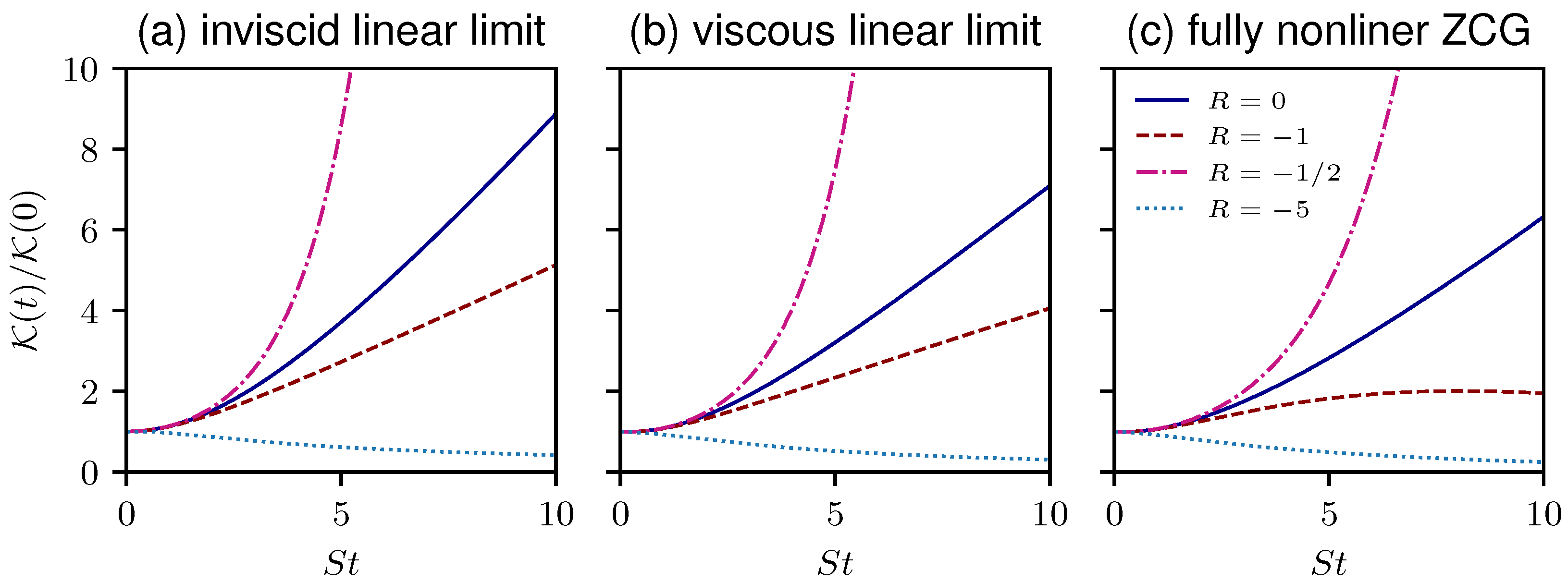
Among various combinations of mean-flow gradients and system rotation, the rotating shear flow with the mean plane shear rotating in the spanwise direction is of great interest for its widespread applications from engineering—e.g., turbomachinery or hydroelectric power generation—to geophysics and astrophysics. Previous studies with SLT (spectral linear theory), e.g., ref. [16] for rotating shear turbulence, ref. [26] for stratified shear flows and [27] for rotating stratified shear turbulence, show the global relevance of the Bradshaw number B (see [28]) for characterizing the stability of rotating shear flow: $B=R(R+1)$, in which the Rossby number $R=2\Omega /-S$ is the ratio of system vorticity $\Omega$ to shear-induced vorticity $-S$. Cases with $B<0$ or $-1<R<0$ correspond to the exponential growth of turbulent kinetic energy, and $B>0$ to exponential decay. Neutral cases are found for $R=0$ (no background rotation) and $R=-1$ (zero absolute vorticity). Accordingly, four typical rotating shear flows (with various values of R) are numerically simulated in [6] by ZCG, namely using (22) and (23): $R=-5$ corresponds to a stabilizing, anticyclonic case; $R=-1$ for a neutral case with zero absolute vorticity, as encountered in the central region of a rotating channel; $R=-1/2$ for a maximum destabilization, anticyclonic case, as in the pressure side of a rotating channel; and $R=0$ with no rotation. The mean shear and system rotation are chosen as $A_{ij}=S{\delta }_{i1}{\delta }_{j2}$ and $\mathbf{\Omega }=\Omega {\delta }_{i3}$, respectively, to vanish the term of ${\Omega }_E$ in Equation (22).

We first carried out the simulations in the linear limit (namely setting the RHS of Equation (22) zero), with $\nu =0$ (the inviscid linear limit) and $\nu \ne 0$ (the viscous linear limit), respectively. The ZCG model showed an almost perfect coincidence of the results, compared to their corresponding ones obtained by the STL for all four values of R and compared to the analytical results for the pure shear case when $R=0$. Then, we turned on the RHS of Equation (22), i.e., simulating the fully nonlinear ZCG model, and compared the data to those obtained by Sahli et al. [29] using DNS. Great agreement of the results between ZCG and DNS for all the four typical values of R firmly validated our ZCG model. It is interesting that although MCS failed in most cases, it succeeded in generating exponentially increasing energy in the maximum destabilization case ($R=-1/2$). Figure 2 presents the time evolution of the kinetic energy $\mathcal{K}\left(t\right)={\int }_0^{\infty }E(k,t)\mathrm{d}k$ by simulating ZCG, with various Rossby numbers, in the three different limits.

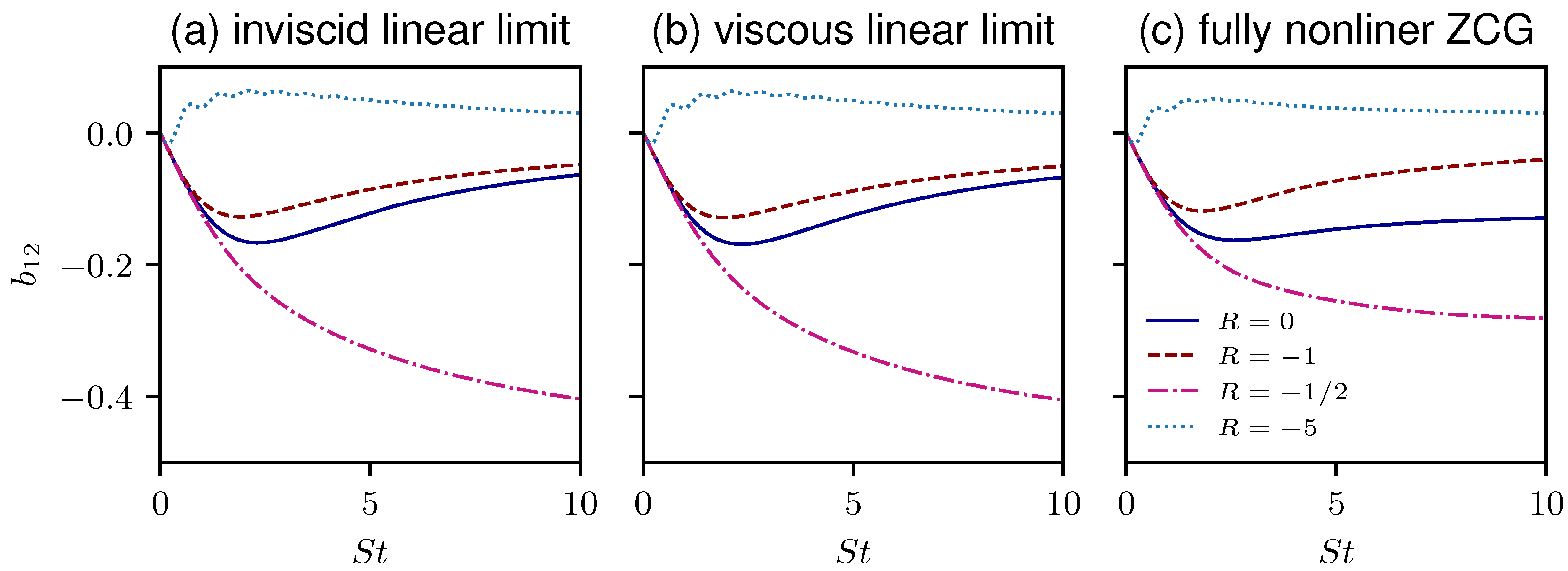
Figure 3 exhibits the according time evolution of the deviatoric part of the Reynolds stress tensor $b_{12}$, which is the Reynolds stress tensor component $R_{12}=\langle u_1\left(\mathit{x}\right)u_2\left(\mathit{x}\right)\rangle$ non-dimensionalized by $2\mathcal{K}$, and plays an important role in the energy injection by the mean shear. The most remarkable achievement in [6] is that the fully nonlinear ZCG accomplished the clearly steady limit of $b_{12}=-0.14$ in the pure shear case (see Figure 3c), with a constant value very close to the classically expected one, in the range [−0.16; −0.1] (see table p. 443 in [10]), and thereby provided the exponential re-growth of energy (see Figure 2c), for the first time as a spectral model.

4.2. Numerical Validation of the Equivalency of SO(3) Expansion and SSH Decomposition

Here, we use the simulation data introduced above by the ZCG model to validate the equivalency of the tensorial expansion (of SO(3) type) and the SSH decomposition of a scalar field, with their applications on $\mathcal{E}\left(\mathit{k}\right)$ firstly.

Rubinstein et al. [11] pointed out some properties of the coefficient tensors in the SO(3)-type expansion (13): They can be assumed symmetric under any interchange of indices and also trace free in the extended sense that the contraction of any two indices vanishes identically. There are $2n+1$ linearly independent tensors with this property for each degree $2n$. Note that degree zero corresponds to the isotropic part ${\displaystyle \frac{E\left(k\right)}{4\pi k^2}}$, and the second degree is found as $H_{ij}^{2\left(\mathrm{dir}\right)}=-15H_{ij}^{\mathrm{dir}}$, which is applied on MCS. Rubinstein et al. [11] extended a practical expansion for degree 4, as

$$E\left(k\right)H_{mnpq}^{4\left(\mathrm{dir}\right)}=\underset{S_k}{\int \int }\mathcal{E}\left(\mathit{k}\right)P_{mnpq}\left(\mathit{\alpha }\right){\mathrm{d}}^2\mathit{k},$$

(24)

with

$$\begin{array}{cc}\hfill P_{ijpq}\left(\mathit{\alpha }\right)=& {\alpha }_i{\alpha }_j{\alpha }_p{\alpha }_q-\frac{1}{7}({\delta }_{ij}{\alpha }_p{\alpha }_q+{\delta }_{ip}{\alpha }_j{\alpha }_q+{\delta }_{iq}{\alpha }_j{\alpha }_p\hfill \\ \hfill & +{\delta }_{jp}{\alpha }_i{\alpha }_q+{\delta }_{jq}{\alpha }_i{\alpha }_p+{\delta }_{pq}{\alpha }_i{\alpha }_j)+\frac{1}{35}\left({\delta }_{ij}{\delta }_{pq}+{\delta }_{ip}{\delta }_{jq}+{\delta }_{iq}{\delta }_{pj}\right).\hfill \end{array}$$

(25)

It is unrealistic to extend to higher expression for its complexity.

To compare the results, we denote

$${\mathcal{E}}^0\left(\mathit{k}\right)=\&{\mathcal{E}}^{0\left(\mathrm{T}\right)}\left(\mathit{k}\right)={\mathcal{E}}^{0\left(\mathrm{S}\right)}\left(\mathit{k}\right)=\frac{E\left(k\right)}{4\pi k^2},$$

(26)

for the 0-th degree component of $\mathcal{E}\left(\mathit{k}\right)$, where‘T’ and ‘S’ stand for “tensorial” and “SSH”, respectively. For other high-degree components ($2n>0$), the definitions come from (13) and (15) as

$${\mathcal{E}}^{2\mathrm{n}\left(\mathrm{T}\right)}\left(\mathit{k}\right)=\&\frac{E\left(k\right)}{4\pi k^2}{H}_{l_1{l}_2\cdots l_{2n}}^{2n{(}^{\mathrm{dir}})}\left(k\right)a_{l_1}{a}_{l_2}\cdots a_{l_{2n}},$$

(27)

$${\mathcal{E}}^{2\mathrm{n}\left(\mathrm{S}\right)}\left(\mathit{k}\right)=\&\frac{E\left(k\right)}{4\pi k^2}\sum _{m=-2n}^{m=2n}{e}_{2n}^m\left(k\right)Y_{2n}^m({\theta }_k,{\varphi }_k).$$

(28)

The coefficients $e_{2n}^m\left(k\right)$ can be found simply by the integrals:

$$e_{2n}^m\left(k\right)=4\pi \underset{S_k}{\int \int }\frac{\mathcal{E}\left(\mathit{k}\right)}{E\left(k\right)}{Y}_{2n}^m(\theta ,\varphi ){\mathrm{d}}^2\mathit{k}.$$

(29)

Without loss of generality, we plot ${\mathcal{E}}^{2\left(\mathrm{T}\right)}\left(\mathit{k}\right)$, ${\mathcal{E}}^{2\left(\mathrm{S}\right)}\left(\mathit{k}\right)$, ${\mathcal{E}}^{4\left(\mathrm{T}\right)}\left(\mathit{k}\right)$ and ${\mathcal{E}}^{4\left(\mathrm{S}\right)}\left(\mathit{k}\right)$ divided by ${\mathcal{E}}^0\left(\mathit{k}\right)$, for $R=-1/2$, at the middle dimensionless time $St=5$, for the characteristic wave number $k_{\lambda }=1/\lambda$ corresponding to the Taylor scale $\lambda$, in Figure 4.

The results in Figure 4 (and other results at different wave numbers and for various values of R in [14]) show clearly an almost perfect coincidence between the SO(3) type decomposition and the SSH expansion.

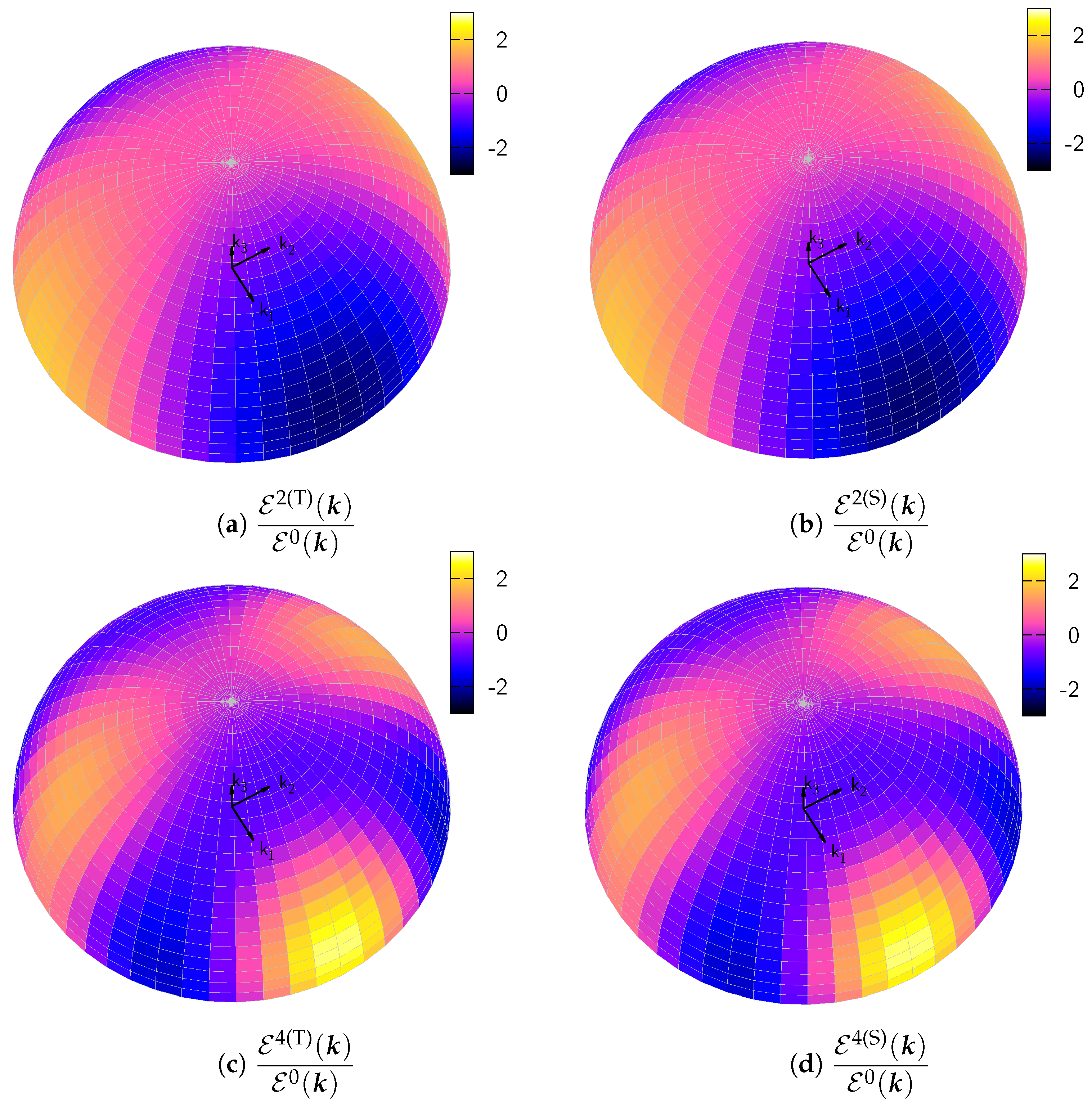
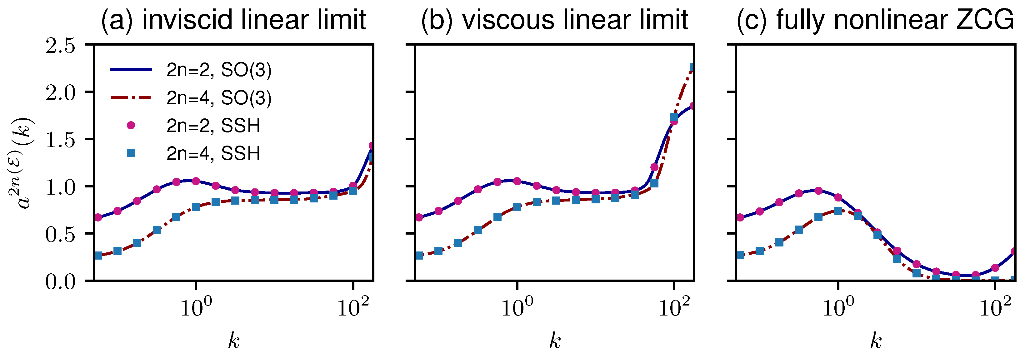
Further, to observe the scale effects of anisotropy in different degrees, we define a normalized spectrum for $\mathcal{E}$ in degree $2n$ as shown below:

$$a^{2n\left(\mathcal{E}\right)}\left(k\right)=\frac{1}{E\left(k\right)}\underset{S_k}{\int \int }\left|{\mathcal{E}}^{2n}\left(\mathit{k}\right)\right|{\mathrm{d}}^2\mathit{k}.$$

(30)

One always obtains 0 if naively removing the absolute value operator $|·|$ from the integrand for any $n>0$. Trivially, we have $a^{0\left(\mathcal{E}\right)}\left(k\right)=1$, and for isotropic turbulence $a^{2n\left(\mathcal{E}\right)}\left(k\right)=0$ for $n>0$. We can roughly regard the directional anisotropy of $\widehat{\mathit{R}}\left(\mathit{k}\right)$ in degree $2n>0$ at k as a negligible component when $a^{2n\left(\mathcal{E}\right)}\left(k\right)\ll 1$; otherwise, it is considerable when $a^{2n\left(\mathcal{E}\right)}\left(k\right)\sim 1$. Figure 5 presents $a^{2n\left(\mathcal{E}\right)}\left(k\right)$ obtained by the SO(3) expansion and the SSH decomposition, respectively, for the maximum destabilization case, at $St=5$, in three different limits. All of the figures indicate that the spherical harmonics decomposition agrees with the tensorial expansion very well with high accuracy in both degree 2 and degree 4, either with or without a nonlinear mechanism, at any length scale.

4.3. Analysis on High-Degree Anisotropy

As introduced before, the dynamics of high-degree anisotropy are of great importance in modeling anisotropic turbulence. The SSH decomposition that can be easily extended to high degrees permits us to explore the generating and damping of high-degree anisotropy in rotating shear flows. To consider the polarization anisotropy, we decompose frame-invariant $\left|Z\right(\mathit{k}\left)\right|$ by the SSH, for $Z\left(\mathit{k}\right)$ cannot be decomposed by spherical harmonics directly since it is singular at the pole. Analogous to (15), one finds

$$\left|Z\left(\mathit{k}\right)\right|=z_0\left(1+\sum _{n=1}^{\infty }\sum _{m=-2n}^{2n}{z}_{2n}^{{}^{\prime }m}\left(k\right)Y_{2n,m}({\theta }_k,{\varphi }_k)\right),$$

(31)

with

$$z_0=\frac{1}{4\pi k^2}\underset{S_k}{\int \int }\left|Z\left(\mathit{k}\right)\right|{\mathrm{d}}^2\mathit{k},$$

(32)

Also, we define

$$Z^{2n}\left(\mathit{k}\right)=\sum _{m=-2n}^{m=2n}{z}_{2n}^{{}^{\prime }m}\left(k\right)Y_{2n}^m({\theta }_k,{\varphi }_k),n=1,2,3\cdots ,$$

(33)

and

$$a^{2n\left(Z\right)}\left(k\right)=\frac{1}{4\pi k^2{z}_0}\underset{S_k}{\int \int }\left|Z^{2n}\left(\mathit{k}\right)\right|{\mathrm{d}}^2\mathit{k}.$$

(34)

The decomposition allows us to obtain high degrees of polarization anisotropy.

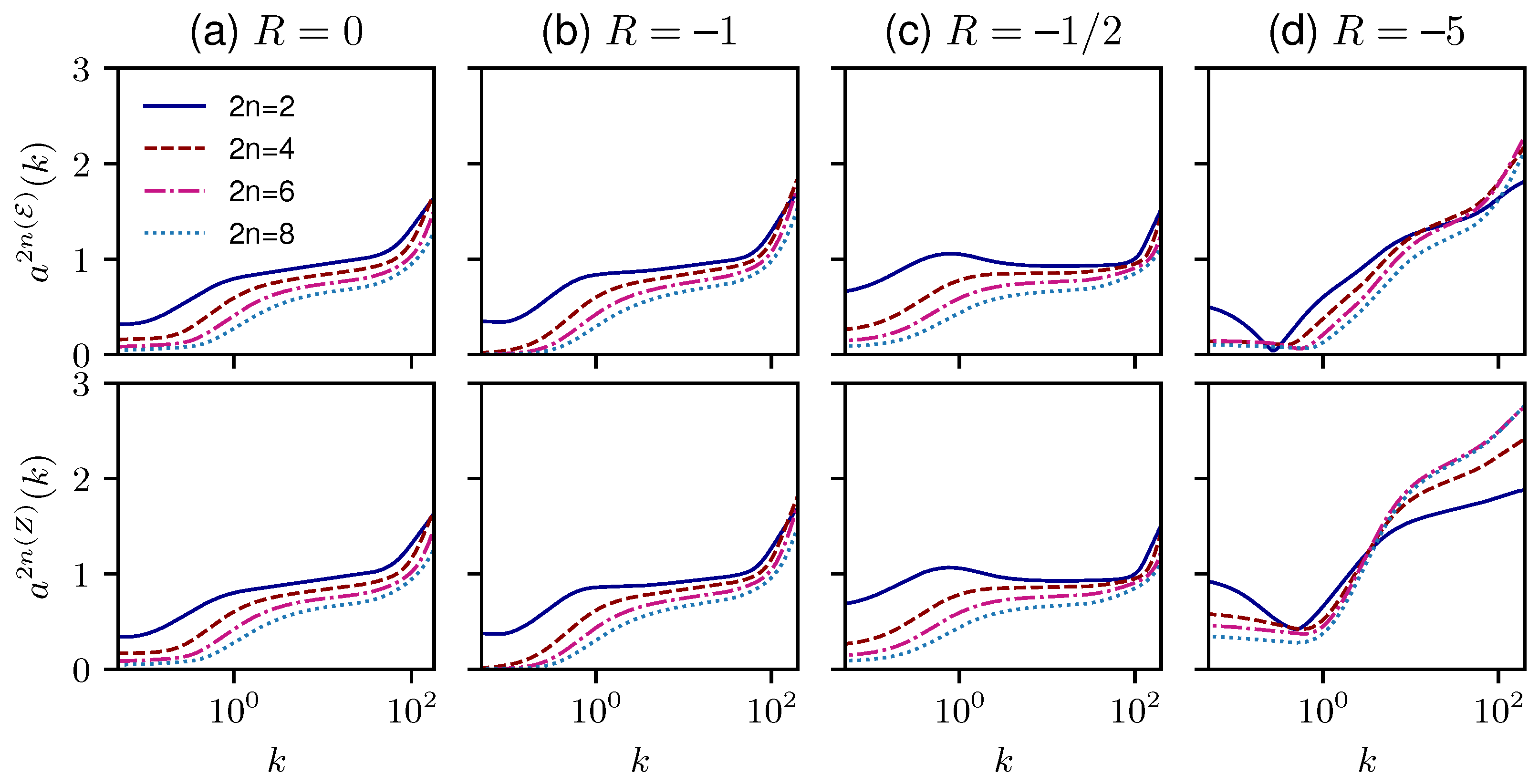
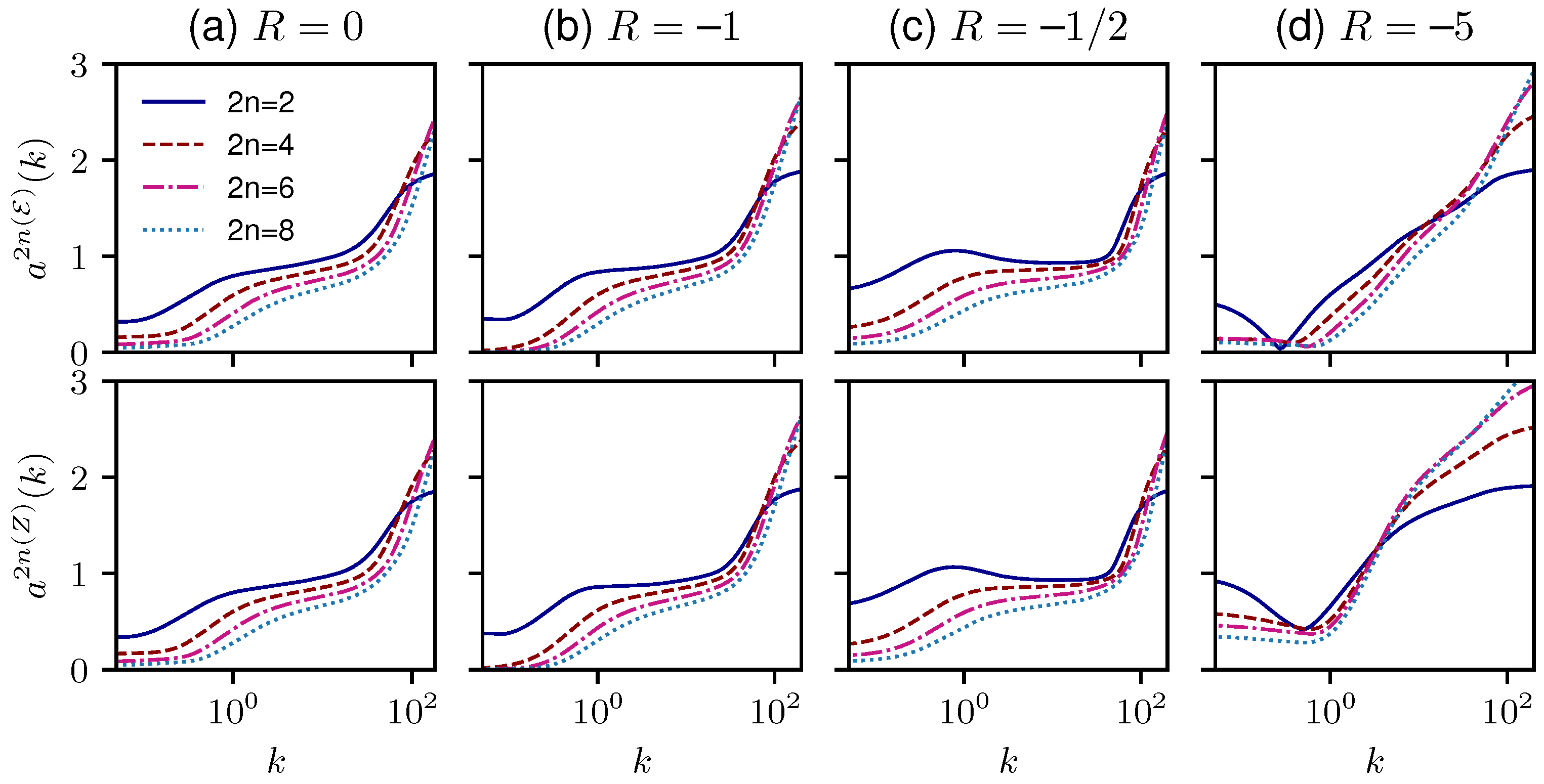
First, we investigate $a^{2n\left(\mathcal{E}\right)}\left(k\right)$ and $a^{2n\left(Z\right)}\left(k\right)$ for $2n=2,4,6,8$ in the inviscid limit (Figure 6) and viscous linear limit (Figure 7), for various values of R, at $St=5$.

Overall, for the same case, the distribution of directional anisotropy in terms of degree and wave number looks similar to its corresponding one for polarization anisotropy. The anisotropy of degree 2 generated by the linear operator dominates in most scale ranges and in all cases. Note that $a^{2n\left(\mathcal{E}\right)}\left(k\right)$ and $a^{2n\left(Z\right)}\left(k\right)$ are the anisotropy divided by the corresponding zero degree values, so they are actually the relative anisotropy in degree $2n$. Accordingly, all the simulations show stronger relative high-degree anisotropy at the largest k’s than at the smallest k’s. Comparing Figure 7 to Figure 6, not surprisingly, we find that the viscosity acts basically in the largest k range (roughly $k>100$), namely, the dissipating scale: the viscosity weakens the anisotropy in degree 2 but enhances other higher-degree components for the largest k values. The stabilizing case contributes the most different behavior, which shows quite small anisotropy around the integral length scale (around $k=1$). In this case, the anisotropy of degree 2 does not dominate in the inertial range (around $k=10$) nor in the dissipation range.

The neologism ‘stropholysis’ was coined by Kassinos and Reynolds in the different context of improved single-point closure models in introducing new tensors with respect to the Reynolds stress tensor, and better modeling the effects of background rotation. In our straightforward spectral analysis, the corresponding effect breaks the mirror symmetry in the polarization term, with a direct impact on the imaginary part of Z only. In the present case of the rotating shear, the dynamical effect of stropholysis is mediated by the term $\mathcal{W}+4\mathbf{\Omega }$ in Equation (22b). Accordingly, the related effect vanishes in the case of maximum destabilization, and it is expected to damp, in average, the polarization term in all other cases.

The ‘stropholysis’ term is the only explicitly different term for all cases with various R and the same mean shear rate S: $\mathcal{W}+4\mathbf{\Omega }=(0,S,0)$ for the pure shear case; $\mathcal{W}+4\mathbf{\Omega }=(0,0,0)$ vanishes in the maximum destabilization case; $\mathcal{W}+4\mathbf{\Omega }=(0,-S,0)$ for the neutral case, with the same net mean vorticity but opposite sign to $R=0$; and $\mathcal{W}+4\mathbf{\Omega }=(0,-9S,0)$ for the stabilizing case $R=-5$ with relatively large net mean vorticity.

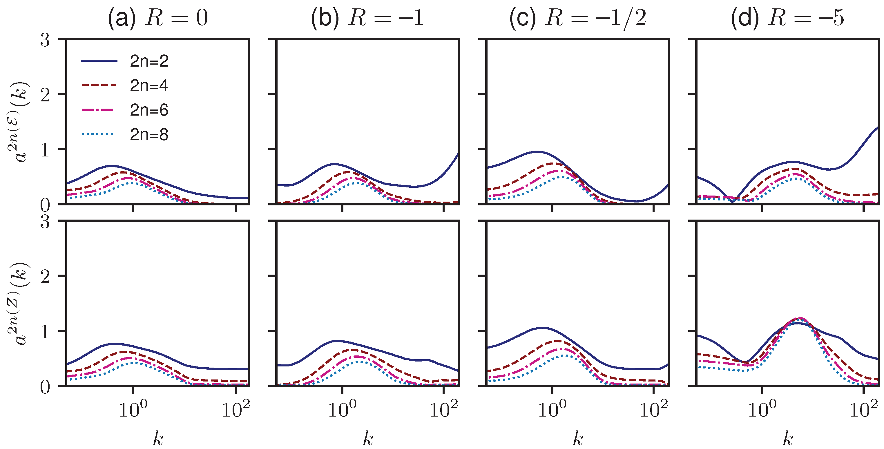
We present in Figure 8 the results obtained by the fully nonlinear ZCG. In all cases, the anisotropy in all the degrees reduces remarkably in the inertial and dissipation ranges, especially for $2n>2$. This indicates that the RTI term used in the ZCG model works efficiently for anisotropy higher than degree 2 as we expected.

5. Towards a More General Decomposition for a Vector Field

This section is motivated by recent studies by Daniel Schertzer, Ioula Chiriginskaia, and coworkers, who mentioned in [30] the following: For instance, it seems ironic that multifractals have been mostly restricted to scalar-valued fields, whereas cascades were first invoked for the wind velocity.

In the past, the important context of internal intermittency and its scaling was mainly investigated using scalar structure functions for moments of velocity increments in physical space. For models developed in spectral space, shell models were essentially restricted to isotropic turbulence.

Recent attempts to describe really anisotropic turbulent flows in terms of vector fields are thereby reviewed in this section. We first address the case of smooth vector fields, with a possible linkage to a modal projection, more complex than the Craya/Herring one, and related expansions in terms of VSHs. In the second part, intermittent vector fields are touched upon with the multifractal approach of Schertzer’s group.

5.1. Using a General Toroidal/Poloidal Decomposition

Meetings around the DFGA theme (dynamics of geophysical and astrophysical fluids) have shown promising and truly multidisciplinary perspectives. For instance, the CNRS International Colloquium—Geophysical and Astrophysical Flows—took an interdisciplinary approach (organized by Philippe Fraunié, on October 16–18, in Paris, France), with several talks that addressed the use of VSH, from smooth to intermittent fields.

Decomposition in terms of VSH (vectorial spherical harmonics) was used by Rieutord (1987) [31] in order to solve linear operators of rotating flow on spheres in physical space. The essential difference with the simplified toroidal/poloidal decomposition in physical space, closely related to that of Craya in Fourier space, is a more complex definition of the toroidal mode as

$${\mathit{u}}^{\left(to\right)}\left(\mathit{r}\right)=\mathbf{\nabla }\times \left(s^{\left(to\right)}\left(\mathit{r}\right)\frac{\mathit{r}}{r}\right),$$

(35)

following Chandrasekkhar (1981) [32]. This amounts to the substitution of the unit radial vector $\mathit{r}/r$ to the polar axis n, and the problem of some singular points on the surface of a sphere is not restricted to the pole of a polar-spherical system of coordinates.

Looking at the decomposition in terms of spherical harmonics, the (new) toroidal mode is expanded as

$${\mathit{u}}^{\left(to\right)}(r,{\theta }_r,{\varphi }_r)=\sum _{n=0}^N\sum _{m=-n}^n{u}_n^m\left(r\right)\mathbf{\nabla }\times \left(Y_n^m({\theta }_r,{\varphi }_r)\frac{\mathit{r}}{r}\right)$$

ref. [31].

On the other hand, the similarity between the representation in physical space and the one in Fourier space is conserved, but the counterpart in Fourier space is no longer purely algebraic. A spectral surrogate of Equation (35) is

$${\widehat{\mathit{u}}}^{\left(to\right)}\left(\mathit{k}\right)=\mathit{k}\times \left(\frac{\partial s^{(to+)}\left(\mathit{k}\right)}{\partial \mathit{k}}\right).$$

(36)

Interestingly, the change of the operator from physical to spectral space is very similar to the one for the advection operator. For the advection term, one has

$$x_n\frac{\partial }{\partial x_m}\to -k_m\frac{\partial }{\partial k_n}$$

As inferred from the new toroidal/poloidal (or spheroidal) modal projection in physical space, from Equation (35), we propose

$$\widehat{\mathit{u}}\left(\mathit{k}\right)=\mathit{\alpha }\times \left(k\frac{\partial }{\partial \mathit{k}}\left(s^{(to+)f}\left(\mathit{k}\right)\right)\right)+\mathit{\alpha }\times \left(\mathit{\alpha }\times \left(k\frac{\partial }{\partial \mathit{k}}\left(s^{(po+)f}\left(\mathit{k}\right)\right)\right)\right),$$

(37)

where a classical SSH decomposition holds for $s^{(to+)}$ and $s^{(po+)}$, with

$$s^{(to+)}\left(\mathit{k}\right)=\sum _{n=0}^N\sum _{m=-n}^n{t}_n^m\left(k\right)Y_n^m({\theta }_k,{\varphi }_k),s^{(po+)}\left(\mathit{k}\right)=\sum _{n=0}^N\sum _{m=-n}^n{p}_n^m\left(k\right)Y_n^m({\theta }_k,{\varphi }_k).$$

(38)

Finally, the helical modes in Equation (6) are expressed as

$${\mathit{u}}_{\mathit{s}}\left(\mathit{k}\right)=\frac{1}{2}\widehat{\mathit{u}}\left(\mathit{k}\right)·\mathit{N}(-\mathit{s}\mathit{\alpha })$$

$$=-\frac{1}{2}\sum _{n=0}^N\sum _{m=-n}^n\left(p_n^m-s𝚤t_n^m\right)\left({\left(Y_n^m\right)}_{,\theta }-s𝚤\frac{1}{sin{\theta }_k}{\left(Y_n^m\right)}_{,\varphi }\right),s=\pm 1.$$

(39)

It is, therefore, possible to reconstruct the spectral tensors from the above-mentioned VSH expansion of the helical modes, but this task is very complex. Looking at the two-point second-order spectral tensor, one can recall that the implicit use of VSH should only concern the polarization term Z.

5.2. Recent Progresses towards Stochastic Fields and Multifractal Approach

With the viewpoint of working with intermittent vector fields, is it possible to use Fourier space beyond the conventional shell models for isotropic turbulence? A first answer was given by Chiriginskaya et al. (1998) [33], from a seminal model by Chiriginskaia and Schertzer (1997) [34], who introduced a cascade of gyroscopes. With respect to the very old analogy of the cascade of eddies as the fragmentation of (scalar) grains, with, for instance, the log-normal distribution inspired by Kolmogorov and Obhukov, this approach is based on a dyadic network of triads of vector interactions between a parent eddy and two children eddies, from the largest scale down to the dissipation (in the molecular sense). Each triad forms a (really, 3D) gyroscope. This is a highly seductive approach, and it is based on the formal analogy of the Euler equation for fluids and the Euler equation for a rigid body as put forward by Arnold. This analogy was perhaps pushed to its best form by Waleffe [5] with his principle of triad instability, where the Euler equations for fluid are expanded in terms of helical modes [4]. Needless to say, it seems to be worthwhile to continue in this direction, as well as to clarify the mutual links with the general approach defining multifractal operators acting on vector fields [33].

6. Conclusions, Perspectives of Turbulence from Earth to Planets, Stars, and Galaxies

The present article, started from seminal studies of Jack Herring for modal projection and expansions in terms of spherical harmonics, is essentially technical. We investigate how to project solenoidal fields, mainly the velocity field, on a reduced number of modes. Projection is systematically carried out in physical space and in spectral one for the fluctuating field(s), with comparison, using 3D, direct and inverse, integral Fourier transform. From a random velocity field (possibly augmented from a buoyancy field and from a magnetic field), corresponding expansions of spectral tensors are derived. For the latter statistical applications, we emphasize the two-point second-order spectral tensor of fluctuating velocity. As far as possible, we emphasize the mathematical treatment of vectors, for instance, using VSH, in addition to SSH for scalar fields. In this sense, the expansion of the second-order spectral tensor $\widehat{\mathbf{R}}$ can directly result from the VSH expansion of $\widehat{\mathit{u}}$ in building ${\widehat{\mathit{u}}}^{\ast }\otimes \widehat{\mathit{u}}$. This possibility is briefly explored in Section 5.1 but appears as a formidable task. On the other hand, the possible underlying vectorial aspect is reduced to only the polarization part Z of the spectral tensor $\widehat{\mathbf{R}}$ since $\mathcal{E}$, $\mathcal{H}$, and even the Z-modulus can be treated as true scalars. Accordingly, a special way of expanding Z is investigated, forcing its correct convergence towards the pole of the system of the polar-spherical system of coordinates, which is puzzling for applying the Craya–Herring projection for non-axisymmetric statistical configurations. The particular example of rotating sheared turbulence is revisited from [6], with new unpublished results, in Section 4. We validate the equivalency of the tensorial SO(3)-type expansion and the SSH decomposition using the data obtained by the ZCG model. The analysis on high-degree anisotropy (higher than in ZCG) is first limited to the linear limit. Also, we verify that the nonlinear terms of the ZCG model damp the high-degree anisotropy efficiently as expected. In addition to the investigation of the anisotropy of the second-order correlations, for quasi-homogeneous turbulence subject to more general mean velocity gradients, the numerical treatment of the convection term by the mean flow in the ZCG model could be applied to DNSs.

New ways for describing intermittent turbulent flows are discussed, using vector fields and thereby going beyond the conventional use of scalar statistics for, for example, structure functions.

Last, but not least, applications to geophysics and astrophysics are expected from the title of the special issue that includes from Earth to planets, stars, and galaxies. To which extent are the above-mentioned technical developments useful for these issues? Some recent reviews are in [10,35]. The mathematical structure of the anisotropic turbulent flows is investigated. Still, their governing equations are hardly shown and discussed, except for rotating shear flows in Section 4, in the presence of body forces and/or basic large-scale flow: such a dynamical aspect is essential for geophysics and astrophysics and is discussed as follows.

6.1. Linear and Quasi-Linear Models from Geophysics to Accretion Discs in Astrophysics

If the linear mechanisms that are responsible for turbulence production and generation of various wave regimes are first investigated, we can move from linear stability analyses to the so-called “rapid distortion theory” and beyond. The rapid evolution of developed turbulence can be investigated in neglecting the explicit nonlinear terms but in initializing turbulence, such as for large Reynolds numbers. Linear responses can be applied to both initial data or to a given force representing nonlinearity as an impulsional response. A modern way towards rather complex inhomogeneous flows is in progress in the ‘resolvent approach’.

The linear dynamics is useful for geophysical and astrophysical flows that are subjected to various dispersive waves: inertial waves in rotating turbulence, gravity waves in stably stratified flows, Alfvén waves in MHD, and various combinations of them. A recent analysis [36] shows, for instance, how destabilizing the resonances are between these waves in an elliptic core.

Application to the dynamics of accretion discs can be started from simple models for quasi-incompressible, quasi-homogeneous sheared turbulence [37], using spatial Fourier harmonics (or mean-flow-advected Fourier modes). In these studies, the nonlinearity is implicit and contributes to the regeneration of active modes, for which the linear mechanisms of non-normal algebraic growth are essential. Additional effects of mean stratification are analyzed in [38].

6.2. Models with Explicit Nonlinearity for Cascades

Wave turbulence theory is a nonlinear theory, even if it is reduced to weak interactions of nonlinear waves (see, e.g., ref. [39] and the references therein). One of the most complete analyses of inertial wave turbulence theory was developed in [40] for the asymptotic dynamics of rotating turbulence. Equations for the fluctuating field and for spectral tensors until the third order were expanded in terms of helical modes, which are the eigenmodes of inertial waves. Close analogies with anisotropic EDQNM, beyond [4], were used. It appears that when the turbulent flow is dominated by dispersive waves, the nonlinearity is drastically reduced and only survives at very large times via the nonlinear resonances of waves. In this asymptotic limit, a quasi-normal assumption, or zero value of cumulants (fourth order if the basic nonlinearity is triadic), becomes exact.

Of course, the cascade process for strong turbulence essentially needs an explicit model of nonlinearity. We mentioned EDQNM (anisotropic multimodal), as for the ZCG model in Section 4. In this case, where the dispersive waves are not dominant, the QN assumption can be a dead end, and ought to be complemented by a QN ingredient, as an empirical damping of fourth-order cumulants. Note that the toroidal mode in stably stratified turbulence is a 3D non-propagating mode, which renders such turbulence outside the scope of conventional wave–turbulence theory. Consequently, a new theory of weak turbulence is in progress for rotating stably stratified flows (Scott and Cambon, just submitted to JFM.)

Some applications to stratified turbulence were carried out with a multi-fractal model, supported by lidar observations [41,42]. Anisotropic scale invariance in atmospheric flows was addressed in [43,44].

References

- Herring, J.R. Approach of axisymmetric turbulence to isotropy. Phys. Fluids 1974, 17, 859–872. [Google Scholar] [CrossRef]
- Riley, J.J.; Metcalfe, R.W.; Weissman, M.A. Direct numerical simulations of homogeneous turbulence in density-stratified fluids. AIP Conf. Proc. 1981, 76, 79–112. [Google Scholar]
- Craya, A. Contribution à l’analyse de la Turbulence Associée à des Vitesses Moyennes. Ph.D. Thesis, Université de Grenoble, Grenoble, France, 1957. [Google Scholar]
- Cambon, C.; Jacquin, L. Spectral approach to non-isotropic turbulence subjected to rotation. J. Fluid Mech. 1989, 202, 295–317. [Google Scholar] [CrossRef]
- Waleffe, F. The nature of triad interactions in homogeneous turbulence. Phys. Fluids A Fluid Dyn. 1992, 4, 350–363. [Google Scholar] [CrossRef]
- Zhu, Y.; Cambon, C.; Godeferd, F.; Salhi, A. Nonlinear spectral model for rotating sheared turbulence. J. Fluid Mech. 2019, 866, 5–32. [Google Scholar] [CrossRef]
- Cambon, C. Multipoint turbulence structure and modelling: The legacy of Antoine Craya. Comptes Rendus Méc. 2017, 345, 627–641. [Google Scholar] [CrossRef]
- Smith, L.M.; Waleffe, F. Generation of slow large scales in forced rotating stratified turbulence. J. Fluid Mech. 2002, 451, 145–168. [Google Scholar] [CrossRef] [Green Version]
- Galmiche, M.; Hunt, J.; Thual, O.; Bonneton, P. Turbulence-mean field interactions and layer formation in a stratified fluid. Eur. J. Mech.-B/Fluids 2001, 20, 577–585. [Google Scholar] [CrossRef]
- Sagaut, P.; Cambon, C. Homogeneous Turbulence Dynamics, 2nd ed.; Springer: Cham, Switzerland, 2018. [Google Scholar] [CrossRef]
- Rubinstein, R.; Kurien, S.; Cambon, C. Scalar and tensor spherical harmonics expansion of the velocity correlation in homogeneous anisotropic turbulence. J. Turbul. 2015, 16, 1058–1075. [Google Scholar] [CrossRef] [Green Version]
- Briard, A.; Iyer, M.; Gomez, T. Anisotropic spectral modeling for unstably stratified homogeneous turbulence. Phys. Rev. Fluids 2017, 2, 044604. [Google Scholar] [CrossRef]
- Cambon, C.; Teissèdre, C.; Jeandel, D. Etude d’effets couplés de rotation et de déformation sur une turbulence homogène. J. Mec. Theor. Appl. 1985, 5, 629. [Google Scholar]
- Zhu, Y. Modelling and Calculation for Shear-Driven Rotating Turbulence, with Multiscale and Directional Approach. Ph.D. Thesis, Université de Lyon, Lyon, France, 2019. [Google Scholar]
- Batchelor, G.; Proudman, I. The effect of rapid distortion of a fluid in turbulent motion. Q. J. Mech. Appl. Math. 1954, 7, 83–103. [Google Scholar] [CrossRef]
- Salhi, A.; Cambon, C. An analysis of rotating shear flow using linear theory and DNS and LES results. J. Fluid Mech. 1997, 347, 171–195. [Google Scholar] [CrossRef]
- Kassinos, S.C.; Reynolds, W.C.; Rogers, M.M. One-point turbulence structure tensors. J. Fluid Mech. 2001, 428, 213–248. [Google Scholar] [CrossRef]
- Orszag, S.A. Analytical theories of turbulence. J. Fluid Mech. 1969, 41, 363–386. [Google Scholar] [CrossRef]
- Cambon, C.; Mons, V.; Gréa, B.J.; Rubinstein, R. Anisotropic triadic closures for shear-driven and buoyancy-driven turbulent flows. Comput. Fluids 2017, 151, 73–84. [Google Scholar] [CrossRef]
- Burlot, A.; Gréa, B.J.; Godeferd, F.S.; Cambon, C.; Griffond, J. Spectral modelling of high Reynolds number unstably stratified homogeneous turbulence. J. Fluid Mech. 2015, 765, 17–44. [Google Scholar] [CrossRef]
- Mons, V.; Cambon, C.; Sagaut, P. A spectral model for homogeneous shear-driven anisotropic turbulence in terms of spherically averaged descriptors. J. Fluid Mech. 2016, 788, 147–182. [Google Scholar] [CrossRef] [Green Version]
- Weinstock, J. Theory of the pressure–strain rate. Part 2. Diagonal elements. J. Fluid Mech. 1982, 116, 1–29. [Google Scholar] [CrossRef]
- Weinstock, J. Analytical theory of homogeneous mean shear turbulence. J. Fluid Mech. 2013, 727, 256–281. [Google Scholar] [CrossRef]
- Rogallo, R.S. Numerical Experiments in Homogeneous Turbulence. NASA STI/Recon Tech. Rep. N 1981, 81, 31508. [Google Scholar]
- Lesur, G.; Longaretti, P.Y. On the relevance of subcritical hydrodynamic turbulence to accretion disk transport. Astron. Astrophys. 2005, 444, 25–44. [Google Scholar] [CrossRef]
- Hanazaki, H.; Hunt, J.C.R. Structure of unsteady stably stratified turbulence with mean shear. J. Fluid Mech. 2004, 507, 1–42. [Google Scholar] [CrossRef] [Green Version]
- Salhi, A.; Cambon, C. Stability of rotating stratified shear flow: An analytical study. Phys. Rev. E 2010, 81, 026302. [Google Scholar] [CrossRef] [Green Version]
- Bradshaw, P. The analogy between streamline curvature and buoyancy in turbulent shear flow. J. Fluid Mech. 1969, 36, 177–191. [Google Scholar] [CrossRef]
- Salhi, A.; Jacobitz, F.G.; Schneider, K.; Cambon, C. Nonlinear dynamics and anisotropic structure of rotating sheared turbulence. Phys. Rev. E 2014, 89, 013020. [Google Scholar] [CrossRef] [Green Version]
- Schertzer, D.; Tchiguirinskaia, I. A century of turbulent cascades and the emergence of multifractal operators. Earth Space Sci. 2020, 7, e2019EA000608. [Google Scholar] [CrossRef] [Green Version]
- Rieutord, M. Linear theory of rotating fluids using spherical harmonics part I: Steady flows. Geophys. Astrophys. Fluid Dyn. 1987, 39, 163–182. [Google Scholar] [CrossRef]
- Chandrasekhar, S. Hydrodynamic and Hydromagnetic Stability; Dover Publications: New York, USA, 1981. [Google Scholar]
- Chigirinskaya, Y.; Schertzer, D.; Lovejoy, S. An alternative to shell-models: More complete and yet simple models of intermittency. In Proceedings of the Advances in Turbulence VII: Proceedings of the Seventh European Turbulence Conference, Saint-Jean Cap Ferrat, France, 30 June–3 July 1998; pp. 263–266. [Google Scholar]
- Chigirinskaya, Y.; Schertzer, D. Cascade of Scaling Gyroscopes: Lie Structure, Universal Multifractals and Self-Organized Criticality in Turbulence. In Stochastic Models in Geosystems; Molchanov, S.A., Woyczynski, W.A., Eds.; Springer: New York, NY, USA, 1997; pp. 57–81. [Google Scholar] [CrossRef]
- Cambon, C.; Laguna, A.A.; Zhou, Y. CFD for turbulence: From fundamentals to geophysics and astrophysics. Comptes Rendus Méc. 2022, 350, 1–20. [Google Scholar] [CrossRef]
- Salhi, A.; Cambon, C. Magneto-gravity-elliptic instability. J. Fluid Mech. 2023, 963, A9. [Google Scholar] [CrossRef]
- Chagelishvili, G.; Zahn, J.P.; Tevzadze, A.; Lominadze, J. On hydrodynamic shear turbulence in Keplerian disks: Via transient growth to bypass transition. Astron. Astrophys. 2003, 402, 401–407. [Google Scholar] [CrossRef] [Green Version]
- Salhi, A.; Lehner, T.; Godeferd, F.; Cambon, C. Wave–vortex mode coupling in astrophysical accretion disks under combined radial and vertical stratification. Astrophys. J. 2013, 771, 103. [Google Scholar] [CrossRef] [Green Version]
- Nazarenko, S. Wave Turbulence; Springer Science & Business Media: Berlin/Heidelberg, Germany, 2011; Volume 825. [Google Scholar]
- Bellet, F.; Godeferd, F.; Scott, J.; Cambon, C. Wave turbulence in rapidly rotating flows. J. Fluid Mech. 2006, 562, 83–121. [Google Scholar] [CrossRef]
- Radkevich, A.; Lovejoy, S.; Strawbridge, K.; Schertzer, D. The elliptical dimension of space-time atmospheric stratification of passive admixtures using lidar data. Phys. A Stat. Mech. Its Appl. 2007, 382, 597–615. [Google Scholar] [CrossRef]
- Lilley, M.; Lovejoy, S.; Strawbridge, K.; Schertzer, D. 23/9 dimensional anisotropic scaling of passive admixtures using lidar data of aerosols. Phys. Rev. E 2004, 70, 036307. [Google Scholar] [CrossRef] [PubMed] [Green Version]
- Lewis, G.; Lovejoy, S.; Schertzer, D.; Pecknold, S. The scale invariant generator technique for quantifying anisotropic scale invariance. Comput. Geosci. 1999, 25, 963–978. [Google Scholar] [CrossRef]
- Lazarev, A.; Schertzer, D.; Lovejoy, S.; Chigirinskaya, Y. Unified multifractal atmospheric dynamics tested in the tropics: Part II, vertical scaling and generalized scale invariance. Nonlinear Process. Geophys. 1994, 1, 115–123. [Google Scholar] [CrossRef] [Green Version]
Figure 1.
Craya–Herring frame of reference.
Figure 2.
Time evolution of turbulent kinetic energy. Comparisons of results from the cases with typical values of R: (a) in the inviscid linear limit; (b) in the viscous linear limit; and (c) with fully nonlinear ZCG.
Figure 3.
Time evolution of the deviatoric part of the Reynolds stress tensor . Comparisons of results from the cases with typical values of R: (a) in inviscid linear limit; (b) in viscous linear limit; and (c) with fully nonlinear ZCG.
Figure 4.
Spherical distributions of and in viscous linear limit with at at the wavenumber . Comparison of results obtained by the SO(3)-type expansion and SSH decomposition, respectively.
Figure 5.
Spherically averaged anisotropy spectra for in degree and at . Comparisons of the results obtained respectively by tensorial expansion (SO(3) type) and SSH decomposition: (a) in the inviscid linear limit; (b) in the viscous linear limit; and (c) with fully nonlinear ZCG.
Figure 6.
Spherically integral anisotropy for (top) and for Z (bottom) in degree , in inviscid linear limit at for various values of R.
Figure 7.
Spherically integral anisotropy for (top) and for Z (bottom) in degree , in viscous linear limit at for various values of R.
Figure 8.
Spherically integral anisotropy for (top) and for Z (bottom) in degree , with fully nonlinear ZCG, at for various values of R.
Disclaimer/Publisher’s Note: The statements, opinions and data contained in all publications are solely those of the individual author(s) and contributor(s) and not of MDPI and/or the editor(s). MDPI and/or the editor(s) disclaim responsibility for any injury to people or property resulting from any ideas, methods, instructions or products referred to in the content. |
© 2023 by the authors. Licensee MDPI, Basel, Switzerland. This article is an open access article distributed under the terms and conditions of the Creative Commons Attribution (CC BY) license (https://creativecommons.org/licenses/by/4.0/).
Share and Cite
MDPI and ACS Style
Zhu, Y.; Cambon, C. Modal Projection for Quasi-Homogeneous Anisotropic Turbulence. Atmosphere 2023, 14, 1215. https://doi.org/10.3390/atmos14081215
AMA Style
Zhu Y, Cambon C. Modal Projection for Quasi-Homogeneous Anisotropic Turbulence. Atmosphere. 2023; 14(8):1215. https://doi.org/10.3390/atmos14081215
Chicago/Turabian StyleZhu, Ying, and Claude Cambon. 2023. "Modal Projection for Quasi-Homogeneous Anisotropic Turbulence" Atmosphere 14, no. 8: 1215. https://doi.org/10.3390/atmos14081215
Note that from the first issue of 2016, this journal uses article numbers instead of page numbers. See further details here.