Article

Velocity Fluctuations Spectra in Experimental Data on Rayleigh–Taylor Mixing

by
Kurt C. Williams
and
Snezhana I. Abarzhi
*
Department of Mathematics and Statistics, The University of Western Australia, Crawley, Perth, WA 6009, Australia
*
Author to whom correspondence should be addressed.
Atmosphere 2023, 14(7), 1178; https://doi.org/10.3390/atmos14071178
Submission received: 8 June 2023 / Revised: 12 July 2023 / Accepted: 18 July 2023 / Published: 21 July 2023

Abstract

:
Rayleigh–Taylor (RT) interfacial mixing plays an important role in nature and technology, including atmospheric flows. In this work, we identify the physics properties of Rayleigh–Taylor mixing through the analysis of unprocessed experimental data. We consider the fluctuations spectra of the specific kinetic energy of each of the velocity components, and identify their spectral shapes, by employing the group theory guided foundations and the rigorous statistical method. We find the spectral shape parameters, including their mean values and relative errors, and apply the Anderson–Darling test to inspect the residuals and the goodness-of-fit. We scrupulously study the effect of the fitting window and identify, for each velocity component, the best fit interval, where the relative errors are small and the goodness of fit is excellent. We reveal that the fluctuations spectra in RT mixing experiments can be described by a compound function, being a product of a power-law and an exponential. The data analysis results unambiguously discovered the dynamic anisotropy and the dynamic bias of RT mixing and displayed the necessity to improve the design of experiments on RT mixing.

1. Introduction

This paper was invited to contribute to Turbulence from Earth to Planets, Stars and Galaxies, the Commemorative Issue Dedicated to the Memory of Jackson Rae Herring, of the Atmosphere. Dr. Jackson Herring provided very important contributions to our understanding and modeling of realistic turbulent processes. This may include his earlier works on the growth of uncertainty in decaying isotopic turbulence [1], the decay of two-dimensional homogeneous turbulence [2], and the strain-based Lagrangian-history turbulence theory [3]. This may also include his later investigations of the Lagrangian velocity correlations in homogeneous isotropic turbulence [4] and the far-dissipation range of turbulence studies of [5]. The research interests of Dr. Jackson Herring ranged broadly, from the use and testing of closures in fluid turbulence, such as the Prandtl number dependence of Nusselt number in direct numerical simulations [6], to the issues and problems of stably stratified turbulence [7].
In as much as turbulence is considered to be the last unsolved problem of classical physics, Rayleigh–Taylor interfacial mixing are its more complex counterparts [8]. To better understand self-similar Rayleigh–Taylor mixing, bias free interpretation of data is necessary [8,9,10,11]. Our work yields physics properties and anomalous scaling of Rayleigh–Taylor mixing and identifies directions for advancements in experimental design based on analysis of experimental data [12]. We are inspired by approaches developed by colleagues [3,7,13,14,15,16,17].
Rayleigh–Taylor instability (RTI) is a hydrodynamic instability that develops at the interface between fluids of differing densities that are accelerated against their density gradients [18,19]. First investigated by Lord Rayleigh in 1883, RTI is an ubiquitous element of many natural and engineered processes. Of particular interest to modern science is the nature of late-stage interfacial Rayleigh–Taylor (RT) mixing. The myriad of potential factors and expected dynamics means that a bias-free, statistically sound method of data analysis is needed to appreciate the full dynamical picture of RT mixing.
In the natural world, RT mixing is a critical factor for phenomena at a huge disparity of scales, from microscopic to stellar scales. It is responsible for the fingering of interstellar media in the matter pulled along the edges of black holes, and the accelerated ejection matter in both core-collapse supernovae and solar flares. On the Earth, RT mixing is observed in polar deep ocean convection currents, undersea volcano formation, the dispersion of pollutants in the atmosphere, and in coastal boundary up-welling systems in the ocean. In the industrial world, nano-fabrication, fossil fuel extraction, plasma fusion and premixed combustion all exhibit interfacial RT mixing [8,9,11,17,20,21,22,23].
The late-stage of RT dynamics, interfacial RT mixing, is a continuing subject of active research in contemporary science, mathematics, and engineering. RT mixing is uniquely challenging to understand, as it exhibits incredibly complex behaviors and coupling of scales. It is purported that interfacial RT mixing is self-similar, with the length-scale in the acceleration direction growing quadratic with time. However, RT mixing remains a phenomenon of incredibly complex, rich dynamics, evading accurate capture by simplistic models [9,24].
In this work, we employ a rigorous data analysis method, guided by group theory, to analyze the spectral behavior of an RT mixing experiment [12]. We consider the fluctuations of the specific kinetic energy of each of three velocity components. We found that the experimental data revealed properties of RT mixing in good agreement with group theory results. The dynamics observed in experiments exhibit dynamic anisotropy and the dynamic bias of self-similar RT mixing [12], and reveal the necessity of improving the design of experiments on RT mixing [8,10].
The need for statistically rigorous data analysis is borne out of the extreme challenge that RTI, and, in particular, RT mixing, presents to theory, simulations and experiments. Experiments must contend with the vast array of scales that are significant to the dynamics, and must tightly control the implementation of the flow, since even microscopic deviations from the idealized case may rapidly grow into structures and deformations at later times. Furthermore, the need for both highly precise and non-invasive diagnostics further restricts the efficacy of experiments, upon which, for example, numerical simulations are highly dependent for low-level subgrid assumptions [8,9,11,24].
To combat these difficulties, and advance understanding of RT mixing, rigorous data analysis is required [25,25]. Substantial success has recently been achieved, with the data analysis method employed in this paper characterizing the fluctuations spectra of specific kinetic energy, density and mass flux in the direction of the acceleration for an RTI experiment, which has evaded theory analysis for some time due to the inhomogeneity in the fluid densities [26,27,28]. Careful data analysis found excellent agreement with the group theory predictions [28]. It was also consistent with the group theory discovery that RT mixing can keep order and, in fact, retain memory of deterministic conditions, even at late times [9,24,28,29].
For isotropic homogeneous turbulence, accurate quantification of fluctuations spectra in experiments and observations led to the discovery of anomalous scaling. Anomalous scaling is the generic name for departures of the fluctuations spectra in realistic turbulent processes from the canonical Kolmogorov’s scaling laws [13,17,30,31]. Such anomalies are also observed in turbulent boundary layers, passive scalar mixing, buoyancy-driven turbulence, turbulent convection, and compressible turbulence. The classical works find that, in realistic turbulent processes, the spectral shapes of the fluctuations can be more complex than Kolmogorov’s spectra [13,15,16,32,33]. As a function of the mode number, the spectral shape can have a distinct power-law dependence, can be described by a product of a power-law and an exponential, and can also be expressed by a stretched exponential function. Models, including anomalous scaling, accurately capture the properties of fluctuations in experiments and observations. They assert that Kolmogorov turbulence, as an ideal stochastic process, can be an extreme challenge to implement in realistic environments [13,17,25,34,35].
In this work, we investigate data on fluctuations in self-similar RT mixing in the experiments [12,25]. The data are obtained through hot-three-wire anemometry probing. We analyze the fluctuations of the specific kinetic energy of the three velocity components. We employ and further develop the method [25] to identify, with statistical confidence, the spectral shapes of the fluctuations of each of the following three quantities: the mean values of the spectral shape’s parameters, their relative errors, and the goodness of fit. To inspect the residuals, which should be χ 2 2 distributed, the Anderson–Darling test is employed [36]. We find the domains of the mode numbers, where the relative errors of the spectral shape parameters are small and the goodness of fit is excellent. The data analysis unambiguously identifies the dynamic anisotropy, specificity, and heterogeneity, and the dynamic bias, of RT mixing in the experiments [12]. Group theory is employed to explain these properties quantitatively and qualitatively, and to link them to other experiments on RT mixing and realistic turbulent processes [9,16,17,24,32,33,37,38,39]. Our results demonstrate the need for improvements in experimental design for studies in RT mixing, and may help chart directions for future research [8,10,11,24,40,41].

2. Methodology and Foundations

2.1. Theory

2.1.1. Group Theory Methodology

Rayleigh–Taylor dynamics is governed by equations in the bulk, a boundary value problem and an initial value problem. The equations in the bulk of each fluid are the laws of conservation of mass, momentum and energy. They are nonlinear partial differential equations in three-dimensional space and time, and are the Euler equations in the case of ideal fluids. The equation of state closes the system of equations. The singular boundary value problem consists of the boundary conditions at the nonlinear freely evolving unstable fluid interface. These conditions are represented by a sub-set of non-linear partial differential equations. For ideal fluids, the mass flux, the normal component of velocity and the pressure are continuous at the interface, whereas the tangential component of velocity and the specific enthalpy may have a discontinuity. The boundary value problem is also augmented with the boundary conditions at the outside boundaries of the domain. The ill-posed initial value problem is represented by initial perturbations of the interfaces and the flow fields [9,26,42].
The theoretical problem of Rayleigh–Taylor dynamics is intellectually challenging. Success in solving the problem is achieved with the group theory approach, including accurate analytical solutions for the scale-dependent early-time and late-time nonlinear dynamics, as well as for the self-similar Rayleigh–Taylor mixing in a broad range of conditions. Particularly, the dynamics of Rayleigh–Taylor mixing can be captured within the framework of the momentum model that has the same symmetries and scaling transformations as, and is directly linked to, the governing equation [9,24,26,29,43,44,45,46].
Particularly, RT dynamics is driven by a specific, per unit mass, balance of the rate of momentum gain μ ˜ and the rate of momentum loss μ . The gain and loss of specific momentum are associated with the gain ϵ ˜ and dissipation ϵ of the specific energy as μ ˜ = ϵ ˜ / v and μ = ϵ / v , where v is the velocity of the parcel of fluid in the acceleration direction. For constant acceleration with the magnitude g, the rate of momentum loss is μ = C v 2 / L and the rate of energy dissipation is ϵ = C v 3 / L , where C is the drag value and L is the length scale. The rates of gain of momentum and energy are μ ˜ g and ϵ ˜ g v . In the regime of self-similar mixing, the length scale is L | h | , where h is the amplitude in the acceleration direction increasing quadratic with time | h | g t 2 . The rates of loss and gain of momentum relate as μ μ ˜ g , whereas the rates of energy dissipation and gain are time-dependent with ϵ ϵ ˜ g 2 t [9,24,26,29,43,44,45,46].

2.1.2. Scaling Laws and Sensitivity to Deterministic Conditions

In RT mixing, the invariant form of the scaling transformation is the rate of loss of specific momentum μ v 2 / L v l 2 / l , where v ( v l ) is the velocity scale at large (small) length scale L ( l ) . This leads to the velocity scaling v l / v ( l / L ) 1 / 2 , the Reynolds number R e g 2 t 3 / ν , the viscous scale l ν ( ν 2 / μ ) 1 / 3 and the span of scales L / l ν R e 2 / 3 , where L g t 2 and ν is the kinematic viscosity.
These properties depart from those of canonical Kolmogorov turbulence [9,29,34,35,42,43]. Furthermore, in contrast to stochastic canonical turbulence, Rayleigh–Taylor mixing is sensitive to deterministic (initial and flow) conditions [9,24,26,29,42].
To evaluate the sensitivity of fluctuations induced by the RT mixing process to those set by the deterministic conditions, we consider two parcels of fluid involved in the flow with a time delay τ ˜ one after another. The invariance of the rate of momentum loss μ v 2 / L leads to ballistic dynamics, v μ t . The process-induced velocity fluctuations, ∼ μ τ ˜ , are comparable to the fluctuations set deterministically by the parcels’ relative velocities, ∼ ( μ ˜ μ ) τ ˜ . The ratio of the velocity fluctuations and the mean velocity decays with time, ∼ ( τ ˜ / t ) . This suggests that RT mixing can re-laminarize, akin to accelerated turbulent flows [15,24,29,37].

2.1.3. Fluctuations Spectra

In Rayleigh–Taylor mixing, [26,27,29] the invariance of the rate of momentum loss leads the fluctuations of the specific kinetic energy v 2 and the spectral density E ( k )
v 2 E ( k ) d k μ k 2 d k , E ( k ) μ k 2 .
Since RT dynamics is anisotropic, the dynamics in the direction of the acceleration can differ from those in the normal plane. Particularly, while in the mixing regime, the vertical length scale can change self-similarly, h g t 2 , and the horizontal scale can remain nearly invariable, λ c o n s t . In addition to the invariant quantity μ , the fluctuations of the specific kinetic energy corresponding to the velocity components v 2 in the direction normal to the acceleration can be driven by the velocity scale g λ . This leads to
v 2 E ( k ) d k ( g λ ) k 1 d k , E ( k ) g λ k 1 .
In the experiments, [12], due to sensitivity of RT dynamics to deterministic conditions, the fluctuations of the specific kinetic energy corresponding to the velocity components v 2 in the directions normal to the acceleration can also be driven by the velocity scale U ^ . Here, U ^ o ( U ) , with U being the velocity of the co-flowing streams. The scale U ^ is set by the accuracy of the velocity U, being the deterministic noise; which is within a few percent in the experiments [12]. This provides:
v 2 E ( k ) d k U ^ 2 k 1 d k , E ( k ) U ^ 2 k 1 .
Finally, in the experiments [12], the fluctuations of the specific kinetic energy corresponding to the velocity components v 2 can also be driven by the interplay of the velocity scale U ^ and the rate of momentum loss μ g , as
v 2 E ( k ) d k U ^ μ k 3 / 2 d k , E ( k ) U ^ μ k 3 / 2 .
The spectral density in Equation (4) is the geometric mean of the spectral densities of the kinetic energy velocity components, along with, and normal to, the acceleration in Equations (2) and (3), with U ˜ μ k 3 / 2 = ( μ k 2 ) ( U ^ 2 k 1 ) .

2.1.4. Spectral Shapes in Experiments

Quantification of power-laws is a key objective of experimental diagnostics of canonical turbulence and RT mixing. Reliable identification of an exponent and a prefactor of a power-law requires a substantial span of resolved scales; it is a challenge to achieve this in experiments and simulations [10,15,26,41,42,45,46].
In this work, in order to analyze unprocessed raw data from the hot-three-wire anemometry measurements of Rayleigh–Taylor mixing experiments [12,25], and to identify the data-based properties of RT mixing, we apply a compound function represented by a product of a power-law and an exponential
E ( k ) k α exp ( β k )
The compound function E ( k ) k α exp ( β k ) behaves as a power-law for scales k k ν and as an exponential for scales k ν , where k ν is the wave-vector corresponding to the viscous scale, with k ν 1 / l ν . The signs of spectral shape parameters are α , β < 0 , because, in RT mixing with constant acceleration, larger velocities correspond to larger length scales. The use of the compound function in RT spectra is discussed in detail in our earlier works [25,28,28]. The compound function E ( k ) k α exp ( β k ) is applied in turbulence to describe realistic spectra in experiments and observations [9,13,14,16,17,25,30,31,32].

2.2. Outline of Experiments

In this work, we analyze data in the experiments [12] to further understand the properties of RT mixing. Our earlier works studied the fluctuations of the cross-stream velocity component, the density and the mass flux [25,28]. Here we analyze the fluctuations of each of three velocity components. We consider data from the pure Rayleigh–Taylor setup A1S0 and we focus on data taken at very late times to ensure that the RT flow reaches the self-similar mixing [12]. The Reynolds number of the mixing flow is estimated to be ∼ 3.4 × 10 4 [12].
The details of the experiments, the experimental setups, the diagnostics and the data can be found in the works [12,25,28,28].

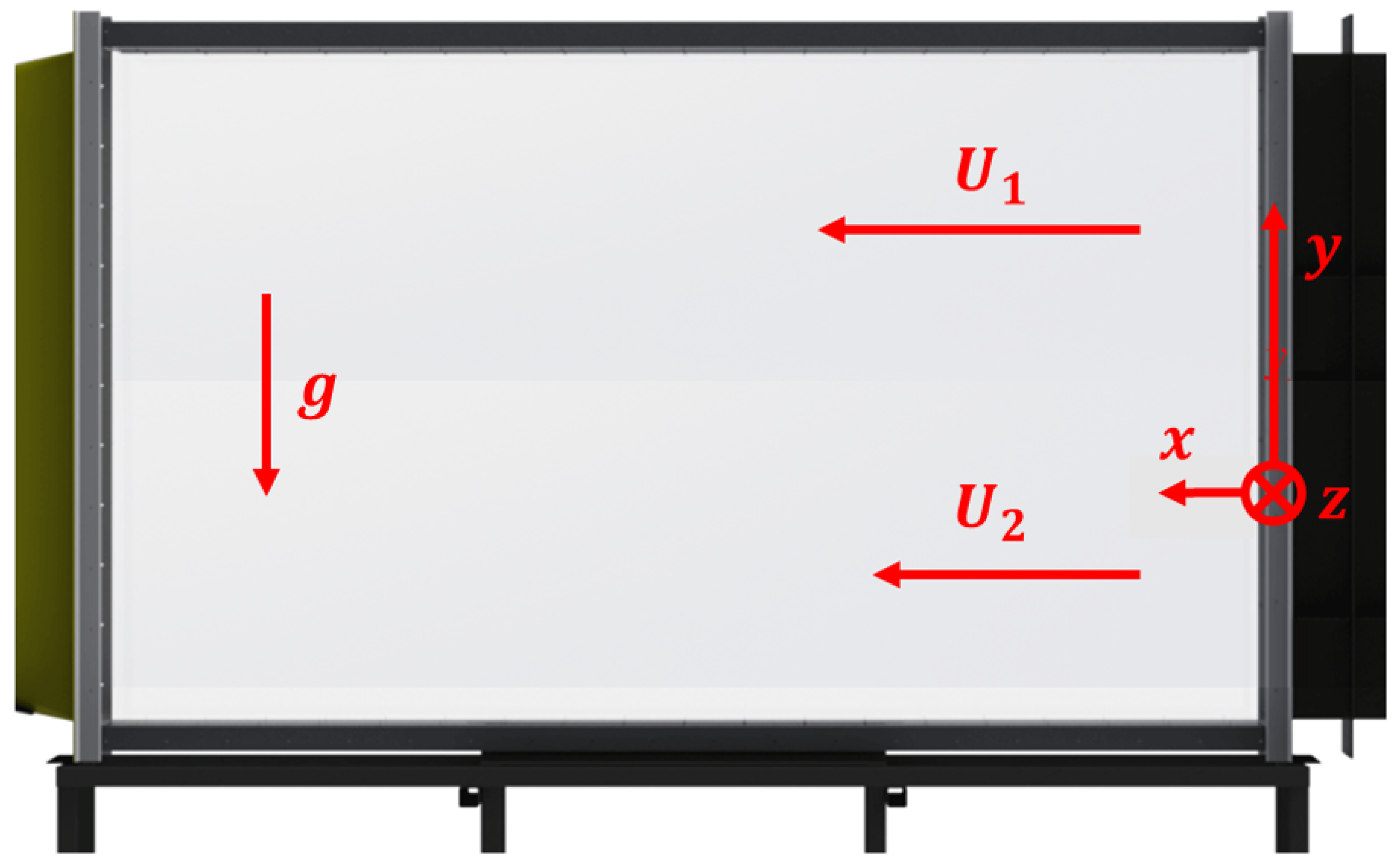
2.2.1. Experimental Setup

For the purpose of completeness and the reader’s convenience, Figure 1 illustrates the schematics of the experiments [12]. The flow is three-dimensional, with the ( x , y , z ) spatial directions and with the ( u , v , w ) corresponding velocity components. In the pure RT setup A1S0, the velocities of the co-flowing streams equal one another, U = U 1 = U 2 , within a few percent accuracy [12].
In Figure 1, as in the experiments [12], the x-direction is the direction of the co-flowing streams. In the x-direction, the velocity component is u. We call it the stream-wise velocity. The y-direction is the direction of the acceleration, which is the Earth’s gravity, and is directed from the heavy (top) to the light (bottom) fluid. In the y-direction, the velocity component is v. We call it cross-stream velocity. The z-direction is normal to the directions of the acceleration and the co-flowing streams. In the z-direction, the velocity component is w. We call it cross-tank velocity [28].

2.2.2. Characteristic Scales in the Experiments

Based on the experimental parameters in the setup A1S0 [12], we evaluated the wave-vector k ν = ( g / ν 2 ) 1 / 3 as k ν = ( 1.13 1.08 ) × 10 3 [ m 1 ] , and the viscous length scale l ν = 2 π / k ν as l ν = ( 5.58 5.84 ) × 10 3 [m]. The scales k ν and l ν were comparable to those of the mode of fastest growth in RTI.
We evaluated the scales which were set by the deterministic noise; particularly, by the 1 % accuracy in the magnitude of the velocity of the co-flowing streams U ^ = 0.01 U = 6.30 × 10 3 [m/s], where U = U 1 = U 2 = 6.3 × 10 1 [m/s]. This yielded the wave-vector k ^ ν = U ^ / ν = ( 4.06 3.79 ) × 10 2 [ m 1 ] and the corresponding length scale λ ^ ν = 2 π / k ^ ν = ( 1.55 1.65 ) × 10 2 [m].
We evaluated the scales which were set by the velocity of the co-flowing streams with magnitude U = U 1 = U 2 = 6.3 × 10 1 [m/s]. This included the wave-vector k ˇ ν = U / ν = ( 4.06 3.79 ) × 10 4 [ m 1 ] , the corresponding length scale λ ˇ ν = 2 π / k ˇ ν = ( 1.55 1.66 ) × 10 4 [m], and the corresponding time scale τ ˇ ν = ν / U 2 = ( 3.91 4.18 ) × 10 5 [s].
The largest horizontal length scale and vertical length scale corresponded to L = 31.5 [m] and H = 1.2 [m], respectively. In this data set, the total sampling time was T = 5 × 10 1 [s]. The horizontal length-scale L and the total sampling time T related as L = U T . The scale H was the tunnel width and it was used to scale the lengths [12].
For further details, including the resolution and the level of instrumental noise, the reader is referred to the works [25,28,28].

2.3. Method of Data Analysis

The data analysis method we employed was successfully applied in [28], predicated on an earlier method in [25,25].
The method is derived from the statistically sound Whittle Maximum Likelihood Estimation (MLE) technique but includes an Anderson–Darling test applying a newly calculated test statistic. The method finds estimations of the model parameters, verifies the goodness of fit and probes the effect of the range of wave-vectors on the estimation values and statistical uncertainty in the fit parameters. By interrogating the effect of the wave-vector range, it is possible to identify the most-likely parameters, the uncertainty in the estimation, and the wave-vector range the model is valid for.

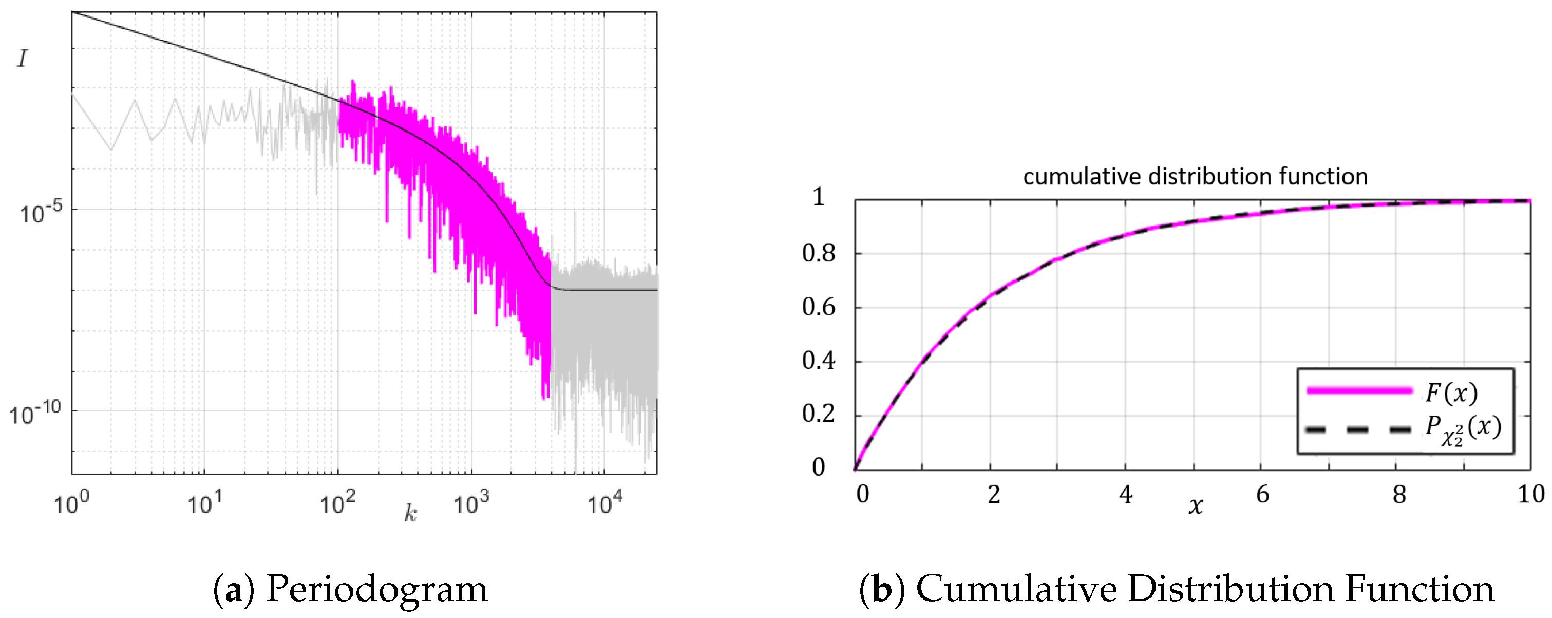
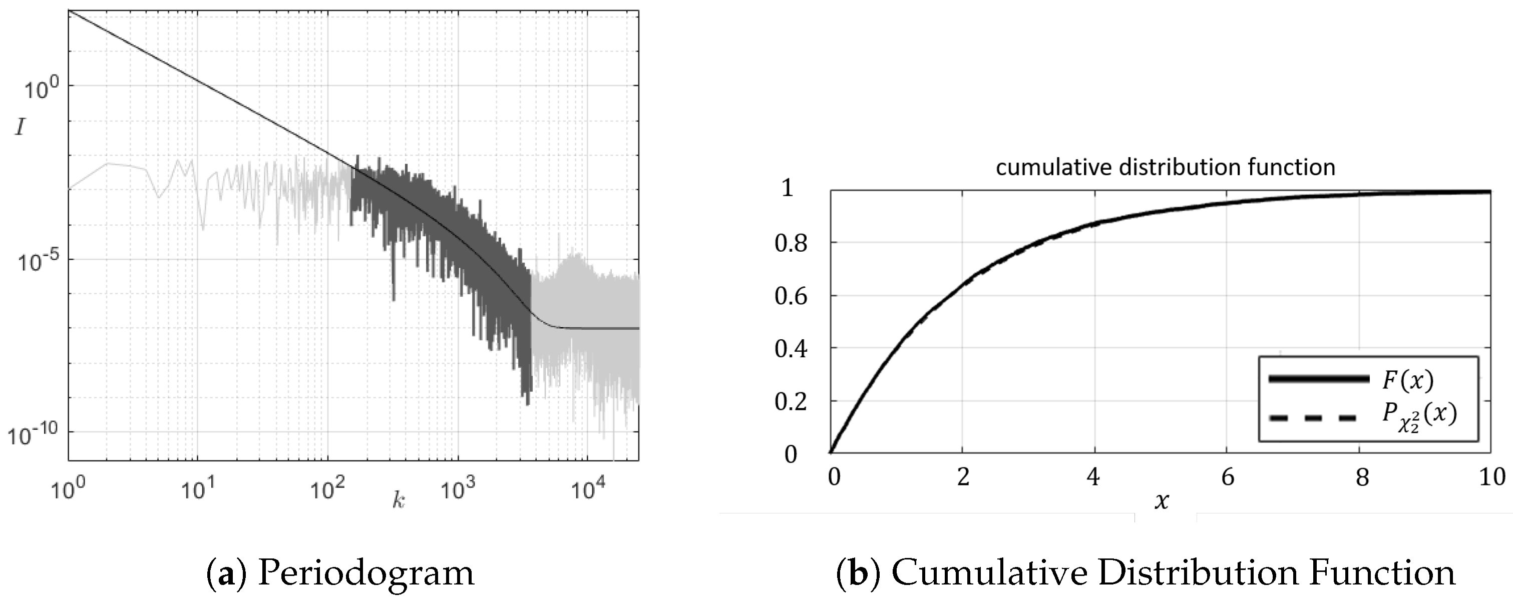
2.3.1. Spectrum Fitting Method

The data analysis methodology is explained in detail in [28], as well as in [25,25]. For the convenience of the reader, herein we provide a brief overview of the spectrum fitting method.
The analyzed data constitutes a time-series of measurements from the anemometer. To analyze the spectral properties of the fluctuations, we constructed a Fast Fourier transform (FFT) of the fluctuations. Assuming the real and imaginary components of the FFT represent a pair of identical, independent, normally distributed random values, the residuals should be chi-square distributed. MLE was employed to the fit parameters for a given fitting window [47]. To verify the statistical validity of the fit, a goodness-of-fit score p A D was computed [25,36,48,49,50]. The confidence intervals were computed by a Monte-Carlo method from a previous work [28].
The process allows for rapid computation of the fit parameters yielding the lowest uncertainties and their associated goodness-of-fit score.

2.3.2. Effect of the Fitting Interval

We approximated the data with a compound function S ( k ) k α exp ( β k ) . The exponential component of this function exp ( β k ) is scale-dependent, and defines a natural length scale | β | 1 . The power-law component k α is scale-invariant, and a substantial span of k values is required for confident parameter fitting and accurate fit evaluation. In the realistic experimental data considered in our work, the range of k values is relatively short, and the choice of the fit interval may influence the compound function parameters α and β . In order to identify the best fitting interval, to ensure the accuracy of our results and to preempt misinterpretations, we scrupulously investigated the dependence of the compound function parameters α and β on the the left cut-off k l and the right cut-off k r of the interval k [ k l , k r ] over which the fit was performed [25,28]. Such effects are known to exist in realistic turbulent processes [14,16,17,32].

3. Data Analysis Results

In this section, we employed the spectrum fitting method to scrupulously analyze the RT mixing data for fluctuations of the three velocity components in the experiments [12]. We investigated the properties of the fluctuations of the specific kinetic energy for the stream-wise u 2 and cross-tank w 2 velocity components, and we outlined those for the cross-stream velocity component v 2 studied in detail earlier [28]. We aimed to understand and answer the following questions: Can RT mixing exhibit dynamic anisotropy at very late times?; Can RT mixing be similar to isotropic and homogeneous canonical turbulence?; What are the properties of RT mixing in the environment of the experiments [12]? These three questions motivated and framed our study.

3.1. Stream-Wise Velocity

3.1.1. Spectral Properties of the Data

We first analyzed fluctuations of the kinetic energy of the stream-wise velocity component u 2 in the direction of the co-flowing streams of the heavy and the light fluids. In this case, in the interval k 110 , 3700 , an MLE for compound spectra S ( k ) exp ( α ln ( k ) + β k ) provided fit parameters α = 1.06 ± 0.06 ,   β = ( 2.14 ± 0.05 ) × 10 3 . These results are illustrated by Figure 2. The fitted periodogram found excellent agreement in k 110 , 3700 (shaded in magenta), whereas, on the right, a noise level of S n o i s e = 10 7 accurately captured the large wave-number ( k > 3000 ) data.
For the stream-wise velocity component u 2 fluctuations spectra, Figure 3 presents the dependence of the parameters α and β of the compound function S ( k ) k α exp ( β k ) on the left and right cut-offs k l ( r ) , and on the fitting window, k [ k l , k r ] . The Figure illustrates how α and β varied for all the data (Figure 3a), and for the data in the fitting window with the strictest values of relative errors and with high goodness-of-fit (Figure 3b).
Figure 4 further illustrates the measures of the uncertainty in the estimations of the compound function parameters and the goodness-of-fit, including the dependence of the relative errors σ α / α (Figure 4a) and σ β / β (Figure 4c) and the Anderson–Darling test score p A D (Figure 4b) on the left and the right cut-offs k l ( r ) for all the data considered.

3.1.2. Analysis of Residuals and Goodness of Fit

Applying the Anderson–Darling test between the empirical Cumulative Distribution Function (CDF) of the observed residuals Y k and a χ 2 2 distribution yielded a goodness of fit value of p A D = 0.5073 0.05 , suggesting that the observed residuals were χ 2 2 distributed, and, thus, the fit was statistically valid. The uncertainties in the fit parameters were small with σ α / α = 5.52 % and σ β / β = 2.43 % , and the spectral fit was well-contained by the data. The certainty in the fit was further justified in the near-perfect overlap between the empirical CDF of the residuals Y k and the χ 2 2 distribution. This result is illustrated in Figure 2b.

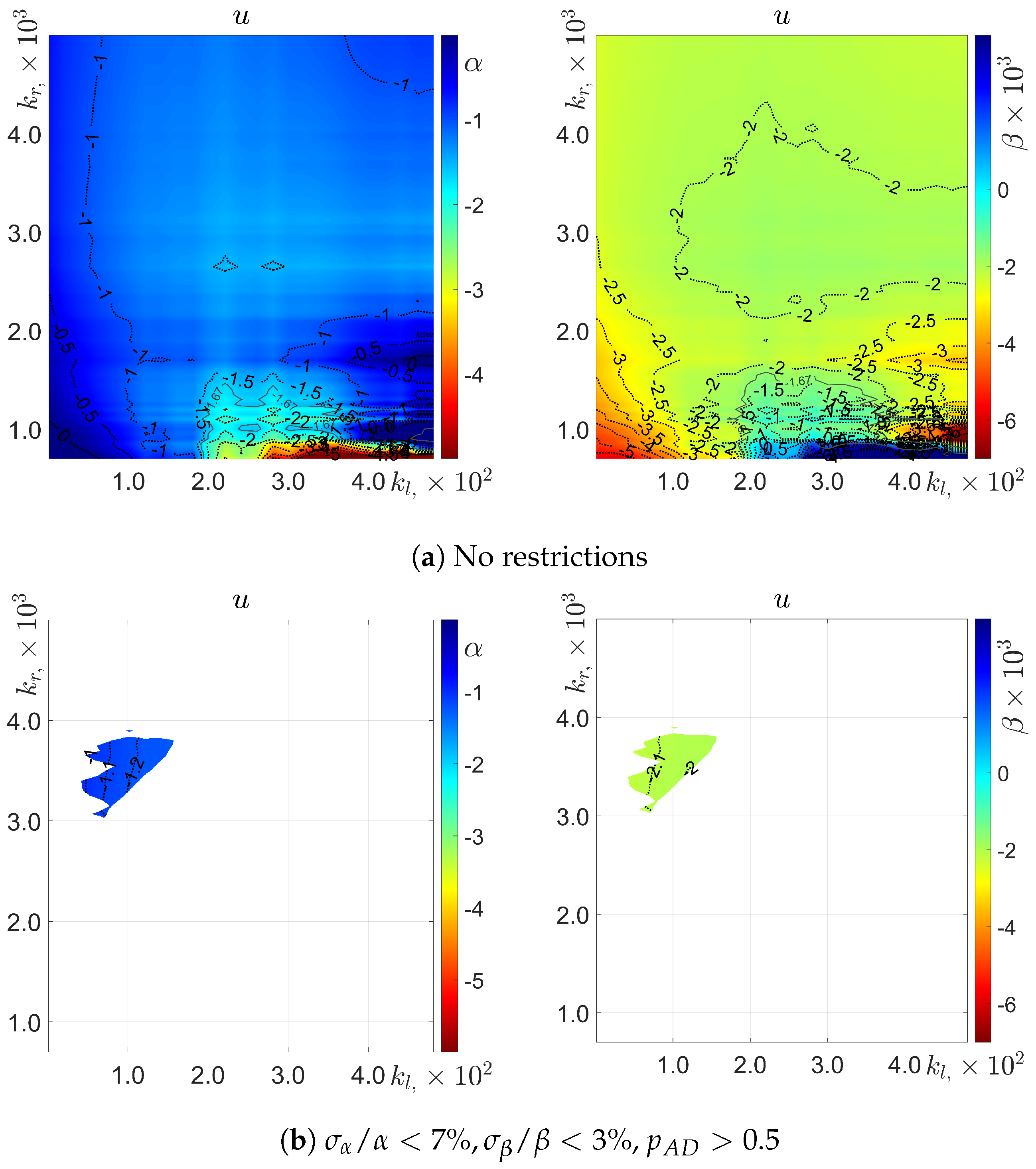
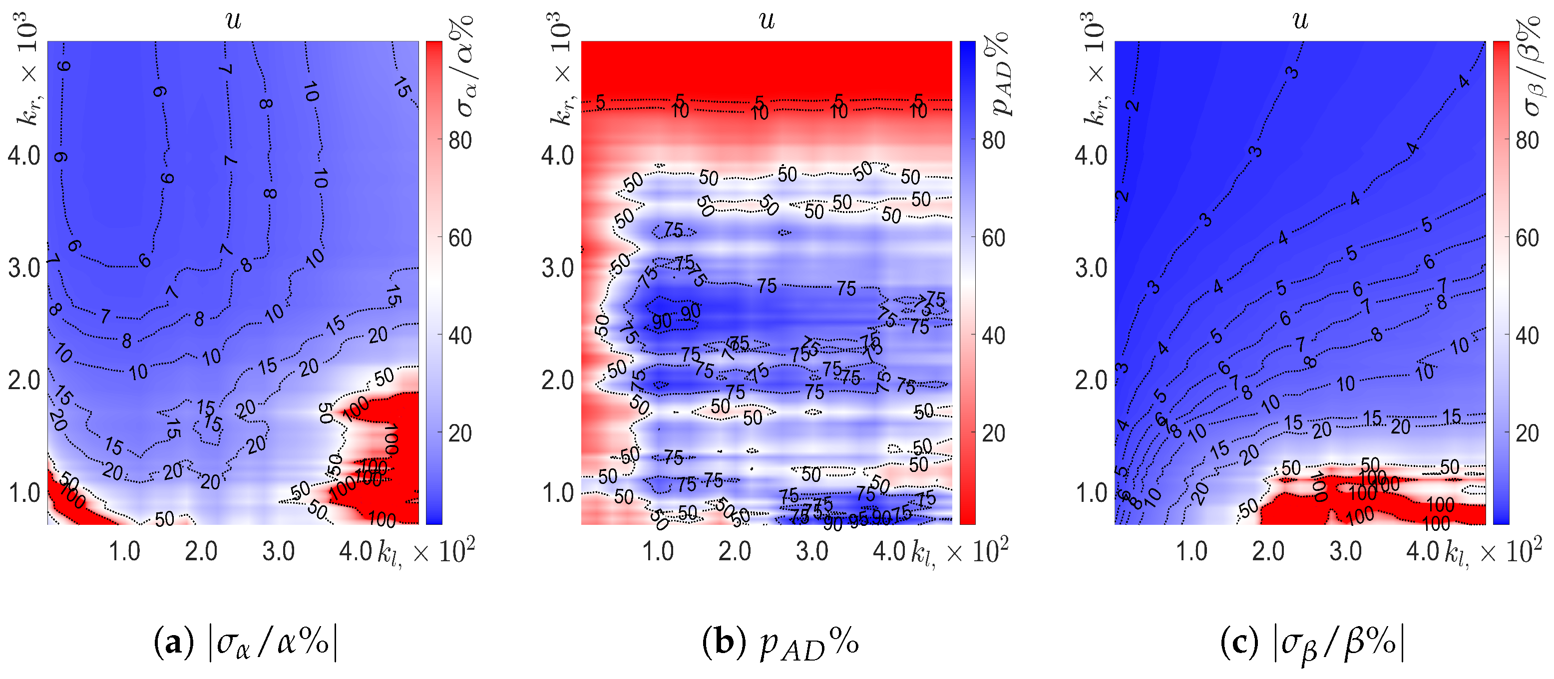
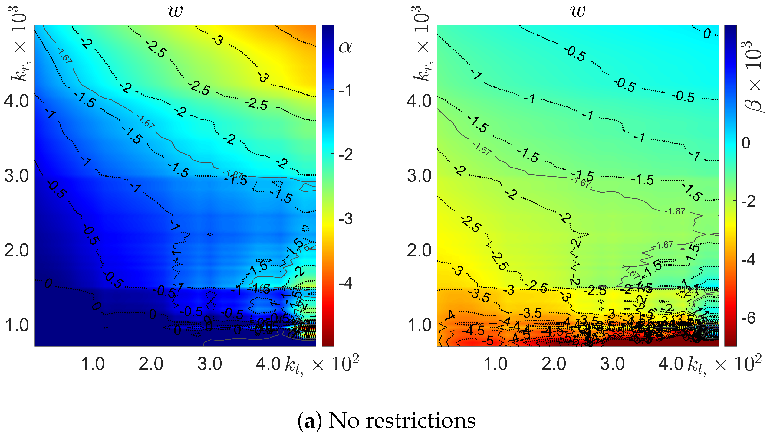
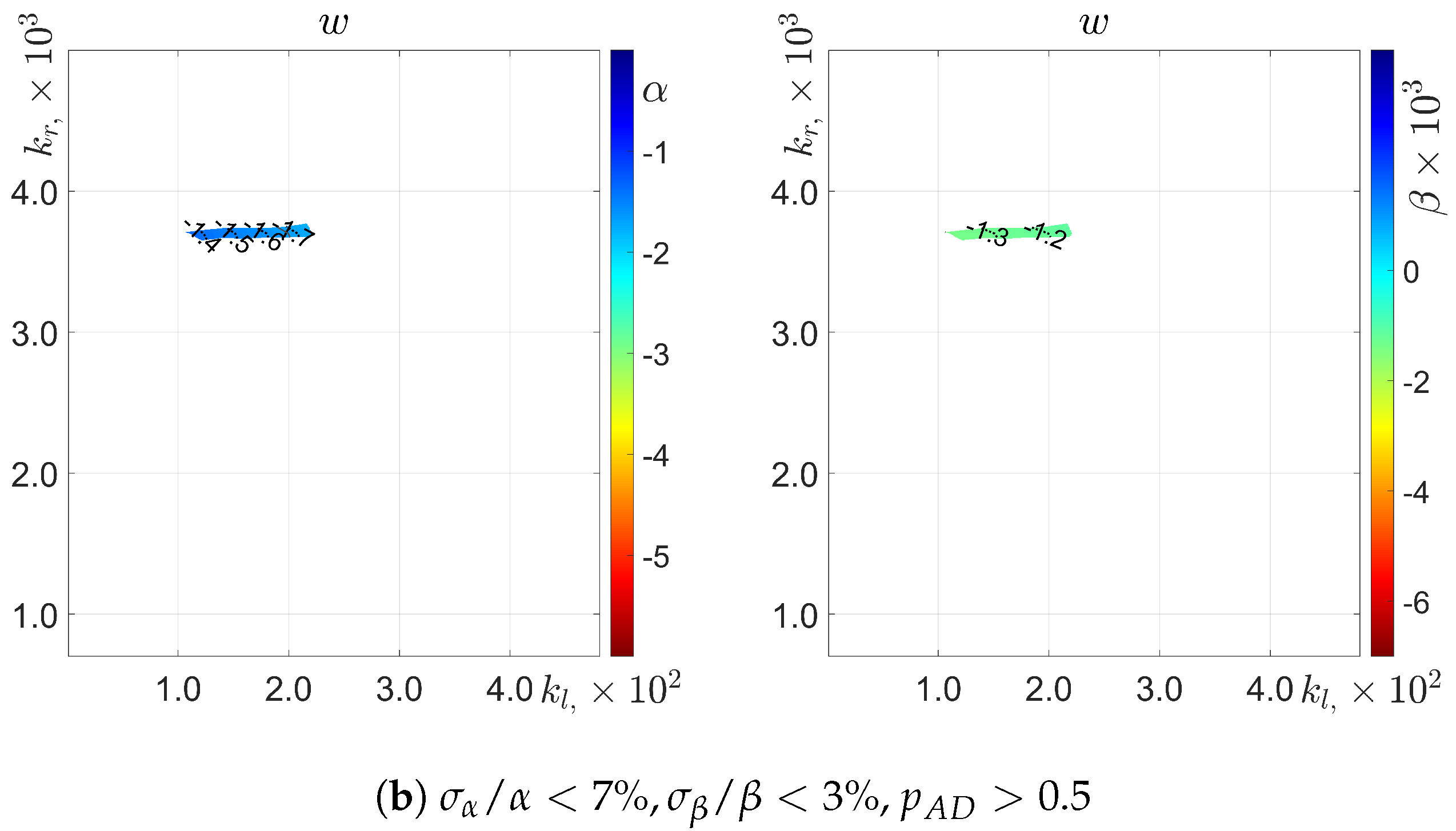
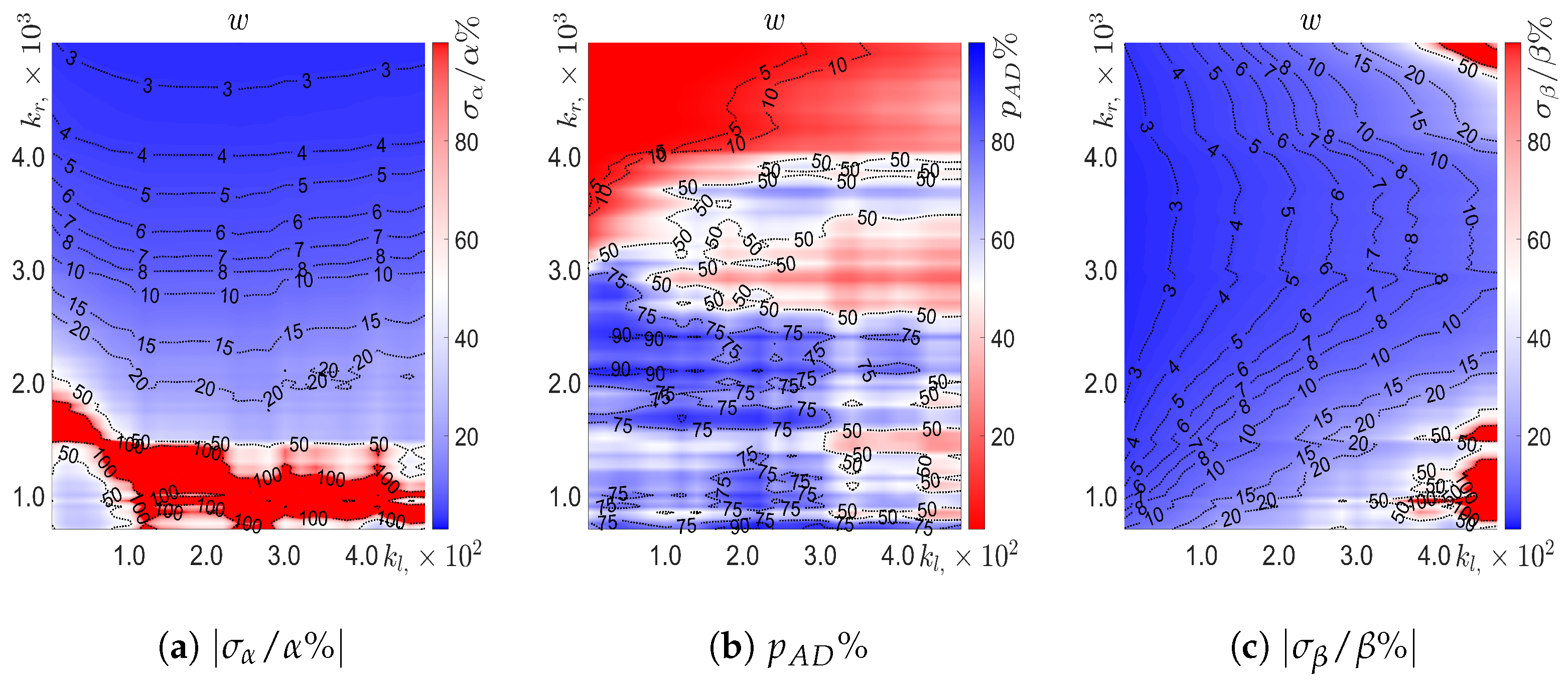
3.1.3. Effect of the Left and Right Cut-Off

The α values for the stream-wise velocity estimations ranged from α = 0.5 to α = 2.5 over the majority of the fit window, with very small outlier regions, in which α > 0.5 and α < 5 . For the vast majority of the fitting window, 1.5 < α < 1 , with divergences for the left cut-off, k l < 100 (for which α > 1 ), right cut-off, k r < 200 (with α varying from as high as α > 0 to as low as α < 5 ) and very large fit windows k l > 400 ,   k r > 4500 (with α > 1 ).
The estimations of β were somewhat more varied, ranging from β > 2 × 10 3 down to β < 5 × 10 3 . The estimated values were relatively stable for right cut-offs k r > 2000 , with the estimated β values being 2.5 × 10 3 < β < 2 × 10 3 in this region, except for a central window region with k l > 100 and 2500 < k r < 3500 ), in which 2 × 10 3 < β 1.75 × 10 3 . For right cut-offs below the region with k r < 2000 estimates, the values of β varied wildly, being highly affected by the variations over the source and integral parts of the spectrum, and with estimations ranging from β < 6 × 10 3 up to β > 4 × 10 3 .
The uncertainty in estimating α was inverse to the width of the fit window, with the lowest uncertainty σ α / α < 6 % being achieved for 20 < k l < 150 and k r > 3000 . The uncertainty was relatively symmetric about k l = 80 , with the uncertainty increasing as the left cut-off deviated from k l = 80 and as the right cut-off k r decreased. There were two small regions for which the estimation for α should be discounted: the corner defined by k r < 1000 ,   k l < 200 and the corner defined by k r < 2000 ,   k l > 350 .
The uncertainty of β was similarly inverse to the fit window, with the minimum uncertainty σ β / β < 2 % being achieved in the region k l < 20 ,   k r > 3500 . The dependence on the left cut-off k l was stronger than on the right cut-off k r for k r < 2000 and for k l < 200 . There was a small region, k l > 200 ,   k r < 1250 , for which constructing a fit was impossible, with uncertainties starting at σ β / β > 50 % and ranging to σ β / β 100 % .
Overall, the goodness of fit value in the estimating the fit parameters was above the threshold for rejection. The resultant range is presented in Figure 3b.

3.2. Cross-Tank Velocities

3.2.1. Spectral Properties of the Data

We now consider the fluctuations spectra of the kinetic energy of the cross-tank velocity component w 2 in the direction normal to the acceleration and to the direction of the co-flowing streams. In this case, for a broad interval k 150 , 3700 , the MLE fit of the data with a compound function S ( k ) exp ( α ln ( k ) + β k ) with α = 1.49 ± 0.07 and β = ( 1.30 ± 0.05 ) × 10 3 and with p A D = 0.6382 0.05 , which implied excellent goodness of fit and confidence in the fit parameters. The estimated noise S n o i s e 10 7 captured the behavior of the right of the periodogram ( k > 4000 ). These results are illustrated in Figure 5.
For the cross-tank velocity w 2 fluctuations spectra, Figure 6 presents the dependence of the parameters α and β of the compound function S ( k ) k α exp ( β k ) on the left and right cut-offs k l ( r ) and on the fitting window, k [ k l , k r ] . The Figure illustrates how α and β varied for all the data (Figure 6a); and for the data in the fitting window with the strictest values of relative errors and with high goodness-of-fit (Figure 6b).
Figure 7 further illustrates the measures of the uncertainty in the estimations of the compound function parameters and the goodness-of-fit, including the dependence of the relative errors σ α / α (Figure 7a) and σ β / β (Figure 7c) and the Anderson–Darling test score p A D (Figure 7b) on the left and the right cut-offs k l ( r ) for all the data considered.

3.2.2. Analysis of Residuals and Goodness of Fit

We applied the resultant fitted function to determine the observed residuals Y k , and tested the null hypothesis that the residuals were χ 2 2 distributed. Testing the hypothesis between the empirical CDF of the residuals and the CDF of the χ 2 2 distribution yielded a goodness of fit value of p A D = 0.5382 0.05 . Hence, the null hypothesis could not be rejected. This confidence in the fit was corroborated by the tight visual agreement between the empirical Cumulative Distribution Function (CDF) of the residuals and the CDF of the χ 2 2 distribution. This is illustrated by Figure 5b. In addition, the fitted function precisely captured the behavior of the periodogram and the uncertainty in the fit parameters was small, with σ α / α = 2.96 % and σ β / β = 3.98 % . This is illustrated by Figure 5a. The resultant fitted function was, thus, an accurate prescription of RT mixing dynamics.

3.2.3. Effect of the Left and Right Cut-Offs

The distribution of estimated α values varied from α < 3 to α > 0 . The estimation of α decreased as the right cut-off k r increased, and increased as the left cut-off k l increased, with the dependence on the left cut-off k l being more significant than the dependence on the right cut-off k r for k l < 350 ,   k r > 1500 and for k r > 4000 . For the small region k r < 1500 and for k r > 4000 . For the small region k r < 1500 ,   k l > 450 , the estimations for α varied greatly, due to the high sensitivity of the dynamics to the integral and inertial ranges. For small left and right cut-offs k l < 400 ,   k r < 1200 , corresponding to only the integral and inertial ranges, the estimation provided α 0 , over which range the velocity fluctuations appeared almost entirely scale-independent.
The distribution of estimated β values ranged from β 0 to β < 6 × 10 3 , but only varied from β 0 to β 3 × 10 3 for k r > 1500 . For k l > 200 (and k r > 1500 ), the dependence on the left cut-off was significantly greater than on the right cut-off. In a similar manner to the estimations for α , the fit yielded greatly fluctuating parameter estimations in the region k r < 1500 ,   k l > 450 , even more so than in the rest of the k r < 1500 range. In the regions wherein α was estimated as α 0 , the MLE yielded β 3 × 10 3 , in agreement with existing literature.
The uncertainty in the estimation of α was nearly independent of the left cut-off k l , except in the regions k l < 100 ( k l > 40 ), wherein the uncertainty in α decreased (increased) with increasing k l . The uncertainty in α generally decreased with increasing k r , in correspondence with the larger contribution of the near-dissipation and dissipative regimes. For k r < 1500 , k l > 100 and for 1500 < k r < 2000 and k l < 100 , the uncertainty in estimating α was σ α / α 100 % , and was excluded from consideration.
The uncertainty in estimating β had a more complex dependence on the left and right cut-offs than the uncertainty in α . For the fixed left cut-off, k l , the uncertainty in estimating β was minimized in the region 3000 < k r < 3500 . For the right cut-offs k r greater than (less than) the bounds of this region, the uncertainty was increasing (decreasing) in k r . For the fixed right cut-off k r , the uncertainty in estimating β was increasing for increasing left cut-off. Overall, the uncertainty gave the appearance of a minimum uncertainty at k l = 0 ,   k r = 3250 , outward from which the uncertainty increased with distance from this point, with a stronger dependence on the left cut-off k l than the right cutoff k r . There existed regions, with k l > 400 and k r > 4750 , and with k l > 400 and k r > 1500 m in which the fit became untenable, with uncertainties of σ β / β 100 % .
The goodness of fit score, as evaluated by the Anderson–Darling test, was much less regular than for the other parameters and varied a great deal in nearly all regions. For the region bounded by the line segment between k l = 0 ,   k r = 3500 and k l = 280 ,   k r = 5000 , the goodness of fit value was p A D < 0.05 < 0.10 and necessarily rejected. For k l > 100 ,   k r > 3600 and k l < 100 ,   k r > 3000 , the goodness of fit p A D < 0.5 . There was a large region of p A D < 0.5 for k l > 170 ,   1600 < k r < 3400 and several small patches of uncertain fits ( p A D < 0.5 ) in the domain k l > 300 ,   k r < 2000 . For the rest of the domain, the goodness of fit varied from 0.5 < p A D < 0.95 , with various, seemingly uncorrelated, regions with p A D > 0.75 ; commenting on these is, statistically, meaningless.

3.3. Cross-Stream Velocity

The properties of fluctuations of the kinetic energy v 2 of the cross-stream velocity component v in the direction of the acceleration g were scrupulously analyzed in our earlier work [28]. We briefly outline the obtained results. In this case, for the compound function S ( k ) k α exp ( β k ) , the MLE yielded the fit parameters α = 2.04 ± 0.06 and β = ( 1.02 ± 0.05 ) × 10 3 in the fitting interval k 100 , 4000 . The fit had a goodness of fit score p A D = 0.5699 0.05 , confirming the validity of the fit. The presumed noise level S n o i s e = 10 7 excellently captured the behavior of the data for k > 4000 . The fit was in excellent agreement with the periodogram of the data for the wave numbers considered k 100 , 4000 .

4. RT Mixing Characteristics in the Experiments

In this section, we identify the physics features of RT mixing in the experiments [12], from the results of our scrupulous data analysis guided by the group theory approach.

4.1. Flow Characteristics

To obtain the quantitative characteristics of RT mixing, we summarize our data analysis results in Table 1. Table 1 presents the characteristic quantities for each of the fluctuation spectra diagnosed in the experiments; namely, these are the estimated values of the parameters α and β of the compound function S ( k ) k α exp ( β k ) , the left k l and the right k r cut-offs of the fitting interval k [ k l , k r ] , and the span of scales l g ( k r / k l ) , with l g = l o g 10 .
We further evaluated the characteristic scales set by the exponential decay factor 1 / | β | of the compound function S ( k ) k α exp ( β k ) . Table 2 presents the value 1 / | β | , the corresponding wave-vector k * = 1 / | β | H and the length scale l * = 2 π / k * of the fluctuations spectra of each of the velocity components.
We also provide, here, for the reader’s convenience, the characteristic scales in the setup A1S0 in the RT mixing experiments [12]. Table 3 presents the scales set by the acceleration g, including the values of the wave-vector k ν and the length scale l ν . It also provides the scales set by the deterministic noise U ^ , including the values of the wave-vector k ^ ν and the length scale l ^ ν . The deterministic noise was due to the inaccuracy of the magnitude of the velocity of the co-flowing streams, U ^ = 0.01 U , in the experiments [12].

4.2. Anomalous Scaling

According to our data analysis results, the fluctuations spectra in RT mixing in realistic fluids can be represented by a product of a power-law and an exponential, S ( k ) k α exp ( β k ) . In the compound function S ( k ) , the power-law k α captured the self-similar dynamics at relatively large scales, whereas the exponential exp ( β k ) described the scale-dependent dynamics at small scales. These results were consistent with our theoretical foundations, and with the classical works, Equations (1)–(4) [9,13,14,17,26].

4.3. Dynamic Anisotropy

The results of our data analysis unambiguously exposed the dynamic anisotropy of RT mixing in realistic environments, such as the experiments in [12], and were in good agreement with the group theory results. The dynamic anisotropy was revealed in the different values of the power-law exponents α and the exponential decay factors β in the spectral shapes S ( k ) of the kinetic energy fluctuations in distinct velocity components. See Table 1 and Table 2, Figure 2a and Figure 5a, Equations (1)–(4) and Ref. [28].
Our data analysis found the following properties of fluctuations spectra of the velocity components v 2 , u 2 , w 2 , see Table 1 and Table 2 and Ref. [28]. In these spectra, the self-similar spectral part k α was the steepest, α 2 , for the cross-stream velocity v 2 in the direction of the acceleration. Furthermore, it was the most gradual, α 1 , for the stream-wise velocity u 2 in the direction of the co-flowing streams. The scale-dependent spectral part exp ( β k ) had the smallest magnitude of the exponential decay factor, | β | = 1.02 × 10 3 , and the smallest associated length scale, l * 7.69 × 10 3 [m], for the cross-stream velocity v 2 . It had the largest magnitude of the exponential decay factor, | β | = 2.14 × 10 3 , and the largest associated length scale, l * 3.89 × 10 2 [m], for the stream-wise velocity u 2 . These results were consistent with our theoretical foundation Equations (1), (3) and (4), and highlighted a number of relevant physics properties of RT mixing [12].
The fluctuations of the cross-stream velocity v 2 in the direction of the acceleration were discussed in detail in our recent work [28]. They are defined by the acceleration g. This is illustrated by the exponent α of the power-law, with the experimental value α = 2.04 being within 2 % of the theoretical value α = 2 . This is also illustrated by the characteristic length scale l * = 7.69 × 10 3 [m], which was set by the exponential decay factor | β | = 1.02 , and which was close, within 30 % , to the length scale l ν set by the acceleration g, and by the kinematic viscosity ν . See Table 1, Table 2 and Table 3, Equation (1), Section 2.1.2.
The fluctuations of the stream-wise velocity u 2 in the direction of the co-flowing streams were set by the deterministic experimental conditions. This was revealed by the exponent α of the power-law, with the experimental value α = 1.06 being close, within 6 % , to the theoretical value α = 1 . This was also revealed by the characteristic scale of length l * = 1.61 × 10 2 [m], which was defined by the exponential decay factor | β | = 2.14 , and which was within 3 % of the length scale l ^ ν , determined by the deterministic noise; the velocity scale U ^ and the kinematic viscosity ν . See Table 1, Table 2 and Table 3, Equation (3).
Recalling that, in the RT mixing experimental setup A1S0, the reported accuracy of the velocity magnitudes of the co-flowing streams, U = U 1 = U 2 , was within 4 % ; the data analysis, thus, suggested that even the slightest shear caused by a small deterministic noise ( U ^ = 0.01 U ) was sensed by RT mixing flow at very late times. The strong sensitivity of RT mixing to the deterministic conditions was consistent with the theoretical foundations and was also observed in other experiments [12,24,39].
The fluctuations of the cross-tank velocity w 2 (which was in the direction normal to the acceleration and to the velocity of the co-flowing streams) were set by the combined effects of the acceleration and the deterministic conditions. This was evidenced by the exponent α of the power-law, with experimental value α = 1.49 being within 0.07 % of α = 3 / 2 , which was the mean of the theoretical values of α = 2 and α = 1 of the cross-stream and stream-wise velocities, respectively. This was further confirmed by the characteristic length scale l * = 9.80 × 10 3 [m] set by the exponential decay factor | β | = 1.30 , which was within 20 % of a length scale 1.18 × 10 2 [m], which was the mean of the length scales l * = 7.69 × 10 3 [m] and l * = 1.61 × 10 2 [m] for v 2 and u 2 , respectively. See Table 1, Table 2 and Table 3, Equation (4). Note also that the power-law exponent for the w 2 fluctuations α = 1.49 was the closest (within 12 % ) to the exponent 5 / 3 for the canonical Kolmogorov turbulence [34,35,42].

4.4. Dynamic Bias

Our data analysis unambiguously revealed the dynamic bias of RT mixing dynamics in realistic experimental environments; thus, achieving good agreement with the group theory results. See Table 1 and Table 2, Figure 2a and Figure 5a, Equations (1)–(4) and Ref. [28].
Particularly, our data analysis exposed the sensitivity of the late time RT dynamics to the deterministic (the initial and the flow) conditions. This property of RT mixing is explained by group theory foundations, which have also explained similar observations in other RT mixing experiments with Reynolds numbers up to 3.2 × 10 6 for a broad range of setups and conditions [9,11,24,39,41].
While for any initial conditions the RT flow is expected to evolve toward a mixing regime with self-similarly growing amplitude in the acceleration direction, the RT dynamics in the normal directions can be scale-dependent and influenced by the deterministic conditions. We call this sensitivity to deterministic conditions dynamic bias. In our data analysis, the dynamic bias of RT mixing is revealed in the values of the power-law exponent α and the exponential decay factor β of the specific kinetic energy of the stream-wise u 2 velocity component. It is also revealed in the span of scales of fluctuations of the velocities ( v 2 , u 2 , w 2 ) . See Table 1, Table 2 and Table 3, Figure 2, Figure 3 and Figure 4.
For the velocity component u 2 , the exponent was α = 1.06 and the exponential decay factor was | β | = 2.14 , with associated length-scale l * = 1.61 × 10 2 [m]. These experimental values were in good agreement with the theoretical values set by the velocity scale U ^ and the kinematic viscosity ν , with α = 1 and l ^ ν = 1.50 × 10 2 [m]. They evidenced that the stream-wise dynamics in the direction of the co-flowing streams was influenced by the deterministic noise caused by the 1 % uncertainty of the velocity magnitude of the co-flowing stream U ^ = 0.01 U , U = U 1 = U 2 . See Table 1 and Table 3, Equation (3).
The other indicator of the dynamic bias of RT mixing was the relatively short span of scales. The experimental values of l g ( k r / k l ) for the velocity components ( v 2 , u 2 , w 2 ) were ( 1.60 , 1.53 , 1.39 ) , respectively. This experimental span of scales was substantially, 3 -fold, shorter than the span of scales predicted for canonical turbulence. The latter depended on the Reynolds number as l g ( R e 3 / 4 ) and was estimated as l g ( R e 3 / 4 ) 4.53 for R e = 3.4 × 10 4 . The short span of scales diagnosed in the experiments revealed that, in RT mixing, the velocity fluctuations are deterministic rather than stochastic in nature [9,24,30,34,35].

4.5. Analysis Method and Data Interpretation

Since RT mixing is sensitive to deterministic bias and is statistically unsteady, some discussion is required on the effect of the data analysis method on data interpretations [9,10,14,24,25,26,27,29,45].
To obtain physics properties of RT mixing in realistic environments, we analyzed raw unprocessed data and we applied compound functions to describe the fluctuations spectra of the diagnosed quantities. In the compound function S ( k ) k α exp ( β k ) , the power-law k α captures the self-invariant part of the spectrum at relatively large length scales, k k ν , and the exponential exp ( β k ) captures the scale-dependent part of the spectrum at relatively small length scales, k k ν .
To precisely evaluate the exponent α (the exponential decay factor β ), one needs to grasp accurately, and with ample statistics, the dynamics at relatively small (large) length scales, with k k ν ( k k ν ). An appropriate choice of the fitting interval k [ k l , k r ] , and its left (right) boundaries k l ( k r ) , is further required to enable a relatively broad span of scales l g ( k r / k l ) of the function S ( k ) , with small enough k l and with large enough k r . Hence, on the maps of α ( k l , k r ) and β ( k l , k r ) , accurate estimates of values α and β are expected to be located in the top left part in the plane ( k l , k r ) . This was fully consistent with our results. See Figure 3b and b and Ref. [28].
The goodness of fit is the most important aspect of the data analysis. Our previous work quantified goodness of fit by using the standard Kolmogorov–Smirnov (KS) test and the p K S score. Here, we employed the Anderson–Darling test and the parameter p A D , and we compared the residuals with the χ 2 2 distribution. We believe the Anderson–Darling test was more statistically suitable in our case, since the maximum likelihood estimator was computed from the same data set used to verify the fit without re-sampling. The goodness of fit analysis in our present work was consistent with that in the previous work; the dependence of the parameter p A D on the fitting window was qualitatively similar to that of the parameter p K S . See Figure 4b and Figure 7b, Ref. [28] and Refs. [25,36,48,49].
The dependence of the parameter p A D on the fitting interval in the plane ( k l , k r ) suggests that, in order for the residuals to be distributed according to the fitting technique assumptions, the statistical analysis should account for a significant number of modes on the left and on the right ends of the periodogram. Furthermore, in the regions k [ k l , k r ] , where the parameters α and β of the fitting function S ( k ) k α exp ( β k ) were precisely identified, the fit was excellent and the goodness-of-fit parameter value was high, p A D > 0.5 . A high precision and a high goodness of fit appear closely interrelated. We made a remarkable observation that, in statistically unsteady RT mixing, similarly to statistically steady processes, an old-school approach to quantify a value with small relative errors and with ample statistics works well. To our knowledge, such observations have not been discussed before. See Figure 2, Figure 3, Figure 4, Figure 5, Figure 6 and Figure 7 and Ref. [28].

4.6. Summary of Properties of RT Mixing

Our analysis of the data of fluctuations of each of the three velocity components identified important physics properties of RT mixing in realistic environments: the anomalous scaling, the dynamic anisotropy, and the dynamic bias. Specifically, the following were identified: (i) In RT mixing the fluctuations spectra differ substantially from the spectra of canonical Kolmogorov turbulence; (ii) In RT mixing, the fluctuations of the specific kinetic energy unambiguously exhibit dynamic anisotropy; (iii) RT mixing dynamics remain sensitive to deterministic conditions, even at very late times. These outcomes are consistent with group theory foundations and with other experiments. See Table 1 and Table 2, Figure 2, Figure 3, Figure 4, Figure 5, Figure 6 and Figure 7, Equations (1)–(4) [9,15,17,23,24,29,30,37,39,44,45,46,51].

4.7. Analysis Outcomes for Design of Experiments

We, herein, discuss the relevance of our data analysis to the design of experiments on RT mixing in fluids [10,12,19,24,39,41,52].
Traditionally, analysis of data is viewed as a tool for establishing fidelity of a theory by comparing theoretical predictions with experiments. The underlying assumptions are such that the theory is mathematically rigorous and physically accurate, whereas in the experiment, the conditions and parameters closely resemble theoretical assumptions, the diagnostics are accurate and non-intrusive, and the data have ample statistics [9,30,42].
The phenomena of Rayleigh–Taylor instability and RT mixing open new venues for data science, well beyond traditional considerations. Since RT dynamics is highly sensitive to deterministic (the initial and the flow) conditions, in addition to fidelity of the theory, one can employ the analysis of data for systematic control of experimental conditions, and for methodical improvement of experimental design [9,10,24].
For instance, the experiments [12,53] are designed to study the coupling of RT and KH dynamics and the late stages of RT mixing in a large domain. The pure RT dynamics is achieved in the setup A1S0, when the velocities of the co-flowing streams are the same, within a few percent, as U 1 = U 2 = U with | U ^ / U | 10 2 , where | U ^ | | U 1 U 2 | . The slight distinctions of the velocities of the co-flowing streams are assumed to have negligible effect on the late time RT mixing [12,53,54].
Our data analysis results unambiguously found that even that tiny a distinction may strongly influence the flow characteristics. Particularly, it may lead to significant, in several folds, departures in the parameters of the spectral shapes of the velocity components. This was illustrated by the values of α and β in the spectral shapes S ( k ) k α e β k for the fluctuations of the cross-stream and stream-wise velocity components, with α = 2.06 , β = 1.06 × 10 3 for v 2 and with α = 1.06 ,   β = 2.14 × 10 3 for u 2 ; see Table 1 and Figure 2 and Ref. [28]. The strong sensitivity of RT dynamics to the deterministic noise is consistent with the group theory results [9,26,29] and with experiments [24,41]. It also indicates a need in new approaches for experimental design [10].
Particularly, accurate probing and quantification of properties of RT mixing requires non-intrusive diagnostics of fast events, and ultra-high performance in space–time resolution, bandwidth, and data-acquisition rate, along with tight control of the initial and experimental conditions [10,17,24]. These requirements can be implemented in integrated experimental systems. The systems should integrate and incorporate state-of-the-art technology in motion control, precision mechanics, optical imaging, image processing, and digital signal processing, as well as data analysis methods [10,28]. For simultaneous measurements in space and in time of the interface dynamics and the flow fields, the experimental diagnostics may include, for example, particle image velocimetry, planar laser-induced fluorescence and holographic particle image velocimetry. By employing these diagnostic capabilities, one can accurately implement and diagnose RT mixing and can provide data suitable for a direct comparison with the group theory approach and numerical simulations [9,10,17,24,55,56,57].

4.8. Analysis Outcome for Numerical Simulations

Rayleigh–Taylor mixing is successfully modeled in numerical simulations employing various methods [55,56,58,59,60]. Traditionally, visual inspection is used to analyze smoothed post-processed numerical data, but our data analysis methodology can provide numerical simulations with a number of advantages, expanding the predictive modeling capabilities of simulations.
Our methodology can be applied to analyze both raw and processed numerical data. It can employ a broad class of fitting functions (e.g., a power-law, an exponential, a compound function) to study fluctuations spectra, structure functions, amplitude growth and growth rate, and other quantities. It can identify the fitting function parameters, including their mean values, relative errors and goodness-of-fit. It can investigate the dependence of the results on the fitting window and self-consistently identify the best fit interval. It can be used for both in-fly diagnostics and in-depth analysis of numerical data. We urge that high quality numerical simulations consider these advantages and incorporate our methodology [55,56,58,59,60].

4.9. Spectral Shapes in Turbulence and in RT Mixing

Compound functions of the form k α e β k are regularly employed in analysis of data from a broad range of realistic turbulent processes [13,14,15,16,17,32,33]. Success was found in the seminal works [13,14], which investigated the fluctuations spectra of isotropic, homogeneous turbulence at large, finite Reynolds numbers. With regards to physics, compound functions k α e β k describe processes in which self-similar k α and scale-dependent e β k dynamics interplay.
Rayleigh–Taylor mixing is anisotropic, inhomogeneous, non-local, and statistically unsteady, and is sensitive to deterministic conditions. Its properties depart from those of isotropic, homogeneous, local, statistically steady and stochastic Kolmogorov turbulence [9,24,40,41,44]. Rayleigh–Taylor mixing possesses a complex interplay of self-similar and scale-dependent dynamics. Hence, compound functions can be applied to analyze RT spectra, as in other physics processes.
The present work finds that, in addition to the shape k α e β k of fluctuations spectra, a thorough analysis of data is expected to include estimates of relative errors of fitting function parameters, evaluations of goodness of fit, and investigations of effects of fitting intervals on results. We urge numerical simulations and experiments of realistic turbulent processes and of Rayleigh–Taylor mixing to consider these findings and incorporate our methodology.

5. Discussion

We analyzed the fluctuations of three velocity components measured in a gas-flow RT experiment, by a hot-three-wire anemometer, using a group theory-guided data analysis method. The analysis elucidated some key features of the fluctuations spectra in realistic Rayleigh–Taylor instabilities.
We expounded the theoretical framework underpinning the aforementioned statistical method for diagnosing the physics and mathematical properties of RT mixing. The method employs a maximum likelihood estimate to estimate the best fit of the parameters and the standard errors associated with the fit parameters. To evaluate the goodness-of-fit, the Anderson–Darling test [25,36] is employed, including a new test statistic [28], (Section 4.1 and Section 4.2). By applying the method over all potential left and right cut-offs of the fitting interval, the effects of the fitting interval, left and right cut-offs, and the noise level on the model fit are investigated (Section 4.3). Group theory establishes the foundation for the method (Section 2.1.1, Section 2.1.2 and Section 2.1.3), justifying the functional form of the power density spectrum S ( k ) k α exp ( β k ) we have, herein, applied to analyze the time series (Section 2.1.4, Equation (5). Such forms have been applied in works on classical turbulence [13,14,26,29].
By optimizing each of the fit conditions, including the relative errors of the fit parameters, the goodness-of-fit, and the span of scales, we have identified the optimal fitting interval and determined the associated fit parameters (Section 5). We have further identified the resultant properties of RT mixing (Table 1 and Table 2, Figure 5, Figure 6 and Figure 7, Equations (1)–(4)).
The results of the data analysis indicate that RT mixing may depart substantially from canonical Kolmogorov turbulence, exhibiting dynamic isotropy, anomalous scaling properties, vastly different spectral properties, and the dependence of late-time dynamics on the deterministic conditions [9,11,13,14,15,16,17,24,26,27,32,34,35,37,39,41,44,51].
The data analysis method employed, herein, and the results of our investigation are applicable to future research in fluids, plasmas, and other materials which exhibit RT mixing, or other turbulence-adjacent phenomena. They may assist in informing new research at various scales [8,22].

6. Conclusions

This work investigated the properties of fluctuations in Rayleigh–Taylor mixing, based on analysis of experimental data. For fluctuations of the kinetic energy of each of three velocity components, we studied the fluctuations’ properties at large and at small scales. We found, with statistical confidence, that the spectral shapes of the fluctuations spectra in RT mixing experiments are at least as complex as compound functions, represented by a product of a power law and an exponential. The properties of the spectral shape parameters unambiguously identify the dynamic anisotropy and dynamic bias of Rayleigh–Taylor mixing in realistic environments, in agreement with group theory foundations, in conformity with experiments on high Reynolds number RT mixing and on accelerated turbulent flows, and in consistency with the anomalous properties of turbulent flows in realistic environments.

Author Contributions

Conceptualization, S.I.A.; Methodology, K.C.W. and S.I.A.; Software, K.C.W. and S.I.A.; Investigation, K.C.W. and S.I.A.; Data curation, K.C.W.; Writing—original draft, K.C.W. and S.I.A.; Supervision, S.I.A. All authors have read and agreed to the published version of the manuscript.

Funding

The authors appreciate the support of the National Science Foundation (USA) (Award No. 1404449), the Australian Research Council (AUS) (Award No. LE220100132), the Australian Government Research Training Program.

Institutional Review Board Statement

Not applicable.

Informed Consent Statement

Not applicable.

Data Availability Statement

The methods, the results and the data presented in this work are available to the readers in the paper.

Acknowledgments

The authors thank D. Ranjan for making the experimental data available for analysis, P. Suchandra for providing the information on the diagnostics and the resolution, and D. Pfefferle for permitting the use of the maximum likelihood estimator code. The authors deeply thank K.R. Sreenivasan for insightful comments and inspiring discussions.

Conflicts of Interest

The authors declare no conflict of interest.

References

  1. Herring, J.; Rilley, J.; Patterson, G.; Kraichnan, R. Growth of uncertainty in decaying isotropic turbulence. J. Atmos. Sci. 1973, 30, 997–1006. [Google Scholar] [CrossRef]
  2. Herring, J.; Orszag, S.; Kraichnan, R.; Fox, D. Decay of two-dimensional homogeneous turbulence. J. Fluid Mech. 1974, 66, 417–444. [Google Scholar] [CrossRef]
  3. Kraichnan, R.; Herring, J. A strain-based Lagrangian-history turbulence theory. J. Fluid Mech. 1978, 88, 355–367. [Google Scholar] [CrossRef]
  4. Gotoh, T.; Rogallo, J.; Herring, J.; Kraichnan, R. Lagrangian velocity correlations in homogeneous isotropic turbulence. Phys. Fluids A Fluid Dyn. 1993, 5, 2846–2864. [Google Scholar] [CrossRef]
  5. Chen, S.; Doolen, G.; Herring, J.; Kraichnan, R.; Orszag, S.; She, Z. Far-dissipation range of turbulence. Phys. Rev. Lett. 1993, 70, 3051–3054. [Google Scholar] [CrossRef] [PubMed] [Green Version]
  6. Kerr, R.; Herring, J. Prandtl number dependence of Nusselt number in direct numerical simulations. Phys. Scr. 2000, 419, 325–344. [Google Scholar] [CrossRef]
  7. Herring, J.; Kimura, Y. Some issues and problems of stably stratified turbulence. Phys. Scr. 2013, T155, 014031. [Google Scholar] [CrossRef]
  8. Abarzhi, S.; Gauthier, S.; Sreenivasan, K. Turbulent mixing and beyond: Non-equilibrium processes from atomistic to astrophysical scales I. Philos. Trans. R. Soc. A Math. Phys. Eng. Sci. 2013, 371, 20120436. [Google Scholar] [CrossRef] [PubMed]
  9. Abarzhi, S. Review of theoretical modelling approaches of Rayleigh-Taylor instabilities and turbulent mixing. Philos. Trans. R. Soc. A Math. Phys. Eng. Sci. 2010, 368, 1809–1828. [Google Scholar] [CrossRef] [PubMed]
  10. Orlov, S.; Abarzhi, S.; Oh, S.; Barbastathis, G.; Sreenivasan, K. High-performance holographic technologies for fluid-dynamics experiments. Philos. Trans. R. Soc. A Math. Phys. Eng. Sci. 2010, 368, 1705–1737. [Google Scholar] [CrossRef] [PubMed] [Green Version]
  11. Anisimov, S.; Drake, R.; Gauthier, S.; Meshkov, E.; Abarzhi, S. What is certain and what is not so certain in our knowledge of Rayleigh-Taylor mixing? Philos. Trans. R. Soc. A Math. Phys. Eng. Sci. 2013, 371, 20130266. [Google Scholar] [CrossRef] [PubMed]
  12. Akula, B.; Suchandra, P.; Mikhaeil, M.; Ranjan, D. Dynamics of unstably stratified free shear flows: An experimental investigation of coupled Kelvin–Helmholtz and Rayleigh–Taylor instability. J. Fluid Mech. 2017, 816, 619–660. [Google Scholar] [CrossRef]
  13. Kraichnan, R. The structure of isotropic turbulence at very high Reynolds numbers. J. Fluid Mech. 1959, 5, 497–543. [Google Scholar] [CrossRef] [Green Version]
  14. Sreenivasan, K. On the scaling of the turbulence energy dissipation rate. Phys. Fluids 1984, 27, 1048–1051. [Google Scholar] [CrossRef]
  15. Sreenivasan, K.; Antonia, R. The phenomenology of small-scale turbulence. Annu. Rev. Fluid Mech. 1997, 28, 435–472. [Google Scholar] [CrossRef] [Green Version]
  16. Pouquet, A.; Mininni, P. The interplay between helicity and rotation in turbulence: Implications for scaling laws and small-scale dynamics. Philos. Trans. R. Soc. A 2010, 368, 1635–1662. [Google Scholar] [CrossRef] [PubMed]
  17. Sreenivasan, K. Turbulent mixing: A perspective. Proc. Natl. Acad. Sci. USA 2019, 116, 18175–18183. [Google Scholar] [CrossRef] [Green Version]
  18. Strutt, R.J.L. Investigation of the Character of the Equilibrium of an Incompressible Heavy Fluid of Variable Density. Proc. Lond. Math. Soc. 1883, s1-14, 170–177. [Google Scholar] [CrossRef]
  19. Davies, R.; Taylor, G. The mechanics of large bubbles rising through extended liquids and through liquids in tubes. Proc. R. Soc. London. Ser. A Math. Phys. Sci. 1950, 200, 375–390. [Google Scholar] [CrossRef]
  20. Arnett, W.D. Supernovae and Nucleosynthesis: An Investigation of the History of Matter, from the Big Bang to the Present; Princeton Series in Astrophysics; Princeton University Press: Princeton, NJ, USA, 1996. [Google Scholar]
  21. Haan, S.W.; Lindl, J.D.; Callahan, D.A.; Clark, D.S.; Salmonson, J.D.; Hammel, B.A.; Atherton, L.J.; Cook, R.C.; Edwards, M.J.; Glenzer, S.; et al. Point design targets, specifications, and requirements for the 2010 ignition campaign on the National Ignition Facility. Phys. Plasmas 2011, 18, 051001. [Google Scholar] [CrossRef]
  22. Abarzhi, S.; Goddard, W. Interfaces and mixing: Nonequilibrium transport across the scales. Proc. Natl. Acad. Sci. USA 2019, 116, 18171–18174. [Google Scholar] [CrossRef] [PubMed] [Green Version]
  23. Remington, B.; Park, H.S.; Casey, D.; Cavallo, R.; Clark, D.; Huntington, C.; Kuranz, C.; Miles, A.; Nagel, S.; Raman, K.; et al. Rayleigh-Taylor instabilities in high-energy density settings on the National Ignition Facility. Proc. Natl. Acad. Sci. USA 2019, 116, 18223–18228. [Google Scholar] [CrossRef] [PubMed] [Green Version]
  24. Meshkov, E.; Abarzhi, S. Group theory and jelly’s experiment of Rayleigh–Taylor instability and Rayleigh–Taylor interfacial mixing. Fluid Dyn. Res. 2019, 51, 065502. [Google Scholar] [CrossRef] [Green Version]
  25. Pfefferlé, D.; Abarzhi, S. Whittle maximum likelihood estimate of spectral properties of Rayleigh-Taylor interfacial mixing using hot-wire anemometry experimental data. Phys. Rev. E 2020, 102, 053107, Erratum in 2022, 106, 019901. [Google Scholar] [CrossRef] [PubMed]
  26. Abarzhi, S. Self-similar interfacial mixing with variable acceleration. Phys. Fluids 2021, 33, 122110. [Google Scholar] [CrossRef]
  27. Abarzhi, S.; Sreenivasan, K. Self-similar Rayleigh-Taylor mixing with accelerations varying in time and in space. Proc. Natl. Acad. Sci. USA 2022, 119, e2118589119. [Google Scholar] [CrossRef]
  28. Williams, K.; Abarzhi, S. Fluctuations spectra of specific kinetic energy, density, and mass flux in Rayleigh–Taylor mixing. Phys. Fluids 2023, 34, 122188. [Google Scholar] [CrossRef]
  29. Abarzhi, S.I. On fundamentals of Rayleigh-Taylor turbulent mixing. EPL Europhysics Lett. 2010, 91, 35001. [Google Scholar] [CrossRef]
  30. Sreenivasan, K. Fluid turbulence. Rev. Mod. Phys. 1999, 71, S383–S395. [Google Scholar] [CrossRef]
  31. Bershadskii, A. Distributed chaos and turbulence in Bénard-Marangoni and Rayleigh-Bénard convection. arXiv 2019, arXiv:1903.05018. [Google Scholar]
  32. Klewicki, J.; Chini, G.; Gibson, J. Prospectus: Towards the development of high-fidelity models of wall turbulence at large Reynolds number. Philos. Trans. R. Soc. A 2017, 375, 20160092. [Google Scholar] [CrossRef] [Green Version]
  33. Yakhot, V.; Donzis, D. Emergence of multiscaling in a random-force stirred fluid. Phys. Rev. Lett. 2017, 119, 044501. [Google Scholar] [CrossRef] [Green Version]
  34. Kolmogorov, A. The Local Structure of Turbulence in Incompressible Viscous Fluid for Very Large Reynolds’ Numbers. Dokl. Akad. Nauk SSSR 1941, 30, 299–303. [Google Scholar]
  35. Kolmogorov, A. On the degeneracy of isotropic turbulence in an incompressible viscous fluid. Dokl. Akad. Nauk SSSR 1941, 31, 538–541. [Google Scholar]
  36. Anderson, T.; Darling, D. A Test of Goodness-of-Fit. J. Am. Stat. Assoc. 1954, 49, 765–769. [Google Scholar] [CrossRef]
  37. Robey, H.F.; Zhou, Y.; Buckingham, A.C.; Keiter, P.; Remington, B.; Drake, R. The time scale for the transition to turbulence in a high Reynolds number, accelerated flow. Phys. Plasmas 2003, 10, 614–622. [Google Scholar] [CrossRef] [Green Version]
  38. Dalziel, S.; Linden, P.; Youngs, D. Self-similarity and internal structure of turbulence induced by Rayleigh–Taylor instability. J. Fluid Mech. 1999, 399, 1–48. [Google Scholar] [CrossRef] [Green Version]
  39. Meshkov, E.E. Studies of Hydrodynamic Instabilities in Laboratory Experiments; FGUC-VNIIEF: Sarov, Russia, 2006; ISBN 5-9515-0069-9. (In Russian) [Google Scholar]
  40. Swisher, N.; Kuranz, C.; Arnett, W.; Hurricane, O.; Robey, H.; Remington, B.; Abarzhi, S. Rayleigh-Taylor mixing in supernova experiments. Phys. Plasmas 2015, 22, 102707. [Google Scholar] [CrossRef]
  41. Meshkov, E. Some peculiar features of hydrodynamic instability development. Philos. Trans. R. Soc. A Math. Phys. Eng. Sci. 2013, 371, 20120288. [Google Scholar] [CrossRef]
  42. Landau, L.; Lifshitz, E. Course of Theoretical Physics; Elsevier Science: Amsterdam, The Netherlands, 1987; Volume I–X. [Google Scholar]
  43. Abarzhi, S.; Gorobets, A.; Sreenivasan, K. Rayleigh–Taylor turbulent mixing of immiscible, miscible and stratified fluids. Phys. Fluids 2005, 17, 081705. [Google Scholar] [CrossRef] [Green Version]
  44. Abarzhi, S.; Bhowmick, A.; Naveh, A.; Pandian, A.; Swisher, N.; Stellingwerf, R.; Arnett, W. Supernova, nuclear synthesis, fluid instabilities, and interfacial mixing. Proc. Natl. Acad. Sci. USA 2019, 116, 18184–18192. [Google Scholar] [CrossRef] [PubMed] [Green Version]
  45. Abarzhi, S.; Hill, D.; Williams, K.; Wright, C. Buoyancy and drag in Rayleigh-Taylor and Richtmyer-Meshkov linear, nonlinear and mixing dynamics. Appl. Math. Lett. 2022, 31, 108036. [Google Scholar] [CrossRef]
  46. Abarzhi, S.; Hill, D.; Williams, K.; Li, J.; Remington, B.; Martinez, D.; Arnett, W. Fluid dynamics mathematical aspects of supernova remnants. Phys. Fluids 2023, 35, 034106. [Google Scholar] [CrossRef]
  47. Whittle, P. Curve and Periodogram Smoothing. J. R. Stat. Soc. 1957, 19, 38–63. [Google Scholar] [CrossRef]
  48. Kolmogorov, A.N. Sulla Determinazione Empirica di una Legge di Distribuzione. Giorn. Dell’Inst. Ital. Attuari. 1933, 4, 83–91. [Google Scholar]
  49. Smirnov, N. Table for Estimating the Goodness of Fit of Empirical Distributions. Ann. Math. Statist. 1948, 19, 279–281. [Google Scholar] [CrossRef]
  50. Stephens, M.A. EDF Statistics for Goodness of Fit and Some Comparisons. J. Am. Stat. Assoc. 1987, 69, 730–737. [Google Scholar] [CrossRef]
  51. Narasimha, R.; Sreenivasan, K. Relaminarization in highly accelerated turbulent boundary layers. J. Fluid Mech. 1973, 61, 417–447. [Google Scholar] [CrossRef]
  52. Read, K. Experimental investigation of turbulent mixing by Rayleigh–Taylor instability. Phys. D 1984, 12, 45–58. [Google Scholar] [CrossRef]
  53. Kraft, W.; Banerjee, A.; Andrews, M. On hot-wire diagnostics in Rayleigh–Taylor mixing layers. Exp. Fluids 2009, 47, 49–68. [Google Scholar] [CrossRef]
  54. Akula, B.; Ranjan, D. Dynamics of buoyancy-driven flows at moderately high Atwood numbers. J. Fluid Mech. 2016, 795, 313–355. [Google Scholar] [CrossRef]
  55. Reynolds number effects on Rayleigh–Taylor instability with possible implications for type Ia supernovae. Nat. Phys. 2006, 2, 562–568. [CrossRef]
  56. Schilling, O. Self-similar Reynolds-averaged mechanical–scalar turbulence models for Rayleigh–Taylor, Richtmyer–Meshkov, and Kelvin–Helmholtz instability-induced mixing in the small Atwood number limit. Phys. Fluids 2021, 33, 085129. [Google Scholar] [CrossRef]
  57. Schumacher, J.; Sreenivasan, K. Colloquium: Unusual dynamics of convection in the Sun. Rev. Mod. Phys. 2022, 92, 041001. [Google Scholar] [CrossRef]
  58. Ristorcelli, J.; Clark, T. Rayleigh–Taylor turbulence: Self-similar analysis and direct numerical simulations. J. Fluid Mech. 2004, 507, 213–253. [Google Scholar] [CrossRef]
  59. Glimm, J.; Sharp, D.; Kaman, T.; Lim, H. New directions for Rayleigh-Taylor mixing. Philos. Trans. R. Soc. A Math. Phys. Eng. Sci. 2013, 371, 20120183. [Google Scholar] [CrossRef] [PubMed] [Green Version]
  60. Grinstein, F.; Saenz, J.; Germano, M. Coarse grained simulations of shock-driven turbulent material mixing. Phys. Fluids 2021, 33, 035131. [Google Scholar] [CrossRef]
Figure 1. Configuration of the experimental tank. The gas inflow is stream-wise (in the x-direction), with the gravity driving the flow against the cross-stream direction (y-direction) and with both the inflow and gravity being incident to the cross-tank (z) direction.
Atmosphere 14 01178 g001
Figure 2. (a) The estimated fluctuation spectra S ( k ) (black line) found tight agreement with the periodogram of the streamwise ( u 2 ) velocity fluctuation spectra in the region considered (magenta). (b) The Cumulative Distribution Function of the residuals closely followed that of the χ 2 2 distribution.
Atmosphere 14 01178 g002
Figure 3. Variations in the estimation of α (left) and β (right) as a function of the fit window for the stream-wise velocity u 2 fluctuations.
Atmosphere 14 01178 g003
Figure 4. Measures of uncertainty in obtaining α (a), the uncertainty in the estimation of β (c) and the goodness of fit score p A D (b) for stream-wise velocity u 2 fluctuations.
Atmosphere 14 01178 g004
Figure 5. (a) The estimated fluctuation spectra S ( k ) (black line) found tight agreement with the periodogram of the cross-tank velocity ( w 2 ) fluctuation spectra in the region considered (gray). (b) The Cumulative Distribution Function of the residuals closely followed that of the χ 2 2 distribution.
Atmosphere 14 01178 g005
Figure 6. Variations in the estimation of α (left) and β (right) as a function of the fit window for the cross-tank velocity w 2 fluctuations.
Atmosphere 14 01178 g006aAtmosphere 14 01178 g006b
Figure 7. Measures of uncertainty in obtaining α (a), the uncertainty in the estimation of β (c) and the goodness of fit score p A D (b) for the cross-tank velocity w 2 fluctuations.
Atmosphere 14 01178 g007
Table 1. Characteristics of the fluctuation spectra for each of the velocity components, including the parameters α and β of the compound function S ( k ) k α exp ( β k ) , the left k l and the right boundaries k r of the fitting interval, and the span of scales l g ( k r / k l ) .
Quantity α β k l H k r H lg ( k r / k l )
u 2 1.06 ± 0.06 ( 2.14 ± 0.05 ) × 10 3 1103700 1.53
w 2 1.49 ± 0.07 ( 1.30 ± 0.05 ) × 10 3 1503700 1.39
v 2 2.04 ± 0.06 ( 1.02 ± 0.05 ) × 10 3 1004000 1.60
Table 2. Characteristic scales set by the exponential decay factor β , including the value 1 / | β | , the corresponding wave-vector k * = 1 / | β | H and the length scale l * = 2 π / k * in the fluctuations spectra for each of the velocity components.
Quantity 1 / | β | k * , [ m 1 ] l * , [ m ]
u 2 4.67 × 10 2 3.89 × 10 2 1.61 × 10 2
w 2 7.69 × 10 2 6.41 × 10 2 9.80 × 10 3
v 2 9.80 × 10 2 8.17 × 10 2 7.69 × 10 3
Table 3. Characteristic scales in RT mixing experiments in the setup A1S0 set by the acceleration g ( k ν and l ν ) and by the deterministic noise U ^ ( k ^ ν and l ^ ν ).
k ν , [ m 1 ] l ν , [ m ] k ^ ν , [ m 1 ] l ^ ν , [ m ]
1.11 × 10 3 5.71 × 10 3 3.93 × 10 2 1.50 × 10 2
Disclaimer/Publisher’s Note: The statements, opinions and data contained in all publications are solely those of the individual author(s) and contributor(s) and not of MDPI and/or the editor(s). MDPI and/or the editor(s) disclaim responsibility for any injury to people or property resulting from any ideas, methods, instructions or products referred to in the content.

