

Downscaling Daily Satellite-Based Precipitation Estimates Using MODIS Cloud Optical and Microphysical Properties in Machine-Learning Models
 ,
,  ,
,
Abstract
:1. Introduction
2. Data
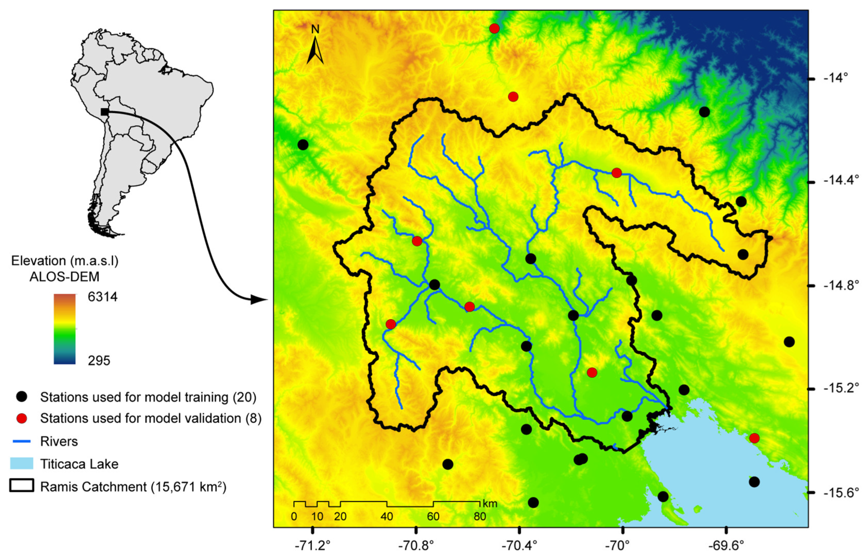
2.1. Study Area
2.2. Rain Gauges
2.3. Satellite-Based Precipitation Estimates: IMERG
2.4. Satellite Cloud Cover Properties: MODIS
2.5. Satellite-Based Temperature Estimates: CHIRTS
2.6. Digital Elevation Model: ALOS-DEM
3. Methods
3.1. Machine Learning Model: Random Forest
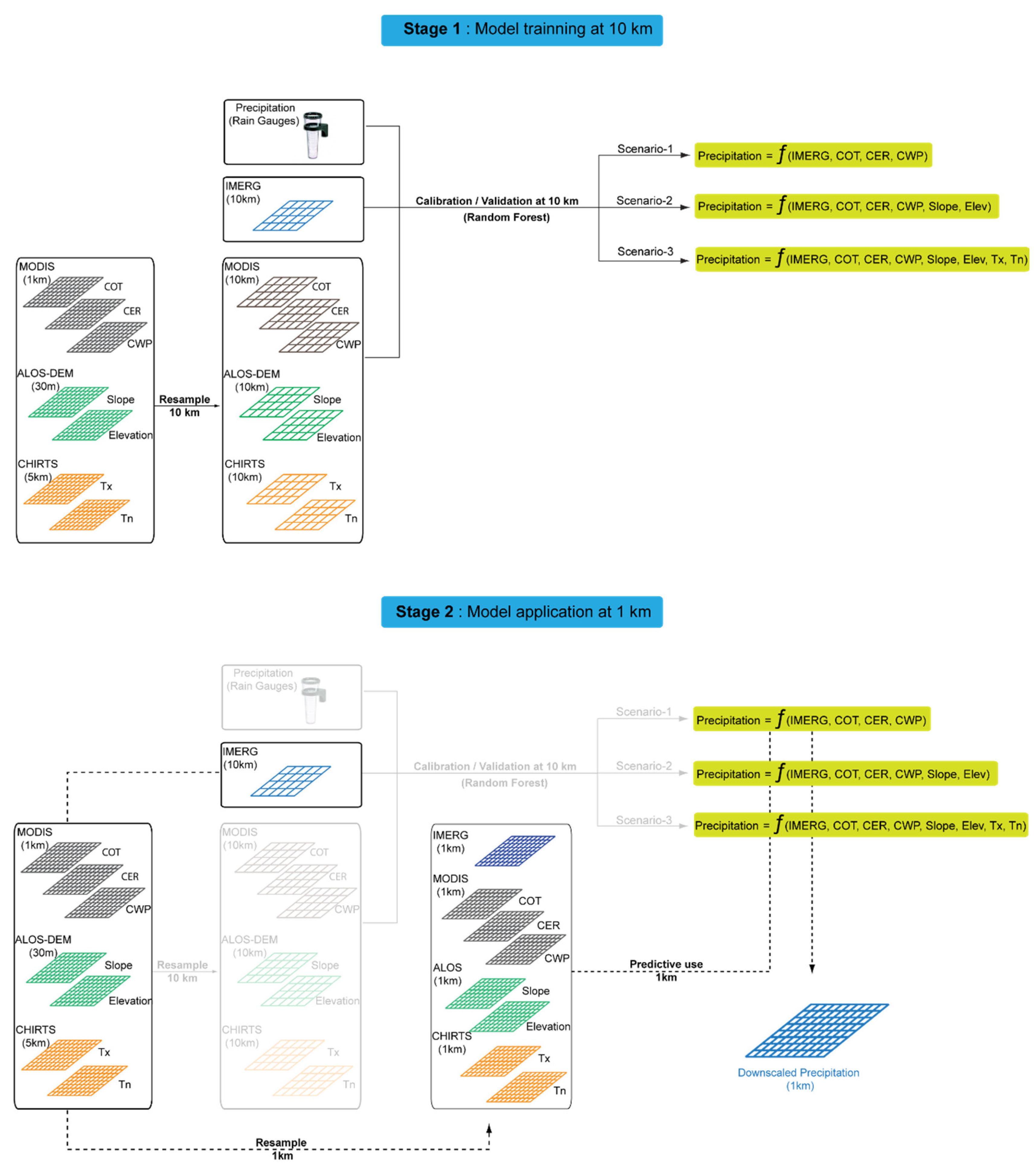
3.2. Downscaling Setup
3.3. Performance Evaluation Analysis
3.3.1. Quantitative Metrics
3.3.2. Categorical Metrics
4. Results and Discussion
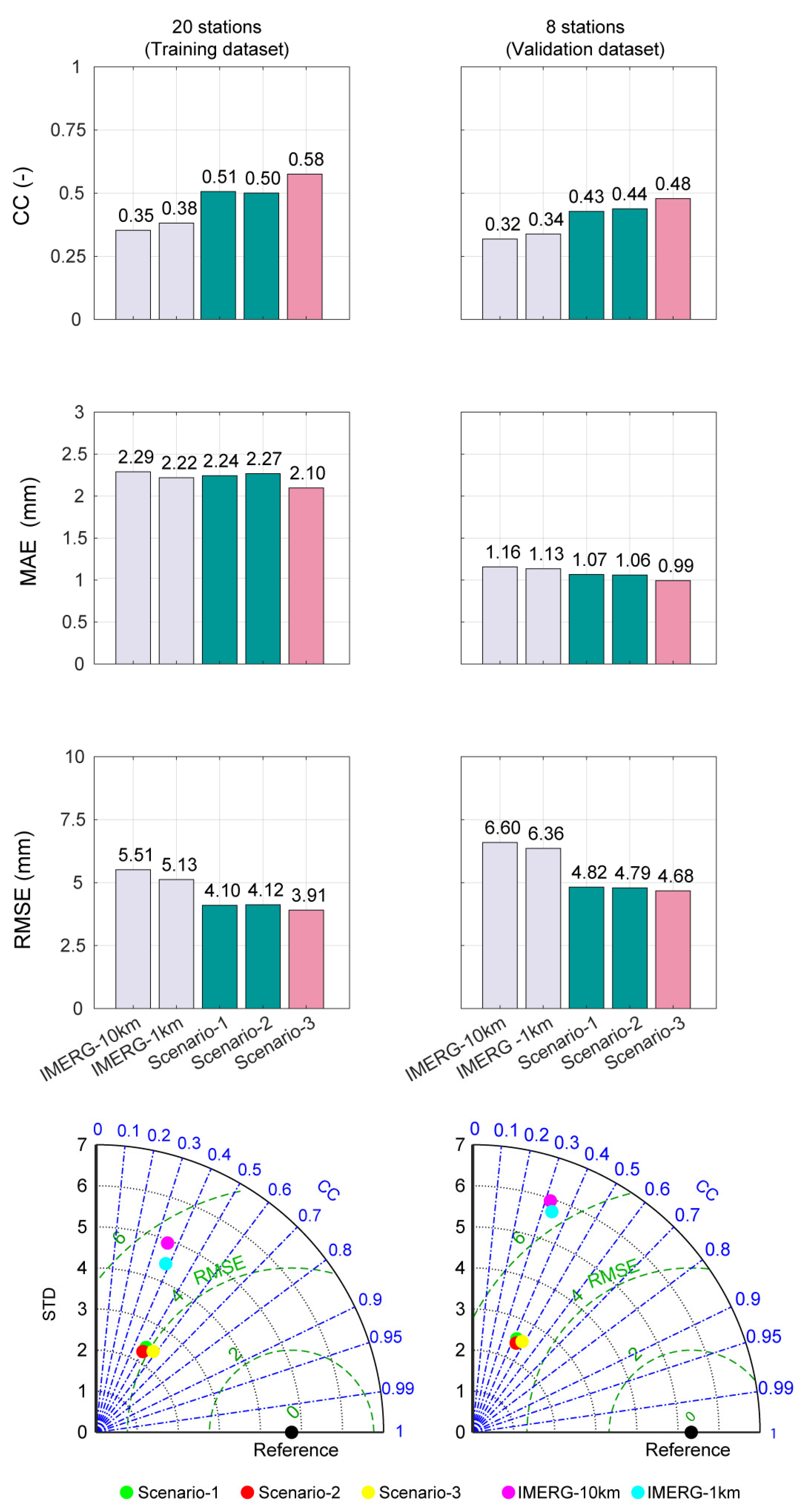
4.1. Evaluation of Results from Quantitative Indices
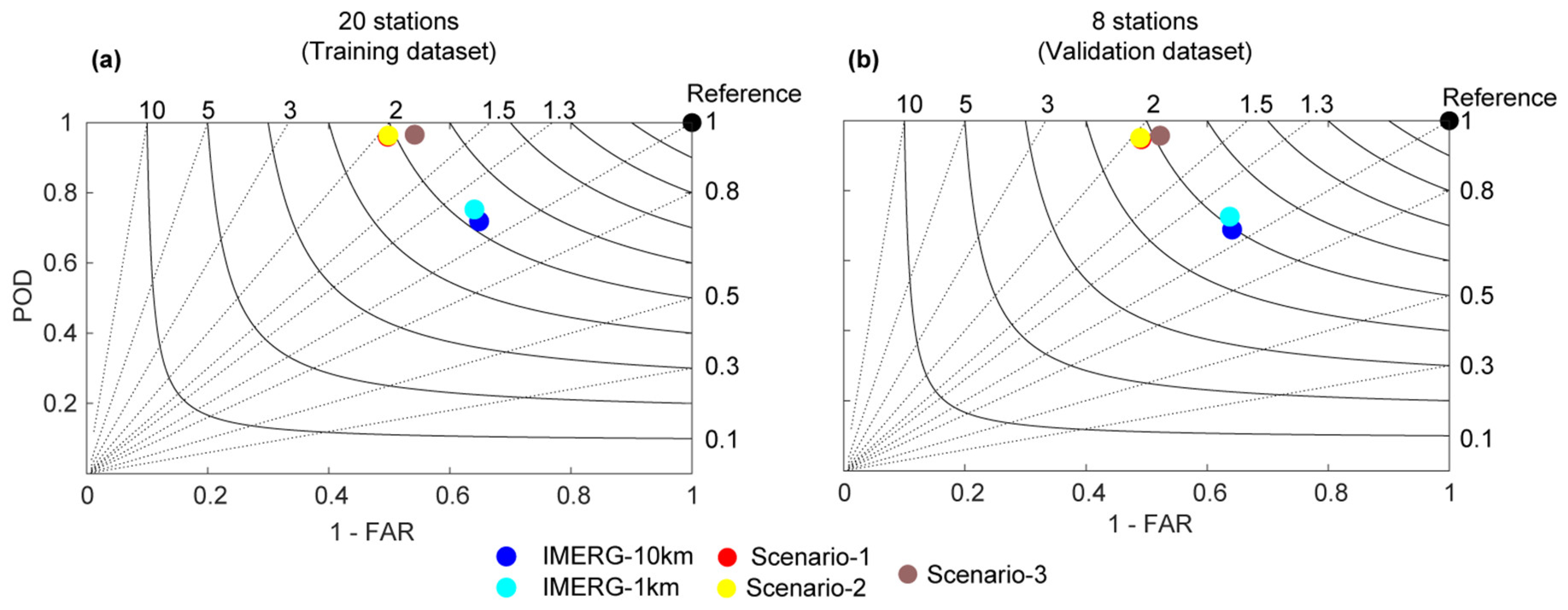
4.2. Evaluation from Qualitative Indices
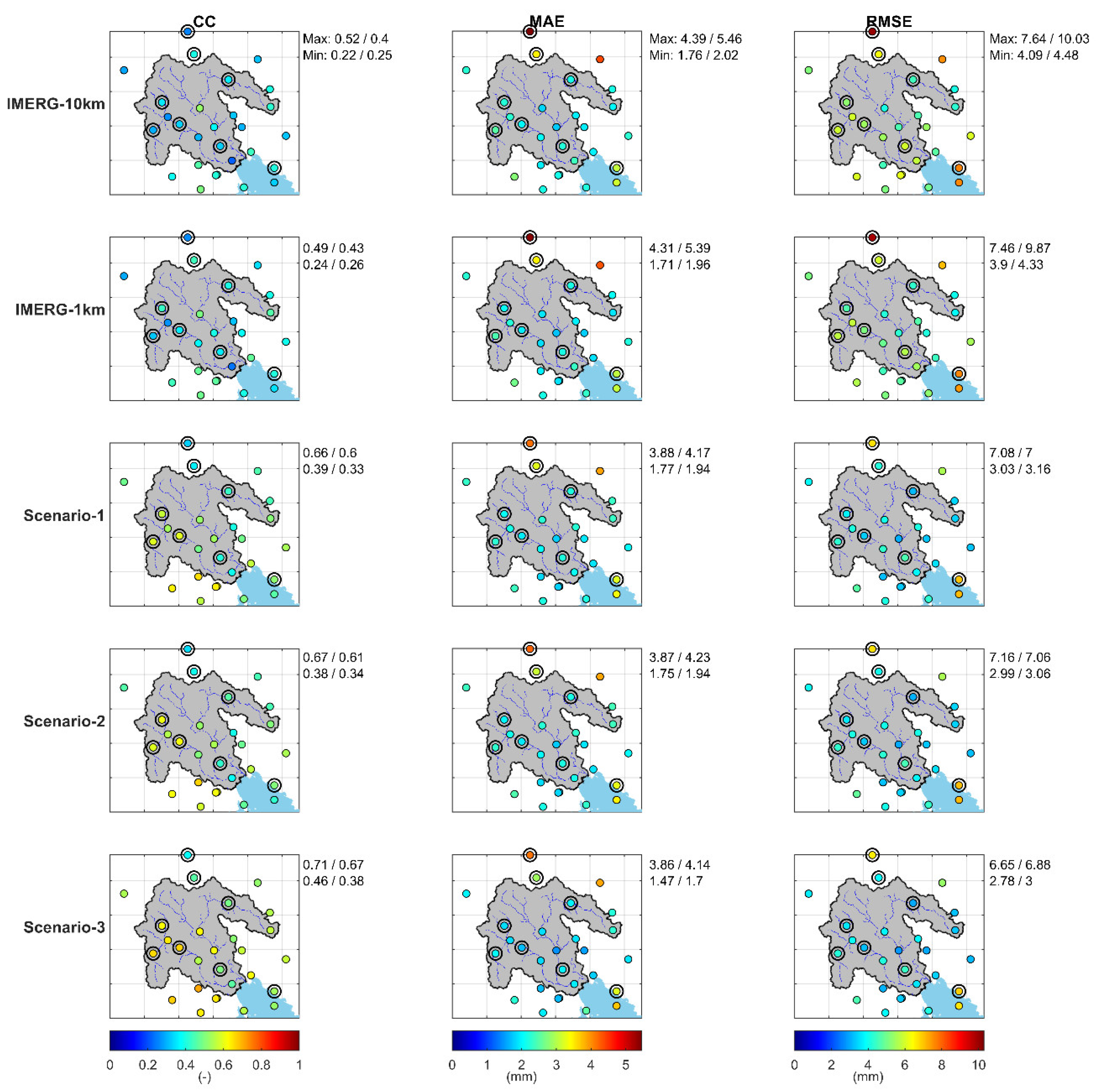
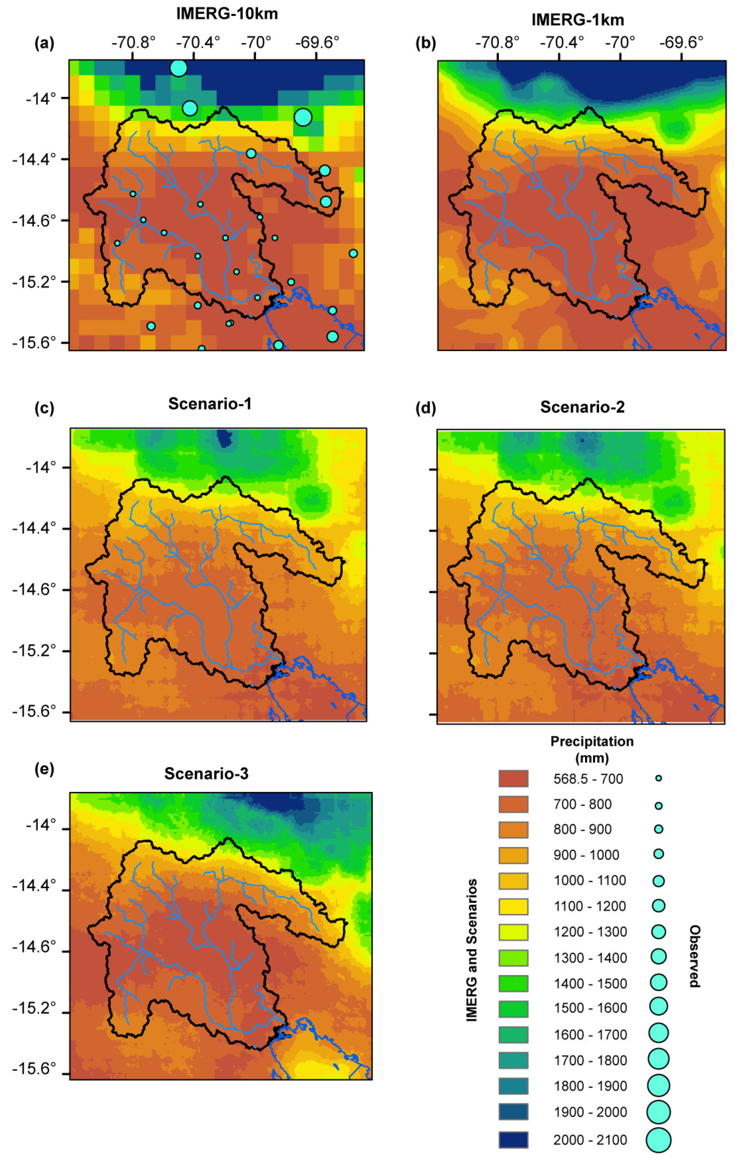
4.3. Assessment of the Precipitation Spatial Pattern
5. Conclusions
Author Contributions
Funding
Institutional Review Board Statement
Informed Consent Statement
Data Availability Statement
Conflicts of Interest
References
- Fallah, A.; Sungmin, O.; Orth, R. Climate-dependent propagation of precipitation uncertainty into the water cycle. Hydrol. Earth Syst. Sci. 2020, 24, 3725–3735. [Google Scholar] [CrossRef]
- Wild, M. The global energy balance as represented in CMIP6 climate models. Clim. Dyn. 2020, 55, 553–577. [Google Scholar] [CrossRef] [PubMed]
- Yang, D.; Yang, Y.; Xia, J. Hydrological cycle and water resources in a changing world: A review. Geogr. Sustain. 2021, 2, 115–122. [Google Scholar] [CrossRef]
- Allan, R.P.; Barlow, M.; Byrne, M.P.; Cherchi, A.; Douville, H.; Fowler, H.J.; Gan, T.Y.; Pendergrass, A.G.; Rosenfeld, D.; Swann, A.L.S.; et al. Advances in understanding large-scale responses of the water cycle to climate change. Ann. N. Y. Acad. Sci. 2020, 1472, 49–75. [Google Scholar] [CrossRef]
- Chen, F.; Gao, Y.; Wang, Y.; Li, X. A downscaling-merging method for high-resolution daily precipitation estimation. J. Hydrol. 2020, 581, 124414. [Google Scholar] [CrossRef]
- Satgé, F.; Bonnet, M.-P.; Gosset, M.; Molina, J.; Lima, W.H.Y.; Pillco Zolá, R.; Timouk, F.; Garnier, J. Assessment of satellite rainfall products over the Andean plateau. Atmos. Res. 2016, 167, 1–14. [Google Scholar] [CrossRef]
- Baez-Villanueva, O.M.; Zambrano-Bigiarini, M.; Ribbe, L.; Nauditt, A.; Giraldo-Osorio, J.D.; Thinh, N.X. Temporal and spatial evaluation of satellite rainfall estimates over different regions in Latin-America. Atmos. Res. 2018, 213, 34–50. [Google Scholar] [CrossRef]
- Sharifi, E.; Saghafian, B.; Steinacker, R. Downscaling Satellite Precipitation Estimates with Multiple Linear Regression, Artificial Neural Networks, and Spline Interpolation Techniques. J. Geophys. Res. Atmos. 2019, 124, 789–805. [Google Scholar] [CrossRef]
- Lei, H.; Zhao, H.; Ao, T. A two-step merging strategy for incorporating multi-source precipitation products and gauge observations using machine learning classification and regression over China. Hydrol. Earth Syst. Sci. 2022, 26, 2969–2995. [Google Scholar] [CrossRef]
- Liang, S.; Wang, J. (Eds.) Advanced Remote Sensing: Terrestrial Information Extraction and Applications, 2nd ed.; Academic Press: Amsterdam, The Netherlands, 2020; ISBN 978-0-12-815826-5. [Google Scholar]
- Goshime, D.W.; Absi, R.; Ledésert, B. Evaluation and Bias Correction of CHIRP Rainfall Estimate for Rainfall-Runoff Simulation over Lake Ziway Watershed, Ethiopia. Hydrology 2019, 6, 68. [Google Scholar] [CrossRef]
- Salimi, A.H.; Masoompour Samakosh, J.; Sharifi, E.; Hassanvand, M.R.; Noori, A.; von Rautenkranz, H. Optimized Artificial Neural Networks-Based Methods for Statistical Downscaling of Gridded Precipitation Data. Water 2019, 11, 1653. [Google Scholar] [CrossRef]
- Satgé, F.; Hussain, Y.; Molina-Carpio, J.; Pillco, R.; Laugner, C.; Akhter, G.; Bonnet, M. Reliability of SM2RAIN precipitation datasets in comparison to gauge observations and hydrological modelling over arid regions. Int. J. Climatol. 2021, 41, E517–E536. [Google Scholar] [CrossRef]
- Chiang, Y.-M.; Hsu, K.-L.; Chang, F.-J.; Hong, Y.; Sorooshian, S. Merging multiple precipitation sources for flash flood forecasting. J. Hydrol. 2007, 340, 183–196. [Google Scholar] [CrossRef]
- de Coning, E. Optimizing Satellite-Based Precipitation Estimation for Nowcasting of Rainfall and Flash Flood Events over the South African Domain. Remote Sens. 2013, 5, 5702–5724. [Google Scholar] [CrossRef]
- Saber, M.; Yilmaz, K. Evaluation and Bias Correction of Satellite-Based Rainfall Estimates for Modelling Flash Floods over the Mediterranean region: Application to Karpuz River Basin, Turkey. Water 2018, 10, 657. [Google Scholar] [CrossRef]
- Jiang, D.; Wang, K. The Role of Satellite-Based Remote Sensing in Improving Simulated Streamflow: A Review. Water 2019, 11, 1615. [Google Scholar] [CrossRef]
- Wang, Q.; Xia, J.; She, D.; Zhang, X.; Liu, J.; Zhang, Y. Assessment of four latest long-term satellite-based precipitation products in capturing the extreme precipitation and streamflow across a humid region of southern China. Atmos. Res. 2021, 257, 105554. [Google Scholar] [CrossRef]
- Satgé, F.; Xavier, A.; Pillco Zolá, R.; Hussain, Y.; Timouk, F.; Garnier, J.; Bonnet, M.-P. Comparative Assessments of the Latest GPM Mission’s Spatially Enhanced Satellite Rainfall Products over the Main Bolivian Watersheds. Remote Sens. 2017, 9, 369. [Google Scholar] [CrossRef]
- Zubieta, R.; Molina-Carpio, J.; Laqui, W.; Sulca, J.; Ilbay, M. Comparative Analysis of Climate Change Impacts on Meteorological, Hydrological, and Agricultural Droughts in the Lake Titicaca Basin. Water 2021, 13, 175. [Google Scholar] [CrossRef]
- Behrangi, A.; Hsu, K.; Imam, B.; Sorooshian, S.; Huffman, G.J.; Kuligowski, R.J. PERSIANN-MSA: A Precipitation Estimation Method from Satellite-Based Multispectral Analysis. J. Hydrometeorol. 2009, 10, 1414–1429. [Google Scholar] [CrossRef]
- Wang, J.; Petersen, W.A.; Wolff, D.B. Validation of Satellite-Based Precipitation Products from TRMM to GPM. Remote Sens. 2021, 13, 1745. [Google Scholar] [CrossRef]
- Wang, Z.; Zhong, R.; Lai, C.; Chen, J. Evaluation of the GPM IMERG satellite-based precipitation products and the hydrological utility. Atmos. Res. 2017, 196, 151–163. [Google Scholar] [CrossRef]
- Sun, L.; Lan, Y. Statistical downscaling of daily temperature and precipitation over China using deep learning neural models: Localization and comparison with other methods. Int. J. Climatol. 2021, 41, 1128–1147. [Google Scholar] [CrossRef]
- Wang, F.; Tian, D.; Lowe, L.; Kalin, L.; Lehrter, J. Deep Learning for Daily Precipitation and Temperature Downscaling. Water Resour. Res. 2021, 57, e2020WR029308. [Google Scholar] [CrossRef]
- Yan, X.; Chen, H.; Tian, B.; Sheng, S.; Wang, J.; Kim, J.-S. A Downscaling–Merging Scheme for Improving Daily Spatial Precipitation Estimates Based on Random Forest and Cokriging. Remote Sens. 2021, 13, 2040. [Google Scholar] [CrossRef]
- Pham, H.X.; Shamseldin, A.Y.; Melville, B.W. Projection of future extreme precipitation: A robust assessment of downscaled daily precipitation. Nat. Hazards 2021, 107, 311–329. [Google Scholar] [CrossRef]
- Xiang, L.; Xiang, J.; Guan, J.; Zhang, F.; Zhao, Y.; Zhang, L. A Novel Reference-Based and Gradient-Guided Deep Learning Model for Daily Precipitation Downscaling. Atmosphere 2022, 13, 511. [Google Scholar] [CrossRef]
- Ulloa, J.; Ballari, D.; Campozano, L.; Samaniego, E. Two-Step Downscaling of Trmm 3b43 V7 Precipitation in Contrasting Climatic Regions with Sparse Monitoring: The Case of Ecuador in Tropical South America. Remote Sens. 2017, 9, 758. [Google Scholar] [CrossRef]
- Xu, S.; Wu, C.; Wang, L.; Gonsamo, A.; Shen, Y.; Niu, Z. A new satellite-based monthly precipitation downscaling algorithm with non-stationary relationship between precipitation and land surface characteristics. Remote Sens. Environ. 2015, 162, 119–140. [Google Scholar] [CrossRef]
- Chen, C.; Hu, B.; Li, Y. Easy-to-use spatial random-forest-based downscaling-calibration method for producing precipitation data with high resolution and high accuracy. Hydrol. Earth Syst. Sci. 2021, 25, 5667–5682. [Google Scholar] [CrossRef]
- Karbalaye Ghorbanpour, A.; Hessels, T.; Moghim, S.; Afshar, A. Comparison and assessment of spatial downscaling methods for enhancing the accuracy of satellite-based precipitation over Lake Urmia Basin. J. Hydrol. 2021, 596, 126055. [Google Scholar] [CrossRef]
- Kobayashi, T.; Masuda, K. Effects of precipitation on the relationships between cloud optical thickness and drop size derived from space-borne measurements. Geophys. Res. Lett. 2008, 35, L24809. [Google Scholar] [CrossRef]
- Campos Braga, R.; Rosenfeld, D.; Krüger, O.O.; Ervens, B.; Holanda, B.A.; Wendisch, M.; Krisna, T.; Pöschl, U.; Andreae, M.O.; Voigt, C.; et al. Linear relationship between effective radius and precipitation water content near the top of convective clouds. Atmos. Chem. Phys. 2021, 21, 14079–14088. [Google Scholar] [CrossRef]
- Kobayashi, T.; Masuda, K. Changes in Cloud Optical Thickness and Cloud Drop Size Associated with Precipitation Measured with TRMM Satellite. J. Meteorol. Soc. Jpn. Ser. II 2009, 87, 593–600. [Google Scholar] [CrossRef]
- Gammons, C.H.; Slotton, D.G.; Gerbrandt, B.; Weight, W.; Young, C.A.; McNearny, R.L.; Cámac, E.; Calderón, R.; Tapia, H. Mercury concentrations of fish, river water, and sediment in the Río Ramis-Lake Titicaca watershed, Peru. Sci. Total Environ. 2006, 368, 637–648. [Google Scholar] [CrossRef]
- Satgé, F.; Ruelland, D.; Bonnet, M.-P.; Molina, J.; Pillco, R. Consistency of satellite-based precipitation products in space and over time compared with gauge observations and snow- hydrological modelling in the Lake Titicaca region. Hydrol. Earth Syst. Sci. 2019, 23, 595–619. [Google Scholar] [CrossRef]
- Lujano, E.; Sosa, J.D.; Lujano, R.; Lujano, A. Performance evaluation of hydrological models GR4J, HBV and SOCONT for the forecast of average daily flows in the Ramis river basin, Peru. Rev. Ing. UC 2020, 27, 189–199. [Google Scholar]
- Pillco Zolá, R.; Bengtsson, L.; Berndtsson, R.; Martí-Cardona, B.; Satgé, F.; Timouk, F.; Bonnet, M.-P.; Mollericon, L.; Gamarra, C.; Pasapera, J. Modelling Lake Titicaca’s daily and monthly evaporation. Hydrol. Earth Syst. Sci. 2019, 23, 657–668. [Google Scholar] [CrossRef]
- Satgé, F.; Hussain, Y.; Xavier, A.; Pillco Zolá, R.; Salles, L.; Timouk, F.; Seyler, F.; Garnier, J.; Frappart, F.; Bonnet, M.-P. Unraveling the impacts of droughts and agricultural intensification on the Altiplano water resources. Agric. For. Meteorol. 2019, 279, 107710. [Google Scholar] [CrossRef]
- Satgé, F.; Espinoza, R.; Zolá, R.; Roig, H.; Timouk, F.; Molina, J.; Garnier, J.; Calmant, S.; Seyler, F.; Bonnet, M.-P. Role of Climate Variability and Human Activity on Poopó Lake Droughts between 1990 and 2015 Assessed Using Remote Sensing Data. Remote Sens. 2017, 9, 218. [Google Scholar] [CrossRef]
- Huffman, G.J.; Bolvin, D.T.; Braithwaite, D.; Hsu, K.; Joyce, R.J.; Kidd, C.; Nelkin, E.J.; Sorooshian, S.; Tan, J.; Xie, P. IMERG_ATBD_VAlgorithm Theoretical Basis Document (ATBD) Version 06—NASA Global Precipitation Measurement (GPM) Integrated Multi-Satellite Retrievals for GPM (IMERG); NASA: Washington, DC, USA, 2020.
- Nwachukwu, P.N.; Satge, F.; Yacoubi, S.E.; Pinel, S.; Bonnet, M.-P. From TRMM to GPM: How Reliable Are Satellite-Based Precipitation Data across Nigeria? Remote Sens. 2020, 12, 3964. [Google Scholar] [CrossRef]
- Crosson, W.L.; Al-Hamdan, M.Z.; Hemmings, S.N.J.; Wade, G.M. A daily merged MODIS Aqua–Terra land surface temperature data set for the conterminous United States. Remote Sens. Environ. 2012, 119, 315–324. [Google Scholar] [CrossRef]
- Platnick, S.; King, M.D.; Meyer, K.G.; Wind, G.; Amarasinghe, N.; Marchant, B.; Arnold, G.T.; Zhang, Z.; Hubanks, P.A.; Ridgway, B.; et al. MODIS Cloud Optical Properties: User Guide for the Collection 6 Level-2 MOD06/MYD06 Product and Associated Level-3 Datasets; NASA: Washington, DC, USA, 2015.
- HDF Group. HDF-EOS to GeoTIFF Conversion Tool (HEG) Stand-Alone User’s Guide; Riverdale; Rayheon Company: Waltham, MA, USA, 2019; p. 118. [Google Scholar]
- Garreaud, R. Multiscale Analysis of the Summertime Precipitation over the Central Andes. Mon. Weather Rev. 1999, 127, 901–921. [Google Scholar] [CrossRef]
- Funk, C.; Peterson, P.; Landsfeld, M.; Pedreros, D.; Verdin, J.; Shukla, S.; Husak, G.; Rowland, J.; Harrison, L.; Hoell, A.; et al. The climate hazards infrared precipitation with stations—A new environmental record for monitoring extremes. Sci. Data 2015, 2, 150066. [Google Scholar] [CrossRef] [PubMed]
- Funk, C.; Peterson, P.; Peterson, S.; Shukla, S.; Davenport, F.; Michaelsen, J.; Knapp, K.R.; Landsfeld, M.; Husak, G.; Harrison, L.; et al. A High-Resolution 1983–2016 Tmax Climate Data Record Based on Infrared Temperatures and Stations by the Climate Hazard Center. J. Clim. 2019, 32, 5639–5658. [Google Scholar] [CrossRef]
- Satgé, F.; Pillco Zolá, R.; Molina-Carpio, J.; Pacheco Mollinedo, P.; Bonnet, M.-P. Reliability of gridded temperature datasets to monitor surface air temperature variability over Bolivia. J. Climatol. 2023. [Google Scholar] [CrossRef]
- Verdin, A.; Funk, C.; Peterson, P.; Landsfeld, M.; Tuholske, C.; Grace, K. Development and validation of the CHIRTS-daily quasi-global high-resolution daily temperature data set. Sci. Data 2020, 7, 303. [Google Scholar] [CrossRef]
- Martinkova, M.; Kysely, J. Overview of Observed Clausius-Clapeyron Scaling of Extreme Precipitation in Midlatitudes. Atmosphere 2020, 11, 786. [Google Scholar] [CrossRef]
- Blenkinsop, S.; Chan, S.C.; Kendon, E.J.; Roberts, N.M.; Fowler, H.J. Temperature influences on intense UK hourly precipitation and dependency on large-scale circulation. Environ. Res. Lett. 2015, 10, 054021. [Google Scholar] [CrossRef]
- Arias, P.A.; Garreaud, R.; Poveda, G.; Espinoza, J.C.; Molina-Carpio, J.; Masiokas, M.; Viale, M.; Scaff, L.; Van Oevelen, P.J. Hydroclimate of the Andes Part II: Hydroclimate Variability and Sub-Continental Patterns. Front. Earth Sci. 2021, 8, 505467. [Google Scholar] [CrossRef]
- Prudhomme, C.; Reed, D.W. Relationships between extreme daily precipitation and topography in a mountainous region: A case study in Scotland. Int. J. Climatol. 1998, 18, 1439–1453. [Google Scholar] [CrossRef]
- Tadono, T.; Ishida, H.; Oda, F.; Naito, S.; Minakawa, K.; Iwamoto, H. Precise Global DEM Generation by ALOS PRISM. ISPRS Ann. Photogramm. Remote Sens. Spat. Inf. Sci. 2014, II-4, 71–76. [Google Scholar] [CrossRef]
- Breiman, L. Random Forests. Mach. Learn. 2001, 45, 5–32. [Google Scholar] [CrossRef]
- Buitinck, L.; Louppe, G.; Blondel, M.; Pedregosa, F.; Mueller, A.; Grisel, O.; Niculae, V.; Prettenhofer, P.; Gramfort, A.; Grobler, J.; et al. API design for machine learning software: Experiences from the scikit-learn project. arXiv 2013, arXiv:arXiv.1309.0238. [Google Scholar] [CrossRef]
- Roebber, P.J. Visualizing Multiple Measures of Forecast Quality. Weather Forecast. 2009, 24, 601–608. [Google Scholar] [CrossRef]
- Oliveira, R.; Maggioni, V.; Vila, D.; Morales, C. Characteristics and Diurnal Cycle of GPM Rainfall Estimates over the Central Amazon Region. Remote Sens. 2016, 8, 544. [Google Scholar] [CrossRef]
- Bendix, J.; Rollenbeck, R.; Göttlicher, D.; Cermak, J. Cloud occurrence and cloud properties in Ecuador. Clim. Res. 2006, 30, 133–147. [Google Scholar] [CrossRef]
- Kumar, S.; Vidal, Y.-S.; Moya-Álvarez, A.S.; Martínez-Castro, D. Effect of the surface wind flow and topography on precipitating cloud systems over the Andes and associated Amazon basin: GPM observations. Atmos. Res. 2019, 225, 193–208. [Google Scholar] [CrossRef]
- Valjarević, A.; Morar, C.; Živković, J.; Niemets, L.; Kićović, D.; Golijanin, J.; Gocić, M.; Bursać, N.M.; Stričević, L.; Žiberna, I.; et al. Long Term Monitoring and Connection between Topography and Cloud Cover Distribution in Serbia. Atmosphere 2021, 12, 964. [Google Scholar] [CrossRef]
- Canedo, C.; Pillco Zolá, R.; Berndtsson, R. Role of Hydrological Studies for the Development of the TDPS System. Water 2016, 8, 144. [Google Scholar] [CrossRef]
- PNUMA. Perspectivas del Medio Ambiente en el Sistema Hídrico—Titicaca-Desaguadero-Poopó-Salar de Coipasa (TDPS)—GEO Titicaca; PNUMA: Nairobi, Kenya, 2011. [Google Scholar]
- Roche, M.-A.; Fernández-Jáuregui, C.A.; Aliaga Rivera, A. (Eds.) Balance Hídrico Superficial de Bolivia; Ministerio de Medio Ambiente y Agua: Montevideo, Uruguay, 1992; ISBN 978-92-9089-029-4.


| Variable Type | Product | Spatial Resolution | Temporal Resolution | Source |
|---|---|---|---|---|
| Independent | Rain gauge observations | - | Daily | https://www.senamhi.gob.pe/, accessed on 24 June 2023 |
| Dependent | IMERG | 10 km | Daily | https://doi.org/10.1007/978-3-030-24568-9_19, accessed on 24 June 2023 |
| MODIS (COT, CER and CWP) | 1 km | Daily | https://doi.org/10.1109/TGRS.2002.808301, accessed on 24 June 2023 | |
| CHIRTS (Tx, Tn) | 5 km | Daily | https://doi.org/10.15780/G2008H, accessed on 24 June 2023 | |
| ALOS DEM (Elevation, Slope) | 30 m | - | https://doi.org/10.3390/rs12071156, accessed on 24 June 2023 Derived from ASTER GDEM |
Disclaimer/Publisher’s Note: The statements, opinions and data contained in all publications are solely those of the individual author(s) and contributor(s) and not of MDPI and/or the editor(s). MDPI and/or the editor(s) disclaim responsibility for any injury to people or property resulting from any ideas, methods, instructions or products referred to in the content. |
© 2023 by the authors. Licensee MDPI, Basel, Switzerland. This article is an open access article distributed under the terms and conditions of the Creative Commons Attribution (CC BY) license (https://creativecommons.org/licenses/by/4.0/).
Share and Cite
Medrano, S.C.; Satgé, F.; Molina-Carpio, J.; Zolá, R.P.; Bonnet, M.-P. Downscaling Daily Satellite-Based Precipitation Estimates Using MODIS Cloud Optical and Microphysical Properties in Machine-Learning Models. Atmosphere 2023, 14, 1349. https://doi.org/10.3390/atmos14091349
Medrano SC, Satgé F, Molina-Carpio J, Zolá RP, Bonnet M-P. Downscaling Daily Satellite-Based Precipitation Estimates Using MODIS Cloud Optical and Microphysical Properties in Machine-Learning Models. Atmosphere. 2023; 14(9):1349. https://doi.org/10.3390/atmos14091349
Chicago/Turabian StyleMedrano, Sergio Callaú, Frédéric Satgé, Jorge Molina-Carpio, Ramiro Pillco Zolá, and Marie-Paule Bonnet. 2023. "Downscaling Daily Satellite-Based Precipitation Estimates Using MODIS Cloud Optical and Microphysical Properties in Machine-Learning Models" Atmosphere 14, no. 9: 1349. https://doi.org/10.3390/atmos14091349