
Bridging the Gap: Enhancing Storm Surge Prediction and Decision Support with Bidirectional Attention-Based LSTM

Abstract
:1. Introduction
- 1.
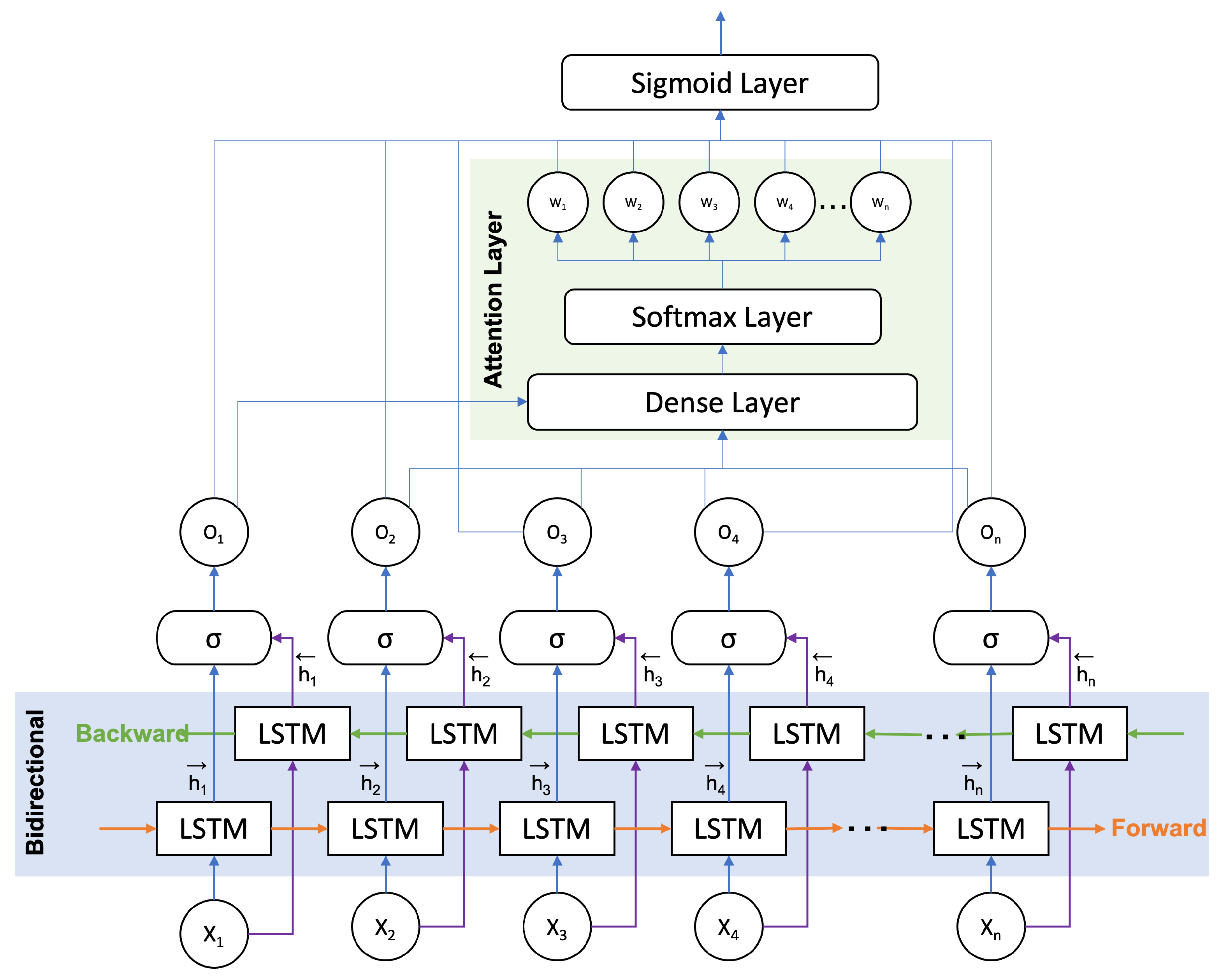
- Utilizes a bidirectional LSTM to encode the historical meteorological and tide data sequence into a vector and subsequently decodes the vector with weights derived from the attention layer to make the prediction.
- 2.
- Explores the integration of an attention mechanism to enhance prediction accuracy by extracting meteorological, tidal, and typhoon features of storm surge time series and using them as input to the model.
- 3.
- In contrast to traditional numerical weather prediction models, BALSSA can handle non-stationary sequences and capture all non-linear interactions more effectively [18].
- 4.
- Compared to other deep learning models, BALSSA has superior interpretability and can avoid the long-term dependence issues [19].
- 1.
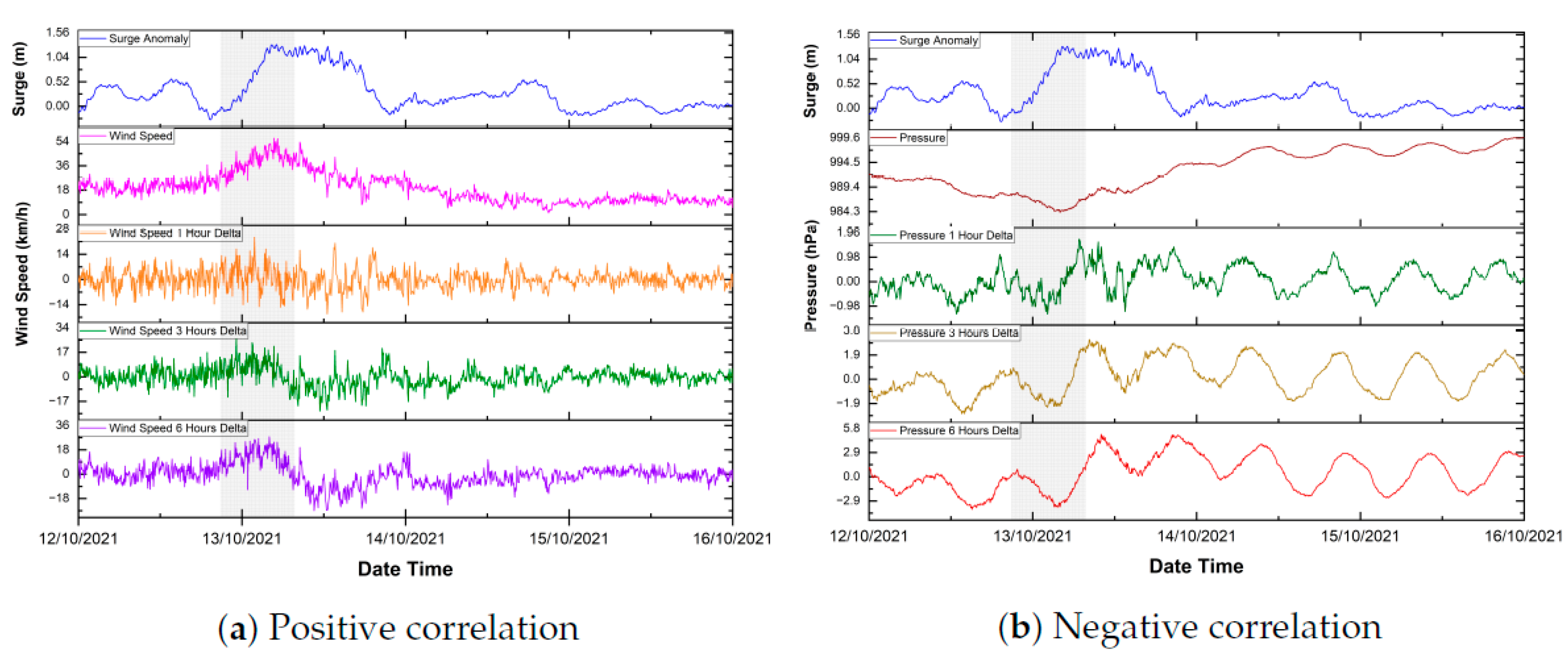
- The model focuses on specific features of the data that are most relevant for making accurate predictions. For instance, in storm surge prediction, it can identify which weather variables (such as wind speed, air pressure, and temperature) are most influential in determining the likelihood and severity of a surge.
- 2.
- The model captures complex relationships between the weather variables that may not be apparent from simple statistical analysis. For example, it can help the model recognize how changes in one variable (such as wind speed) can affect other variables (such as water level or wave height) and how these changes can combine to create a storm surge.
- 3.
- The model handles non-linear and non-stationary relationships between the weather variables, which can be difficult for traditional statistical models. It captures the dynamic interactions between the weather variables and adjusts their weights based on the current state of the system, allowing them to adapt to ever-changing weather conditions and make more accurate predictions.
2. Related Works
3. Model Architecture
3.1. Model Structure
3.1.1. Bidirectional LSTM Layer
3.1.2. Attention Layer
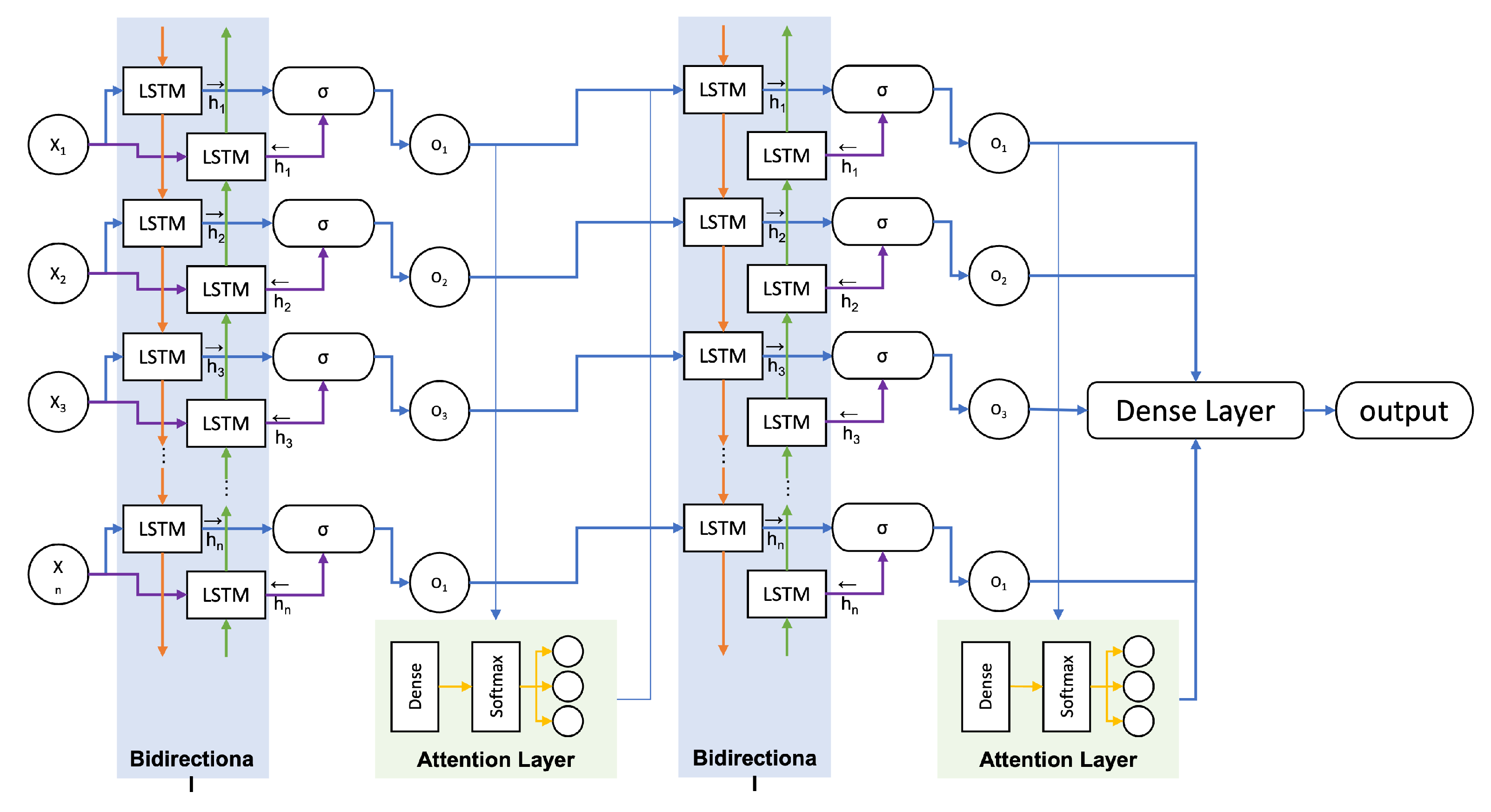
3.1.3. Dual-BALSSA, D-BALSSA
- Enhanced management of complex relationships: Accurate storm surge prediction requires modeling the complex relationships between various factors, such as wind speed, sea level, and atmospheric pressure. The dual-layer design of D-BALSSA helps capture these complex correlations and long-term dependencies, leading to more accurate predictions.
- Improved feature selection: The prediction of storm surges involves analyzing complex relationships between multiple factors, such as wind speed, sea level, and atmospheric pressure. The architecture of D-BALSSA effectively captures these relationships and improves its ability to identify and incorporate important information into its predictions, leading to more accurate results.
3.2. Data Collection and Preprocessing
3.2.1. Data Collection
3.2.2. Data Preprocessing and Imputation
3.3. Model Evaluation Metrics
4. Result Analysis
5. Discussion
5.1. The Unpredictability of Storm Surge
5.2. Appropriate ML Models
5.3. Advantages over Traditional Methods for Handling Uncertainty
6. Final Remarks and Future Work
Author Contributions
Funding
Institutional Review Board Statement
Informed Consent Statement
Data Availability Statement
Acknowledgments
Conflicts of Interest
References
- Conner, W.; Kraft, R.; Harris, D.L. Empirical methods for forecasting the maximum storm tide due to hurricanes and other tropical storms. Mon. Weather Rev. 1957, 85, 113–116. [Google Scholar] [CrossRef]
- Nicholls, R.J.; Cazenave, A. Sea-level rise and its impact on coastal zones. Science 2010, 328, 1517–1520. [Google Scholar] [CrossRef] [PubMed]
- Emanuel, K. Increasing destructiveness of tropical cyclones over the past 30 years. Nature 2005, 436, 686–688. [Google Scholar] [CrossRef] [PubMed]
- Heaps, N. Storm surges, 1967–1982. Geophys. J. Int. 1983, 74, 331–376. [Google Scholar] [CrossRef] [Green Version]
- Marsooli, R.; Lin, N. Numerical modeling of historical storm tides and waves and their interactions along the US East and Gulf Coasts. J. Geophys. Res. Ocean. 2018, 123, 3844–3874. [Google Scholar] [CrossRef] [Green Version]
- Jin, X.; Shi, X.; Gao, J.; Xu, T.; Yin, K. Evaluation of loss due to storm surge disasters in China based on econometric model groups. Int. J. Environ. Res. Public Health 2018, 15, 604. [Google Scholar] [CrossRef] [Green Version]
- Ian, V.K.; Tse, R.; Tang, S.K.; Pau, G. Performance Analysis of Machine Learning Algorithms in Storm Surge Prediction. In Proceedings of the IoTBDS, Online Streaming, 22–24 April 2022; pp. 297–303. [Google Scholar]
- Hoover, R.A. Empirical relationships of the central pressures in hurricanes to the maximum surge and storm tide. Mon. Weather Rev. 1957, 85, 167–174. [Google Scholar] [CrossRef]
- Welander, P. Numerical prediction of storm surges. In Advances in Geophysics; Elsevier: Amsterdam, The Netherlands, 1961; Volume 8, pp. 315–379. [Google Scholar]
- Kohno, N.; Dube, S.K.; Entel, M.; Fakhruddin, S.; Greenslade, D.; Leroux, M.D.; Rhome, J.; Thuy, N.B. Recent progress in storm surge forecasting. Trop. Cyclone Res. Rev. 2018, 7, 128–139. [Google Scholar]
- Wang, Z.; Zhou, L.; Li, Q.; Sun, X. Storm surge along the Yellow River Delta under directional extreme wind conditions. J. Coast. Res. 2017, 9, 86–91. [Google Scholar] [CrossRef]
- Xie, K.; Ozbay, K.; Zhu, Y.; Yang, H. Evacuation zone modeling under climate change: A data-driven method. J. Infrastruct. Syst. 2017, 23, 04017013. [Google Scholar] [CrossRef]
- Suleman, M.A.R.; Shridevi, S. Short-Term Weather Forecasting Using Spatial Feature Attention Based LSTM Model. IEEE Access 2022, 10, 82456–82468. [Google Scholar] [CrossRef]
- Kim, S.; Matsumi, Y.; Pan, S.; Mase, H. A real-time forecast model using artificial neural network for after-runner storm surges on the Tottori coast, Japan. Ocean Eng. 2016, 122, 44–53. [Google Scholar] [CrossRef]
- Lee, T.L. Neural network prediction of a storm surge. Ocean Eng. 2006, 33, 483–494. [Google Scholar] [CrossRef]
- Jan, C.D.; Tseng, C.M.; Wang, J.S.; Cheng, Y.H. Empirical relation between the typhoon surge deviation and the corresponding typhoon characteristics: A case study in Taiwan. J. Mar. Sci. Technol. 2006, 11, 193–200. [Google Scholar] [CrossRef]
- Wu, G.; Shi, F.; Kirby, J.T.; Liang, B.; Shi, J. Modeling wave effects on storm surge and coastal inundation. Coast. Eng. 2018, 140, 371–382. [Google Scholar] [CrossRef]
- Pitt, M. Learning Lessons from the 2007 Floods; Pitt Review; Dalhousie University: Halifax, NS, Canada, 2008. [Google Scholar]
- Ian, V.K.; Tse, R.; Tang, S.K.; Pau, G. Novel Prediction in Storm Surge Using Ensemble Machine Learning Algorithms. In Proceedings of the 2022 5th International Conference on Pattern Recognition and Artificial Intelligence (PRAI), Chengdu, China, 19–21 August 2022; pp. 1229–1234. [Google Scholar]
- Tsai, C.P.; You, C.Y. Development of models for maximum and time variation of storm surges at the Tanshui estuary. Nat. Hazards Earth Syst. Sci. 2014, 14, 2313–2320. [Google Scholar] [CrossRef] [Green Version]
- Borah, D.K. Hydrologic procedures of storm event watershed models: A comprehensive review and comparison. Hydrol. Process. 2011, 25, 3472–3489. [Google Scholar] [CrossRef]
- Costabile, P.; Costanzo, C.; Macchione, F. A storm event watershed model for surface runoff based on 2D fully dynamic wave equations. Hydrol. Process. 2013, 27, 554–569. [Google Scholar] [CrossRef]
- Nayak, P.; Sudheer, K.; Rangan, D.; Ramasastri, K. Short-term flood forecasting with a neurofuzzy model. Water Resour. Res. 2005, 41. [Google Scholar] [CrossRef] [Green Version]
- Kim, B.; Sanders, B.F.; Famiglietti, J.S.; Guinot, V. Urban flood modeling with porous shallow-water equations: A case study of model errors in the presence of anisotropic porosity. J. Hydrol. 2015, 523, 680–692. [Google Scholar] [CrossRef] [Green Version]
- Van den Honert, R.C.; McAneney, J. The 2011 Brisbane floods: Causes, impacts and implications. Water 2011, 3, 1149–1173. [Google Scholar] [CrossRef] [Green Version]
- Bode, L.; Hardy, T.A. Progress and recent developments in storm surge modeling. J. Hydraul. Eng. 1997, 123, 315–331. [Google Scholar] [CrossRef]
- Heemink, A.W.; Bolding, K.; Verlaan, M. Storm Surge Forecasting Using Kalman Filtering: A Review; Citeseer: Princeton, NJ, USA, 1995. [Google Scholar]
- Battjes, J.A.; Gerritsen, H. Coastal modelling for flood defence. Philos. Trans. R. Soc. Lond. Ser. A Math. Phys. Eng. Sci. 2002, 360, 1461–1475. [Google Scholar] [CrossRef] [PubMed]
- Verlaan, M.; Zijderveld, A.; de Vries, H.; Kroos, J. Operational storm surge forecasting in the Netherlands: Developments in the last decade. Philos. Trans. R. Soc. A Math. Phys. Eng. Sci. 2005, 363, 1441–1453. [Google Scholar] [CrossRef]
- Shrestha, D.; Robertson, D.; Wang, Q.; Pagano, T.; Hapuarachchi, H. Evaluation of numerical weather prediction model precipitation forecasts for short-term streamflow forecasting purpose. Hydrol. Earth Syst. Sci. 2013, 17, 1913–1931. [Google Scholar] [CrossRef] [Green Version]
- Mosavi, A.; Rabczuk, T.; Varkonyi-Koczy, A.R. Reviewing the novel machine learning tools for materials design. In Proceedings of the International Conference on Global Research and Education, Kaunas, Lithuania, 24–27 September 2018; pp. 50–58. [Google Scholar]
- Abbot, J.; Marohasy, J. Input selection and optimisation for monthly rainfall forecasting in Queensland, Australia, using artificial neural networks. Atmos. Res. 2014, 138, 166–178. [Google Scholar] [CrossRef]
- Merz, B.; Hall, J.; Disse, M.; Schumann, A. Fluvial flood risk management in a changing world. Nat. Hazards Earth Syst. Sci. 2010, 10, 509–527. [Google Scholar] [CrossRef] [Green Version]
- Xu, Z.; Li, J. Short-term inflow forecasting using an artificial neural network model. Hydrol. Process. 2002, 16, 2423–2439. [Google Scholar] [CrossRef]
- Lee, T.L. Predictions of typhoon storm surge in Taiwan using artificial neural networks. Adv. Eng. Softw. 2009, 40, 1200–1206. [Google Scholar] [CrossRef]
- Quinn, N.; Lewis, M.; Wadey, M.; Haigh, I. Assessing the temporal variability in extreme storm-tide time series for coastal flood risk assessment. J. Geophys. Res. Ocean. 2014, 119, 4983–4998. [Google Scholar] [CrossRef] [Green Version]
- Doycheva, K.; Horn, G.; Koch, C.; Schumann, A.; König, M. Assessment and weighting of meteorological ensemble forecast members based on supervised machine learning with application to runoff simulations and flood warning. Adv. Eng. Inform. 2017, 33, 427–439. [Google Scholar] [CrossRef] [Green Version]
- Fleming, S.W.; Bourdin, D.R.; Campbell, D.; Stull, R.B.; Gardner, T. Development and operational testing of a super-ensemble artificial intelligence flood-forecast model for a Pacific Northwest river. JAWRA J. Am. Water Resour. Assoc. 2015, 51, 502–512. [Google Scholar] [CrossRef]
- Feng, X.; Li, M.; Yin, B.; Yang, D.; Yang, H. Study of storm surge trends in typhoon-prone coastal areas based on observations and surge-wave coupled simulations. Int. J. Appl. Earth Obs. Geoinf. 2018, 68, 272–278. [Google Scholar] [CrossRef]
- Kim, G.; Barros, A.P. Quantitative flood forecasting using multisensor data and neural networks. J. Hydrol. 2001, 246, 45–62. [Google Scholar] [CrossRef]
- Danso-Amoako, E.; Scholz, M.; Kalimeris, N.; Yang, Q.; Shao, J. Predicting dam failure risk for sustainable flood retention basins: A generic case study for the wider Greater Manchester area. Comput. Environ. Urban Syst. 2012, 36, 423–433. [Google Scholar] [CrossRef]
- Saghafian, B.; Haghnegahdar, A.; Dehghani, M. Effect of ENSO on annual maximum floods and volume over threshold in the southwestern region of Iran. Hydrol. Sci. J. 2017, 62, 1039–1049. [Google Scholar] [CrossRef]
- Kourgialas, N.N.; Dokou, Z.; Karatzas, G.P. Statistical analysis and ANN modeling for predicting hydrological extremes under climate change scenarios: The example of a small Mediterranean agro-watershed. J. Environ. Manag. 2015, 154, 86–101. [Google Scholar] [CrossRef]
- Sahoo, B.; Bhaskaran, P.K. Prediction of storm surge and coastal inundation using Artificial Neural Network–A case study for 1999 Odisha Super Cyclone. Weather Clim. Extrem. 2019, 23, 100196. [Google Scholar] [CrossRef]
- Wang, B.; Liu, S.; Wang, B.; Wu, W.; Wang, J.; Shen, D. Multi-step ahead short-term predictions of storm surge level using CNN and LSTM network. Acta Oceanol. Sin. 2021, 40, 104–118. [Google Scholar] [CrossRef]
- Xie, J.; Zhang, J.; Yu, J.; Xu, L. An adaptive scale sea surface temperature predicting method based on deep learning with attention mechanism. IEEE Geosci. Remote Sens. Lett. 2019, 17, 740–744. [Google Scholar] [CrossRef]
- Luo, Q.R.; Xu, H.; Bai, L.H. Prediction of significant wave height in hurricane area of the Atlantic Ocean using the Bi-LSTM with attention model. Ocean Eng. 2022, 266, 112747. [Google Scholar] [CrossRef]
- Cheng, Q.; Li, H.; Wu, Q.; Meng, F.; Xu, L.; Ngan, K.N. Learn to pay attention via switchable attention for image recognition. In Proceedings of the 2020 IEEE Conference on Multimedia Information Processing and Retrieval (MIPR), Shenzhen, China, 6–8 August 2020; pp. 291–296. [Google Scholar]
- Luong, M.T.; Pham, H.; Manning, C.D. Effective approaches to attention-based neural machine translation. arXiv 2015, arXiv:1508.04025. [Google Scholar]
- Li, Q.; Zhu, Y.; Shangguan, W.; Wang, X.; Li, L.; Yu, F. An attention-aware LSTM model for soil moisture and soil temperature prediction. Geoderma 2022, 409, 115651. [Google Scholar] [CrossRef]
- Qin, Y.; Song, D.; Chen, H.; Cheng, W.; Jiang, G.; Cottrell, G. A dual-stage attention-based recurrent neural network for time series prediction. arXiv 2017, arXiv:1704.02971. [Google Scholar]
- Liu, Y.; Gong, C.; Yang, L.; Chen, Y. DSTP-RNN: A dual-stage two-phase attention-based recurrent neural network for long-term and multivariate time series prediction. Expert Syst. Appl. 2020, 143, 113082. [Google Scholar] [CrossRef]
- Gangopadhyay, T.; Tan, S.Y.; Jiang, Z.; Meng, R.; Sarkar, S. Spatiotemporal attention for multivariate time series prediction and interpretation. In Proceedings of the ICASSP 2021–2021 IEEE International Conference on Acoustics, Speech and Signal Processing (ICASSP), Toronto, ON, Canada, 6–11 June 2021; pp. 3560–3564. [Google Scholar]
- Shi, L.; Liang, N.; Xu, X.; Li, T.; Zhang, Z. SA-JSTN: Self-attention joint spatiotemporal network for temperature forecasting. IEEE J. Sel. Top. Appl. Earth Obs. Remote Sens. 2021, 14, 9475–9485. [Google Scholar] [CrossRef]
- HOLLAND, G. An Analytic Model of the Wind and Pressure Profiles in Hurricanes. Mon. Weather Rev. 1980, 108, 1212–1218. [Google Scholar] [CrossRef]
- Das, Y.; Mohanty, U.; Jain, I. Development of tropical cyclone wind field for simulation of storm surge/sea surface height using numerical ocean model. Model. Earth Syst. Environ. 2016, 2, 1–22. [Google Scholar] [CrossRef] [Green Version]
- De Oliveira, M.M.; Ebecken, N.F.F.; De Oliveira, J.L.F.; de Azevedo Santos, I. Neural network model to predict a storm surge. J. Appl. Meteorol. Climatol. 2009, 48, 143–155. [Google Scholar] [CrossRef]
- Lee, T.L. Back-propagation neural network for long-term tidal predictions. Ocean Eng. 2004, 31, 225–238. [Google Scholar] [CrossRef]
- Sztobryn, M. Forecast of storm surge by means of artificial neural network. J. Sea Res. 2003, 49, 317–322. [Google Scholar] [CrossRef]
- Kim, S.; Pan, S.; Mase, H. Artificial neural network-based storm surge forecast model: Practical application to Sakai Minato, Japan. Appl. Ocean Res. 2019, 91, 101871. [Google Scholar] [CrossRef]
- Tseng, C.M.; Jan, C.D.; Wang, J.S.; Wang, C. Application of artificial neural networks in typhoon surge forecasting. Ocean Eng. 2007, 34, 1757–1768. [Google Scholar] [CrossRef]
- HKO. Hong Kong Observatory Open Data. Available online: https://www.hko.gov.hk/en/abouthko/opendata_intro.htm (accessed on 8 December 2022).
- SMG. Macao Meteorological and Geophysical Bureau. Available online: https://www.smg.gov.mo/en (accessed on 28 December 2022).
- Huang, Y.H.; Wu, C.C.; Wang, Y. The influence of island topography on typhoon track deflection. Mon. Weather Rev. 2011, 139, 1708–1727. [Google Scholar] [CrossRef]
- Westerink, J.J.; Luettich, R.A.; Baptists, A.; Scheffner, N.W.; Farrar, P. Tide and storm surge predictions using finite element model. J. Hydraul. Eng. 1992, 118, 1373–1390. [Google Scholar] [CrossRef]
- Liu, W.C.; Huang, W.C.; Chen, W.B. Modeling the interaction between tides and storm surges for the Taiwan coast. Environ. Fluid Mech. 2016, 16, 721–745. [Google Scholar] [CrossRef]
- Lin, N.; Chavas, D. On hurricane parametric wind and applications in storm surge modeling. J. Geophys. Res. Atmos. 2012, 117. [Google Scholar] [CrossRef]
- Olfateh, M.; Callaghan, D.P.; Nielsen, P.; Baldock, T.E. Tropical cyclone wind field asymmetry—Development and evaluation of a new parametric model. J. Geophys. Res. Ocean. 2017, 122, 458–469. [Google Scholar] [CrossRef] [Green Version]
- Jones, J.E.; Davies, A.M. Influence of non-linear effects upon surge elevations along the west coast of Britain. Ocean Dyn. 2007, 57, 401–416. [Google Scholar] [CrossRef]
- Bajo, M.; Umgiesser, G. Storm surge forecast through a combination of dynamic and neural network models. Ocean Model. 2010, 33, 1–9. [Google Scholar] [CrossRef]
- Erdil, A.; Arcaklioglu, E. The prediction of meteorological variables using artificial neural network. Neural Comput. Appl. 2013, 22, 1677–1683. [Google Scholar] [CrossRef]
- Chen, W.B.; Liu, W.C.; Hsu, M.H. Computational investigation of typhoon-induced storm surges along the coast of Taiwan. Nat. Hazards 2012, 64, 1161–1185. [Google Scholar] [CrossRef]
- Chen, W.B.; Lin, L.Y.; Jang, J.H.; Chang, C.H. Simulation of typhoon-induced storm tides and wind waves for the northeastern coast of Taiwan using a tide–surge–wave coupled model. Water 2017, 9, 549. [Google Scholar] [CrossRef] [Green Version]
- Dietrich, J.; Muhammad, A.; Curcic, M.; Fathi, A.; Dawson, C.; Chen, S.S.; Luettich, R., Jr. Sensitivity of storm surge predictions to atmospheric forcing during Hurricane Isaac. J. Waterw. Port Coast. Ocean Eng. 2018, 144, 04017035. [Google Scholar] [CrossRef]
- Liu, Q.; Ruan, C.; Zhong, S.; Li, J.; Yin, Z.; Lian, X. Risk assessment of storm surge disaster based on numerical models and remote sensing. Int. J. Appl. Earth Obs. Geoinf. 2018, 68, 20–30. [Google Scholar] [CrossRef]
- Torres, M.J.; Reza Hashemi, M.; Hayward, S.; Spaulding, M.; Ginis, I.; Grilli, S.T. Role of hurricane wind models in accurate simulation of storm surge and waves. J. Waterw. Port Coast. Ocean Eng. 2019, 145, 04018039. [Google Scholar] [CrossRef]
- Dismukes, D.E.; Narra, S. Sea-Level Rise and Coastal Inundation: A Case Study of the Gulf Coast Energy Infrastructure. Nat. Resour. 2018, 9, 150–174. [Google Scholar] [CrossRef] [Green Version]
- Webster, P.J.; Holland, G.J.; Curry, J.A.; Chang, H.R. Changes in tropical cyclone number, duration, and intensity in a warming environment. Science 2005, 309, 1844–1846. [Google Scholar] [CrossRef] [Green Version]


| Date Time | Predicted Tide (m) | Actual Tide (m) | P # (hPa) | Wind Dir | WS * (km/h) | WS * 1 h Delta (km/h) | P # 1 h Delta (hPa) |
|---|---|---|---|---|---|---|---|
| 1 January 2021 0:00 | 2.61 | 3.084 | 1013.6 | NNE | 18.36 | −6.48 | 0.3 |
| 1 January 2021 0:05 | 2.58 | 3.084 | 1013.6 | NNE | 19.08 | 1.80 | 0.3 |
| 1 January 2021 0:10 | 2.55 | 3.089 | 1013.6 | NE | 17.28 | −8.64 | 0.4 |
| 1 January 2021 0:15 | 2.53 | 3.085 | 1013.7 | NNE | 15.84 | 0.555 | 0.6 |
| 1 January 2021 0:20 | 2.50 | 3.050 | 1013.6 | NNE | 14.40 | −5.40 | 0.4 |
| 1 January 2021 0:25 | 2.47 | 3.016 | 1013.7 | NNE | 16.20 | −8.28 | 0.5 |
| 1 January 2021 0:30 | 2.44 | 2.952 | 1013.7 | NNE | 18.36 | 5.040 | 0.4 |
| Features of Wind and Pressure Tendency | ||||
|---|---|---|---|---|
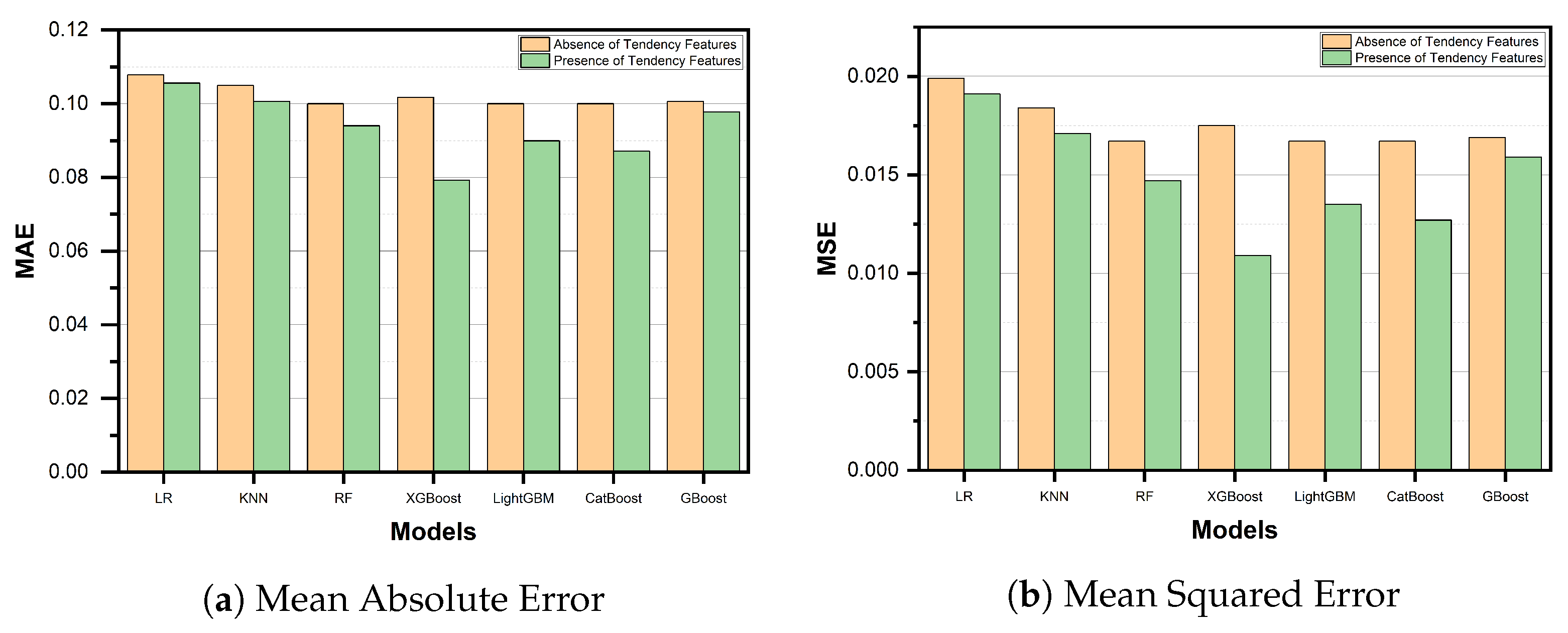
| Model | Metric | Stage | Absence | Presence |
| Linear Regression | MAE | Train | 0.1071 | 0.1048 |
| Val | 0.1073 | 0.1052 | ||
| Test | 0.1078 | 0.1056 | ||
| MSE | Train | 0.0195 | 0.0187 | |
| Val | 0.0198 | 0.0191 | ||
| Test | 0.0199 | 0.0191 | ||
| K-Nearest Neighbor | MAE | Train | 0.0936 | 0.0903 |
| Val | 0.1033 | 0.1000 | ||
| Test | 0.1049 | 0.1006 | ||
| MSE | Train | 0.0146 | 0.0136 | |
| Val | 0.0178 | 0.0168 | ||
| Test | 0.0184 | 0.0171 | ||
| Random Forest | MAE | Train | 0.0967 | 0.0904 |
| Val | 0.0983 | 0.0929 | ||
| Test | 0.1000 | 0.0940 | ||
| MSE | Train | 0.0154 | 0.0134 | |
| Val | 0.0162 | 0.0144 | ||
| Test | 0.0167 | 0.0147 | ||
| XGBoost | MAE | Train | 0.0802 | 0.0435 |
| Val | 0.1005 | 0.0779 | ||
| Test | 0.1017 | 0.0792 | ||
| MSE | Train | 0.0109 | 0.0036 | |
| Val | 0.0171 | 0.0104 | ||
| Test | 0.0175 | 0.0109 | ||
| LightGBM | MAE | Train | 0.0958 | 0.0838 |
| Val | 0.0984 | 0.0886 | ||
| Test | 0.1000 | 0.0899 | ||
| MSE | Train | 0.0151 | 0.0115 | |
| Val | 0.0162 | 0.0131 | ||
| Test | 0.0167 | 0.0135 | ||
| CatBoost | MAE | Train | 0.0958 | 0.0774 |
| Val | 0.0984 | 0.0856 | ||
| Test | 0.1000 | 0.0871 | ||
| MSE | Train | 0.0151 | 0.0099 | |
| Val | 0.0162 | 0.0122 | ||
| Test | 0.0167 | 0.0127 | ||
| Gradient Boosting | MAE | Train | 0.0992 | 0.0960 |
| Val | 0.0991 | 0.0967 | ||
| Test | 0.1006 | 0.0977 | ||
| MSE | Train | 0.0163 | 0.0152 | |
| Val | 0.0163 | 0.0155 | ||
| Test | 0.0169 | 0.0159 | ||
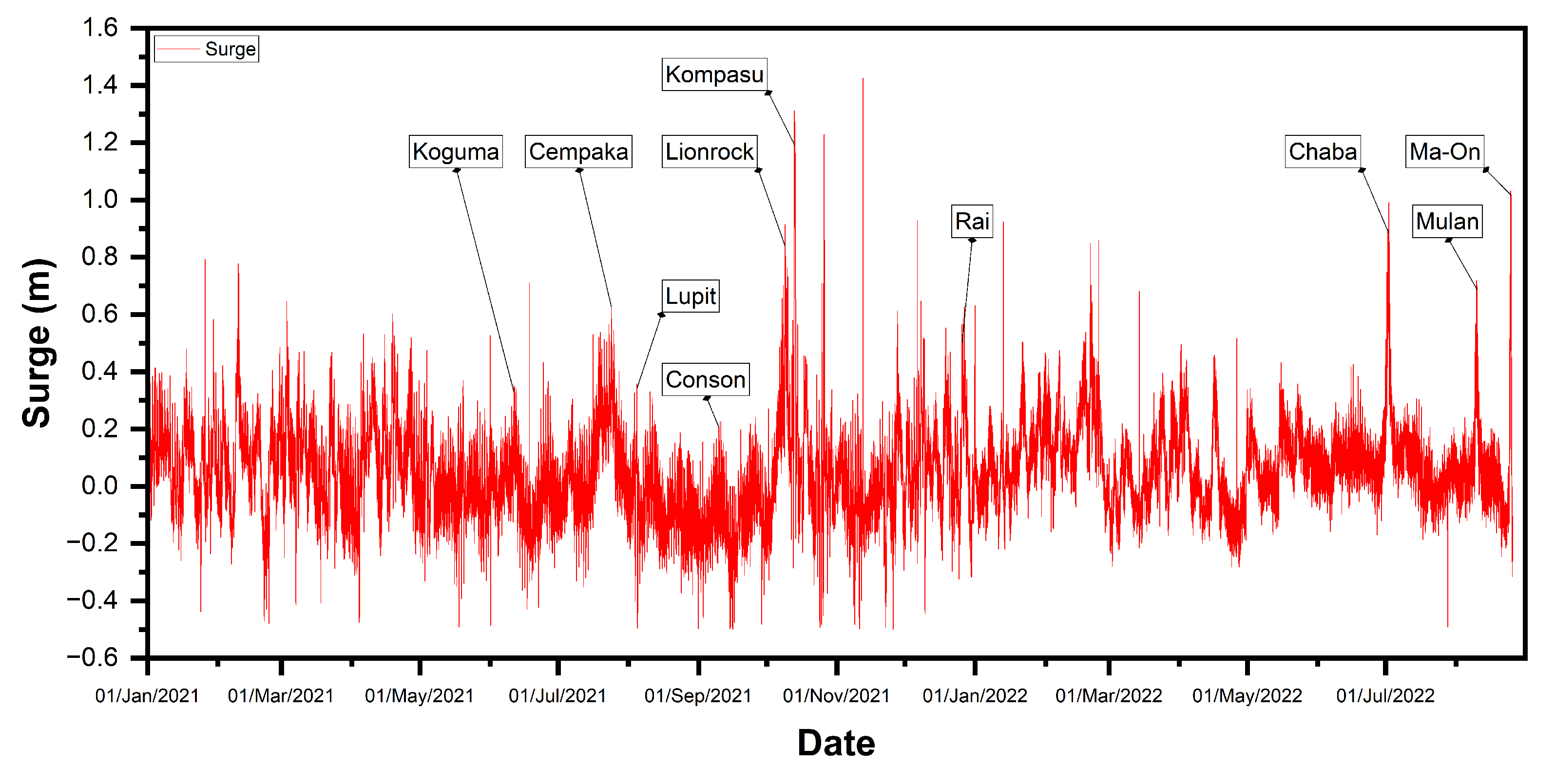
| TC | Name | Duration | Grade | Highest Wind (km/h) | Lowest Pressure (hPa) |
|---|---|---|---|---|---|
| 1 | Koguma | 6 November–6 December 2021 | Tropical Storm | 65 | 996 |
| 2 | Cempaka | 18 July–21 July 2021 | Typhoon | 130 | 980 |
| 3 | Lupit | 2–4 August 2021 | Tropical Storm | 85 | 984 |
| 4 | Conson | 9–10 September 2021 | Severe Tropical Storm | 95 | 992 |
| 5 | Lionrock | 7–10 October 2021 | Tropical Storm | 65 | 994 |
| 6 | Kompasu | 11–14 October 2021 | Typhoon | 100 | 975 |
| 7 | Rai | 20–21 December 2021 | Super Typhoon | 195 | 915 |
| 8 | Chaba | 29 June–3 July 2022 | Typhoon | 130 | 965 |
| 9 | Mulan | 9–11 August 2022 | Tropical storm | 65 | 994 |
| 10 | Ma-On | 23–25 August 2022 | Typhoon | 100 | 980 |
| Classification | Abbreviation | Maximum Sustained Winds Near the Center (km/h) |
|---|---|---|
| Tropical Depression | TD | 41–62 |
| Tropical Storm | TS | 63–87 |
| Severe Tropical Storm | STS | 88–117 |
| Typhoon | T | 118–149 |
| Severe Typhoon | ST | 150–184 |
| Super Typhoon | SuperT | 185 or above |
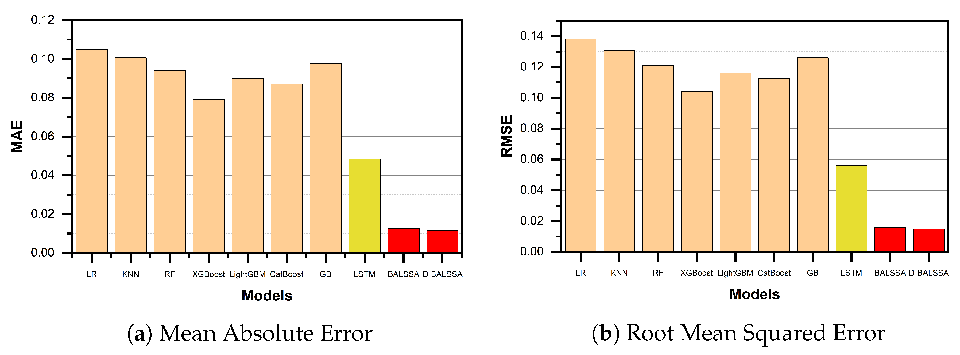
| Metric | LR | KNN | RF | XGBoost | LightGBM | CatBoost | GB | LSTM | BALSSA | D-BALSSA |
|---|---|---|---|---|---|---|---|---|---|---|
| MAE | 0.1050 | 0.1006 | 0.0940 | 0.0792 | 0.0899 | 0.0871 | 0.0977 | 0.0484 | 0.0126 | 0.0114 |
| MSE | 0.0191 | 0.0171 | 0.0147 | 0.0109 | 0.0135 | 0.0127 | 0.0159 | 0.0032 | 0.0003 | 0.0002 |
| RMSE | 0.1382 | 0.1308 | 0.1211 | 0.1043 | 0.1161 | 0.1126 | 0.1260 | 0.0560 | 0.0159 | 0.0147 |
Disclaimer/Publisher’s Note: The statements, opinions and data contained in all publications are solely those of the individual author(s) and contributor(s) and not of MDPI and/or the editor(s). MDPI and/or the editor(s) disclaim responsibility for any injury to people or property resulting from any ideas, methods, instructions or products referred to in the content. |
© 2023 by the authors. Licensee MDPI, Basel, Switzerland. This article is an open access article distributed under the terms and conditions of the Creative Commons Attribution (CC BY) license (https://creativecommons.org/licenses/by/4.0/).
Share and Cite
Ian, V.-K.; Tse, R.; Tang, S.-K.; Pau, G. Bridging the Gap: Enhancing Storm Surge Prediction and Decision Support with Bidirectional Attention-Based LSTM. Atmosphere 2023, 14, 1082. https://doi.org/10.3390/atmos14071082
Ian V-K, Tse R, Tang S-K, Pau G. Bridging the Gap: Enhancing Storm Surge Prediction and Decision Support with Bidirectional Attention-Based LSTM. Atmosphere. 2023; 14(7):1082. https://doi.org/10.3390/atmos14071082
Chicago/Turabian StyleIan, Vai-Kei, Rita Tse, Su-Kit Tang, and Giovanni Pau. 2023. "Bridging the Gap: Enhancing Storm Surge Prediction and Decision Support with Bidirectional Attention-Based LSTM" Atmosphere 14, no. 7: 1082. https://doi.org/10.3390/atmos14071082