Article

The Role of Water Vapor Observations in Satellite Rainfall Detection Highlighted by a Deep Learning Approach

by
Mónica Estébanez-Camarena
*,†,
Fabio Curzi
,
Riccardo Taormina
,
Nick van de Giesen
and
Marie-Claire ten Veldhuis
Faculty of Civil Engineering and Geosciences, Delft University of Technology, 2628 CN Delft, The Netherlands
*
Author to whom correspondence should be addressed.
These authors contributed equally to this work.
Atmosphere 2023, 14(6), 974; https://doi.org/10.3390/atmos14060974
Submission received: 12 April 2023 / Revised: 25 May 2023 / Accepted: 30 May 2023 / Published: 2 June 2023
(This article belongs to the Special Issue Precipitation in Africa)

Abstract

:
West African food systems and rural socio-economics are based on rainfed agriculture, which makes society highly vulnerable to rainfall uncertainty and frequent floods and droughts. Reliable rainfall information is currently missing. There is a sparse and uneven rain gauge distribution and, despite continuous efforts, rainfall satellite products continue to show weak correlations with ground measurements. This paper aims to investigate whether water vapor (WV) observations together with temporal information can complement thermal infrared (TIR) data for satellite rainfall retrieval in a Deep Learning (DL) framework. This is motivated by the fact that water vapor plays a key role in the highly seasonal West African rainfall dynamics. We present a DL model for satellite rainfall detection based on WV and TIR channels of Meteosat Second Generation and temporal information. Results show that the WV inhibition of low-level features enables the depiction of strong convective motions usually related to heavy rainfall. This is especially relevant in areas where convective rainfall is dominant, such as the tropics. Additionally, WV data allow us to detect dry air masses over our study area, that are advected from the Sahara Desert and create discontinuities in precipitation events. The developed DL model shows strong performance in rainfall binary classification, with less false alarms and lower rainfall overdetection (FBias < 2.0 ) than the state-of-the-art Integrated MultisatellitE Retrievals for GPM (IMERG) Final Run.

1. Introduction

In West Africa, rainfed agriculture is the main pillar of the food system and rural socio-economics. For example, in Ghana, the focus area of this study, agriculture accounts for 54% of the total Gross Domestic Product [1] and is predominantly rainfed small-holder farming. Rainfall in this area is highly uncertain and there are frequent floods and droughts, exacerbated by climate change. Reliable and timely rainfall information is essential to effectively face these challenges and avoid major economic and yield losses. However, a sparse and unevenly distributed rain gauge network—as is typical for tropical areas [2,3]—and regionally poor-performing satellite rainfall products, hinder the availability of accurate dense rainfall information.
The global coverage of Earth observation satellites can offer a solution for poorly ground-monitored areas. The most widely used methodologies for satellite rainfall retrieval are based on thermal infrared (TIR) from Geostationary (GEO) satellites and passive microwave (PMW) data from Low-Earth Orbit (LEO) satellites. Because of their closer proximity to the Earth’s surface, LEO satellites allow for a higher spatial resolution but have the disadvantage of a longer revisit time, which often translates to rainfall events being missed. On the contrary, GEO satellites provide a lower spatial resolution but have the advantage of a constant view of the full Earth disk from their unique position, always above the same point above the Earth’s surface. This enables them to have a high temporal resolution and to monitor atmospheric processes like no other satellite platform. This will only become more apparent with Meteosat Third Generation, for which the first satellite has recently been launched [4]. Retrieval methods can be physical- or Machine Learning-based, or a combination of both. Within Machine Learning, Deep Larning (DL) aims to minimize human intervention and facilitate automated feature extraction from large raw datasets [5]. This new data-oriented approach is a promising method to detect and possibly estimate rainfall when theoretical or process-based approaches fail to accurately parameterize such complex atmospheric processes.
Physical-based retrieval methods that use TIR data predominantly employ the Cold Cloud Duration (CCD) method, which correlates the time that a pixel is under a certain temperature threshold with rainfall on the ground. Two examples of this approach are the Tropical Applications of Meteorology Using Satellite Data and Ground-Based Observations (TAMSAT) [6] and the Africa Climate Hazards Infrared Precipitation with Stations (CHIRPS) [7] rainfall products, specifically designed for Africa with daily and 6-hourly temporal resolutions, respectively. Results from a calibration of the CCD method in the Sahel region are unreliable due to spatial averaging and temporal aggregation, as well as low gauge density [8]. In West Africa, both TAMSAT and CHIRPS show daily Kling–Gupta Efficiency values below 0.4 [9,10].
To address the limitations of the CCD method and exploit the benefits of DL, ref. [11] developed a novel DL-based methodology: RainRunner. RainRunner classifies 3 h intervals into rain/no-rain, based only on TIR data. Rainrunner was trained over the North of Ghana using rain gauge data as target, with a very small training dataset—measurements from 8 rain gauges over 2.5 years—with TIR data as the only input and based on standard DL architectures. Nonetheless, this approach showed promising results, reaching near state-of-the-art performances. However, as expected for methods that rely only on TIR data [12], RainRunner heavily overdetected rainfall.
PMW sensors allow for a more direct retrieval of rainfall than TIR sensors because they directly sense hydrometeors in the atmosphere. Using this advantage, the Global Precipitation Measurement (GPM) Integrated Multisatellite Retrievals for GPM (IMERG) rainfall product combines data from TIR and PMW sensors, along with atmospheric reanalysis and rain gauge data. Developed by NASA through the use of physical- and Machine Learning-based algorithms, IMERG aims to become the longest and most detailed rainfall dataset available [13]. Compared with other regions of the world, IMERG shows a weaker correlation with ground measurements in West Africa [14,15].
The literature suggests that the poor regional performance of satellite rainfall products over West Africa is partly due to sparse rain gauge coverage [8], as has also been observed in other regions of the world [16]. Another reason for this poor performance is the complexity of West African rainfall dynamics. They are governed by the seasonal northward shift of the Intertropical Convergence Zone (ITCZ) and the West African Monsoon (WAM), a low-level south westerly moist flow from the Atlantic Ocean. Wind shear generated by the monsoonal flow creates a strong temperature contrast—especially from June to September—between the dry hot Sahara Desert and the cool moist Guinea coast that favors the formation of the African Easterly Jet. The African Easterly Jet is a unique zonal wind feature located in the midlevel troposphere around 600 hPa (Figure 1) and is most intense at the end of August. The jet is caused by a thermal wind balance that promotes the development of the African Easterly waves (AEWs) through baroclinic and barotropic instability [2]. Many studies [17,18,19] have identified water vapor as a key factor in West African rainfall dynamics. Studies have shown that the main support for the intensification of AEWs is moist convection. At the same time, latent heat release from condensation of atmospheric water vapor and a strong solar irradiation would be the key promoters of unstable atmospheric conditions that lead to sparse but heavy precipitation events in the form of thunderstorms.
In this paper, we build on RainRunner by incorporating water vapor (WV) data as an input to the model. Furthermore, to capture the seasonality and the diurnal cycle of rainfall in this region, we also add the temporal information of the satellite observations as additional input data to the model. The goal of our study is to evaluate the impact of WV observations combined with temporal information on satellite rainfall retrieval in tropical regions and to what extent they can complement TIR data. This paper is organized as follows: First, the data used during our study are introduced together with our study region and research methodology in Section 2. Our results are presented in Section 3 and subsequently discussed in Section 4. Finally, our conclusion and some insights into future work are reported in Section 4.

2. Materials and Methods

2.1. Development Dataset and Benchmark Satellite Rainfall Products

The input data to the model are level 1.5 data from two channels of the Spinning Enhanced Visible and InfraRed Imager (SEVIRI) onboard the Meteosat Second Generation (MSG) satellite. They have a 15 min temporal resolution and a 3.1 km spatial resolution over our study region [20]. Building on RainRunner [11], we employ 10.8 µm TIR data (channel 9 of SEVIRI). Additionally, we incorporate 7.3 µm WV data (channel 6). Our choice to employ these data instead of 6.2 µm WV data (channel 5), which is the other WV channel of SEVIRI, is based on the fact that channel 6 enables penetration further down into the atmosphere than channel 5, which is situated in the center of the water vapor absorption band. Observing water vapor further down in the atmosphere can be useful to interpret humidity features associated to midlevel jets in a strong convective environment (Figure 1). This is very relevant for our study region, where the rainy season is heavily dependent on the African Easterly Jet, which transports moisture horizontally in the middle troposphere. “Further down” is meant in a relative sense. Although the water vapor channel 6 is a thermal band, it does not represent the temperature of the Earth’s surface but the temperature of the so-called effective layer. Only with a very dry troposphere is the WV channel able to reach surface levels (e.g., eastern Sahara desert and Antarctica) [21]. In most circumstances, such as those encountered in the study area, radiation from water in the lower parts of the atmosphere is readily absorbed by water vapor higher up in the atmosphere. Thus, radiation from low liquid water clouds, such as stratocumulus and nimbostratus, does not reach the satellite but is absorbed by water vapor in higher layers. Therefore, channel 6 is not helpful in detecting any rainfall produced by these low clouds. What is observed by the satellite is the temperature of the effective layer, or the layer above which there is insufficient water to absorb radiation from below. The effective layer can include the middle layer in which the all-important African Easterly Jet is situated, typically situated at 3000 masl. A very cold effective layer would indicate the presence of water vapor or ice at high levels in the atmosphere, up to 10,000 masl, which is typically associated with cumulonimbus clouds, which is also relevant for rainfall detection. Finally, the timestamp of MSG data, i.e., date and time of the day of each observation, is also model input. This is to take into consideration the diurnal heating cycle and seasonality patterns closely related to rainfall in this region.
To analyze the added advantage of incorporating WV into the model, we used the same target training data as in our previous work developing RainRunner [11]. That is, hourly data from eight Trans-African Hydro-Meteorological Observatory (TAHMO) rain gauges in the north of Ghana [22] (Figure 2a) over a study period spanning from July 2018 to December 2020, included. Figure 2b shows the amount of missing data per station during this time period.
The benchmark satellite rainfall product used in this study is IMERG, developed by NASA, as it is currently the best-performing satellite product over our study region. It combines PMW data from as many Low Earth Orbit (LEO) satellites as possible with TIR data from different Geosynchronous Earth Orbit (GEO) satellites to fill in gaps between PMW measurements and monthly rain gauge data from the Global Precipitation Climatologic Centre (GPCC). TIR estimates are produced using Machine Learning, while PMW estimates through forward and backward propagation using rainfall motion vectors based on atmospheric reanalysis data. IMERG is available in different versions with increasing latency time and model complexity: IMERG Early Run, with a 4 h latency time and only forward propagation; Late Run, with a 12 h latency time and backward propagation; and Final Run, with 3.5-month latency time that is adjusted using gauge data from the Global Precipitation Climatology Centre Full and Monitoring products [23]—hence the longer latency time and higher performance. NASA recommends using the Final Run product for research [24].

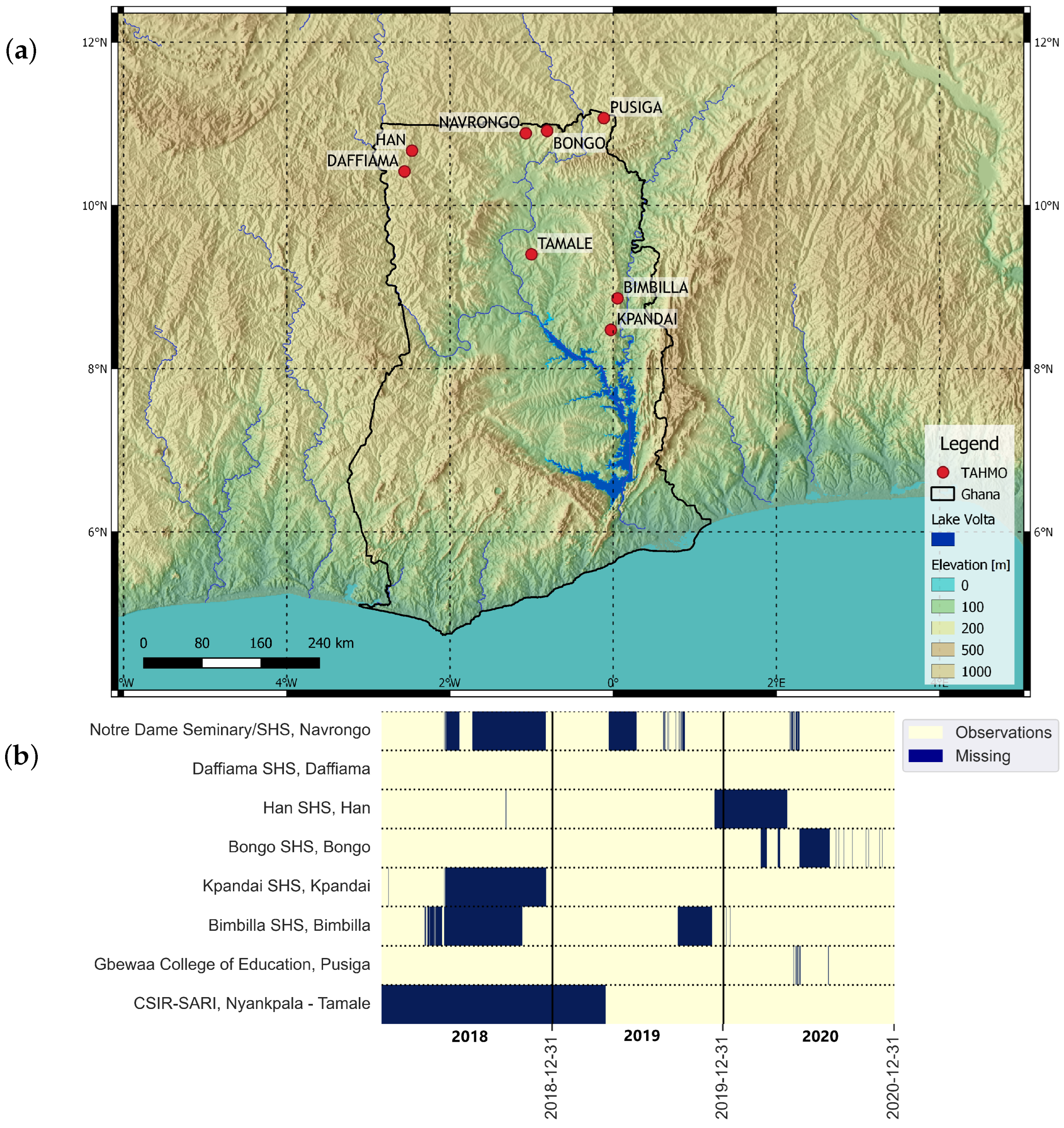
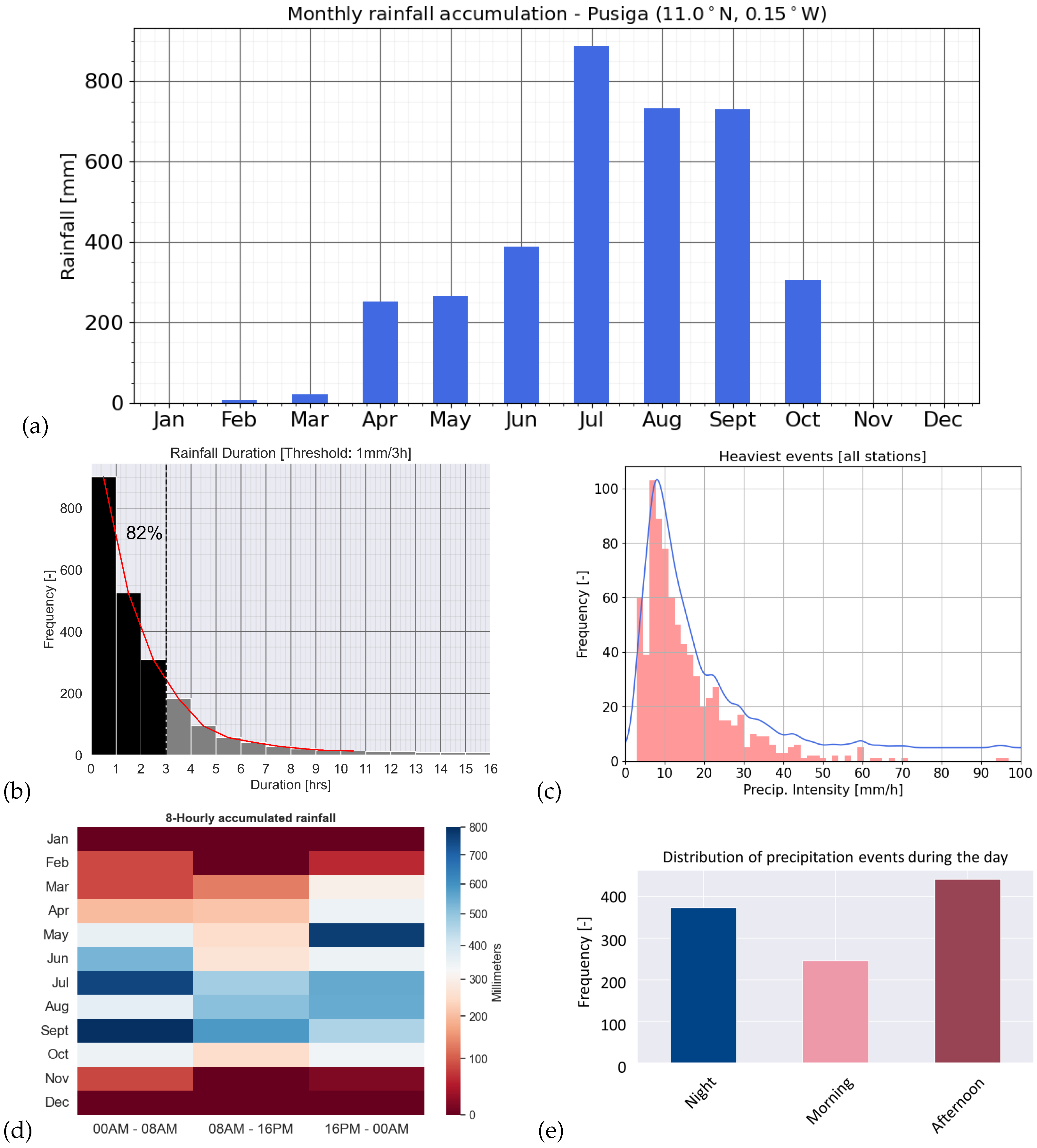
2.2. Study Area: North of Ghana

The study area is northern Ghana, between 8° N and 11° N latitude and 3° W and 0°30’ E longitude. The climate in this region corresponds to that of the broader Sudanian savanna agro-ecological zone of West Africa [25]. West Africa has one of the most extreme climatic gradients in the world, where the most significant climatic element is rainfall. The mean annual rainfall steadily increases southward towards the equator, with extremes ranging from near-zero in the arid part of the Sahel up to over 2000 mm/year in the coastal zones [26].
Northern Ghana has a unimodal rainfall regime, with a peak generally occurring during the months of July and August. The dry season in this region starts in November and lasts until late March. During this period of time, there are virtually no significant precipitation events [27]. Rainfall patterns in this area are highly regional and present a strong diurnal cycle. The main characteristics of the rainfall regime in the region of interest are visualized in Figure 3. Precipitation displays characteristics of a convective and very heavy rainfall regime: seasonal heavy short-lived thunderstorms (Figure 3b,c), short-lived events, with the majority (82%) not lasting more than 3 h, and a close to 20 mm/h median value of the heaviest rainfall events.
Figure 3d shows a progressively erratic diurnal cycle of convection during the rainy season starting from May due to the strengthening of the African Easterly Jet. A stronger African Easterly Jet consequently enhances horizontal moisture transport (visible in WV 7.3 µm data) and the formation of large mesoscale convective systems that propagate overnight and result in large accumulated rainfall values. This pattern peaks in early September where almost 1000 mm falls during nighttime. Morning hours (6 a.m.–12 p.m.) have generally the least rainfall accumulation, as well as fewer precipitation events (Figure 3e). Stable atmospheric conditions are more often found around this time of the day.
On average, northern Ghana is more often under the influence of the hot and arid North Easterly trade wind, which blows air that comes from the Sahara desert, usually carrying a considerable amount of dust, while the southern part of the country receives more maritime influx through moist SW winds.

2.3. Data Preprocessing

Sparse ground training data pose a challenge to any ML-based rainfall retrieval model. The methodology described in this section presents a way to overcome the lack of dense ground data by using an image to point approach such as described in [11]. For this purpose, TIR and WV images were cropped to create a matrix of 32 × 32 pixels (96 × 96 km) with the TAHMO station located in a central 2 × 2 pixels square. The spatial resolution of the model corresponds to the pixel size, which is approximately 3.1 km [11]. Cropped images were then grouped to form 3 h (12-image) sequences. The chosen temporal resolution is in line with the rainfall duration pattern of this area. Integrity of the sequences was mandatory: if any sequence included missing data, it was discarded from the process.
Hourly TAHMO ground measurements were accumulated into 3 h intervals to match the temporal scale of the input sequences. A threshold of 1 mm/3 h was selected to discriminate between rain and no-rain sequences. We based our choice of threshold on the short and intense nature of rainfall events in our study region, with most events lasting no more than 3 h. It is recognized that there are different possible and reasonable definitions, but 1 mm/3 h was also used in our previous work developing the first version of this model, making a direct comparison more consistent [11]. We aggregated 30-min resolution IMERG data in a similar fashion for comparison.
To include temporal information about the satellite observations, we mapped the MSG data timestamp onto a circle to represent its cyclical nature. Particularly, from the timestamp, we extracted the month number, from 0 to 11, and hour of the day, from 0 to 21, due to the sequences being 3 h in length. We performed the mapping by converting these two variables into two two-dimensional arrays using sine and cosine transformations. In this way we avoided jump discontinuities from 11 pm to midnight and December to January. Equations (1) and (2) provide the timestamp encoding, where X is the time variable in question.
X s i n = s i n ( 2 π × X m a x ( X ) )
X c o s = c o s ( 2 π × X m a x ( X ) )
The development dataset is highly skewed, as is the rainfall binary classification problem. This means that the number of no-rain sequences is much larger than rain sequences. To deal with this imbalance, we followed the methodology of [11] and used a hybrid approach of data resampling and weighted loss function.
The dataset was split in such a way that the rain sequences in the training dataset were oversampled with a ratio of 4:1 dry/rain, while both validation and test datasets had a ratio of 28.2:1 dry/rain, representative of the full 2020 data. The training dataset contained sequences from 2018, 2019, and 2020, while the validation and test datasets only had sequences from 2020. The dataset distribution was based on the minority class, i.e., rain samples, divided following an approximate 70–15–15 (training–validation–test) ratio. The dry samples were selected randomly using the corresponding dry/rain ratios (Table 1).

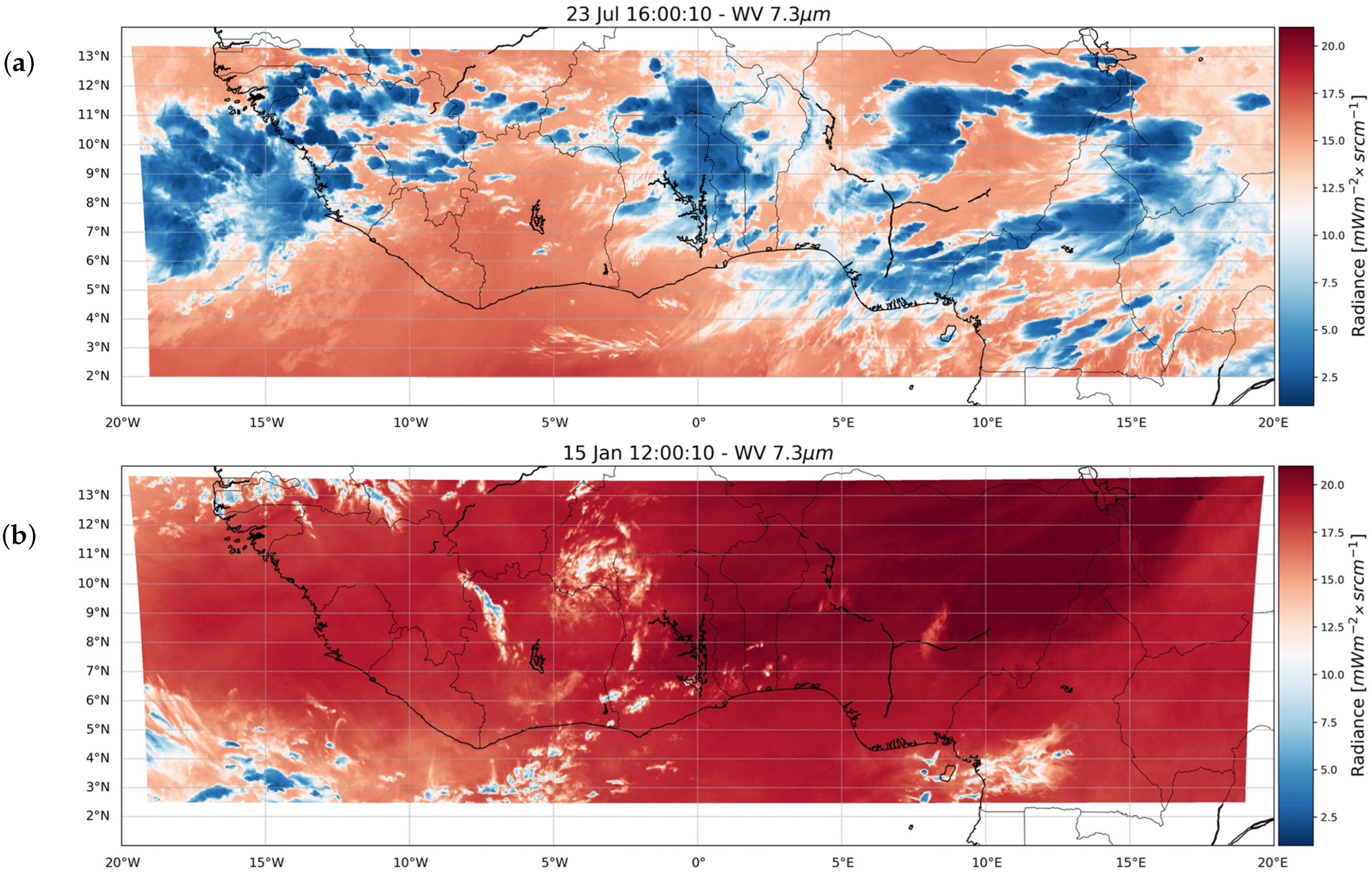
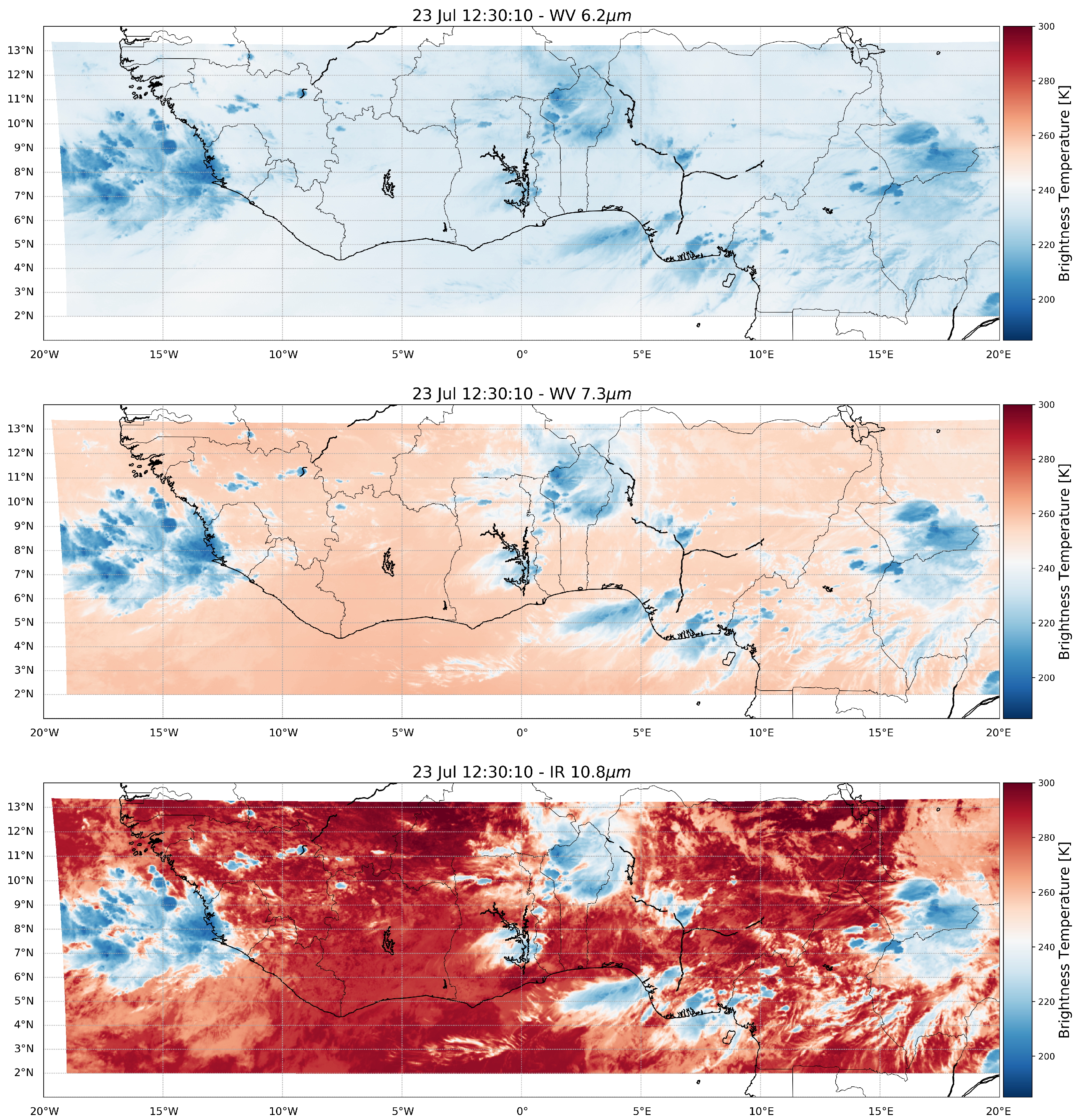
2.4. Satellite Data Analysis

To study the differences between the TIR and WV spectral channels of SEVIRI and their complementarity, satellite data were analyzed using pixel analysis. We followed a top-down approach comparing data from the two channels from the larger synoptic scale over the entirety of West Africa—20° W to 20° E—to the smaller scale (mesoscale) using already cropped MSG images from relevant sequences used for model validation.
The aim of the larger-scale comparison was to visualize the water vapor exclusion of low-level nonconvective features hidden by the West African monsoon during the rainy season. For each SEVIRI TIR channel, the relationship between observed radiance R and the equivalent brightness temperature T b is given by EUMETSAT and expressed in Equation (4). In this relation, R is the observed radiances in mW m 2 sr 1 (cm 1 ) 1 , T b is the equivalent brightness temperature in K, ν c is a central wavenumber of the spectral channel in cm 1 , c 1 and c 2 are constants with values c 1 = 2 h c 2 , c 2 = h c κ , where h is Planck’s constant, c is the speed of light, and κ is the Boltzmann constant. The central wavenumber ν and the so-called band c correction coefficients A and B were determined by EUMETSAT from a nonlinear regression of a precalculated lookup table using the Planck function for the different thermal infrared SEVIRI channels and are provided on EUMETSAT’s website [28].
T b = [ c 2 v c l o g ( 1 + c 1 v c 3 / R ) B ] / A
We analyzed sequences at the smaller scale using gray-level histograms of the normalized pixel values, positively related to equivalent brightness temperature. Because temperature is not constant with height, if the atmosphere is conditionally unstable, there is a negative temperature lapse rate Γ between the Earth surface and a layer at h e i g h t = Z that can be simplified using the relation expressed in Equation (4), where T is the absolute temperature and z the altitude.
Γ = d T d z
In raw satellite imagery, pixel radiances with values approaching the unity are bright pixels, and they translate into absorption at lower levels of the atmosphere, i.e., the effective layer is located at low levels, which corresponds to higher temperatures. Darker pixels have values closer to 0, which indicate colder temperatures of the effective layer, and therefore, its location will be at a higher altitude. Meaningful events for evaluation were selected manually based on (1) the misclassified probabilistic output values of the models, so that events for which one or both models misclassified a sequence but the combination of both corrected the classification were selected, and (2) the WV mean pixel value being at least a standard deviation away from TIR mean value.

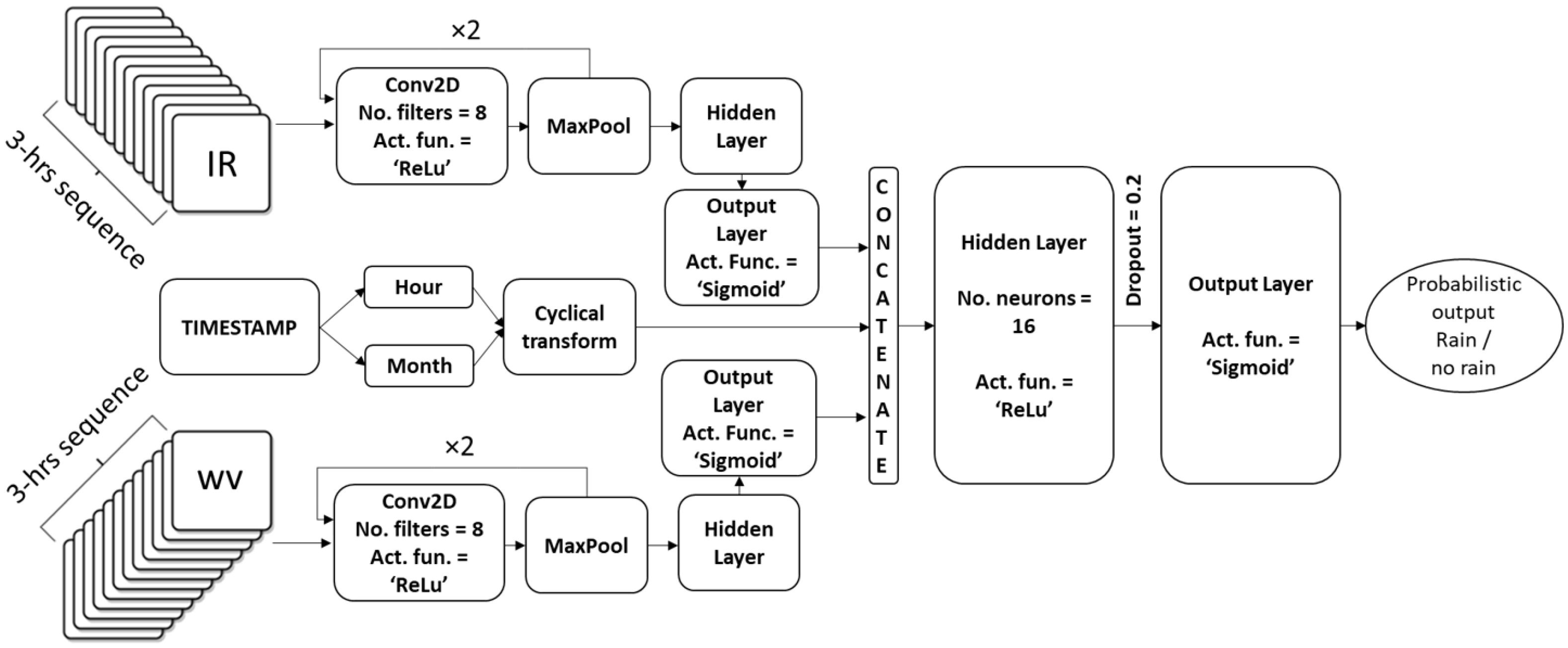
2.5. Model Development

We built our model on RainRunner [11]. We expanded the input layer to feed two different streams of twelve 32 × 32 × 1 matrices for a total of 24 input images, with one stream per each SEVIRI channel (TIR and WV).
We increased the number of nodes from 8 to 16, following the increase in the number of input images (from 12 to 24). Figure 4 illustrates a condensed diagram of the bispectral model structure. The inputs of WV and TIR are convoluted separately in order to learn information individually from each channel. The output of the convolution and pooling layers is a 2-dimensional (8 × 8 × 1) single tensor generated from each image of the sequence, i.e., 2 convolutions are applied in series. The tensors are then flattened and concatenated before being fed to a multilayer perceptron. The timestamp (month and time of the day) is added directly into the fully connected layer after preprocessing along with the 2D tensors from the convolutional layers. The model has 11,019,197 learnable parameters. The batch size was set to 64 and the learning rate was fixed to 0.0001. The number of passes trough the training dataset was fixed at 300 epochs with an early stopping callback set to 50 to halt the training in case the model was overfitting. The function for the dense layer(s) is a rectified linear function (ReLu), while the output layer function is a logistic function, or sigmoid, which returns a probabilistic output between 0 and 1, where 1 represents 100% rain and 0 is 100% dry. A decision boundary line at 0.5 is used for the classifier to make a distinction between the two classes. Lastly, a weighted loss function was applied to deal with the imbalanced dataset, where dry sequences have 0.2 and rain sequences 0.8 coefficients, which reflected the ratio of dry/rain sequences of the training dataset.

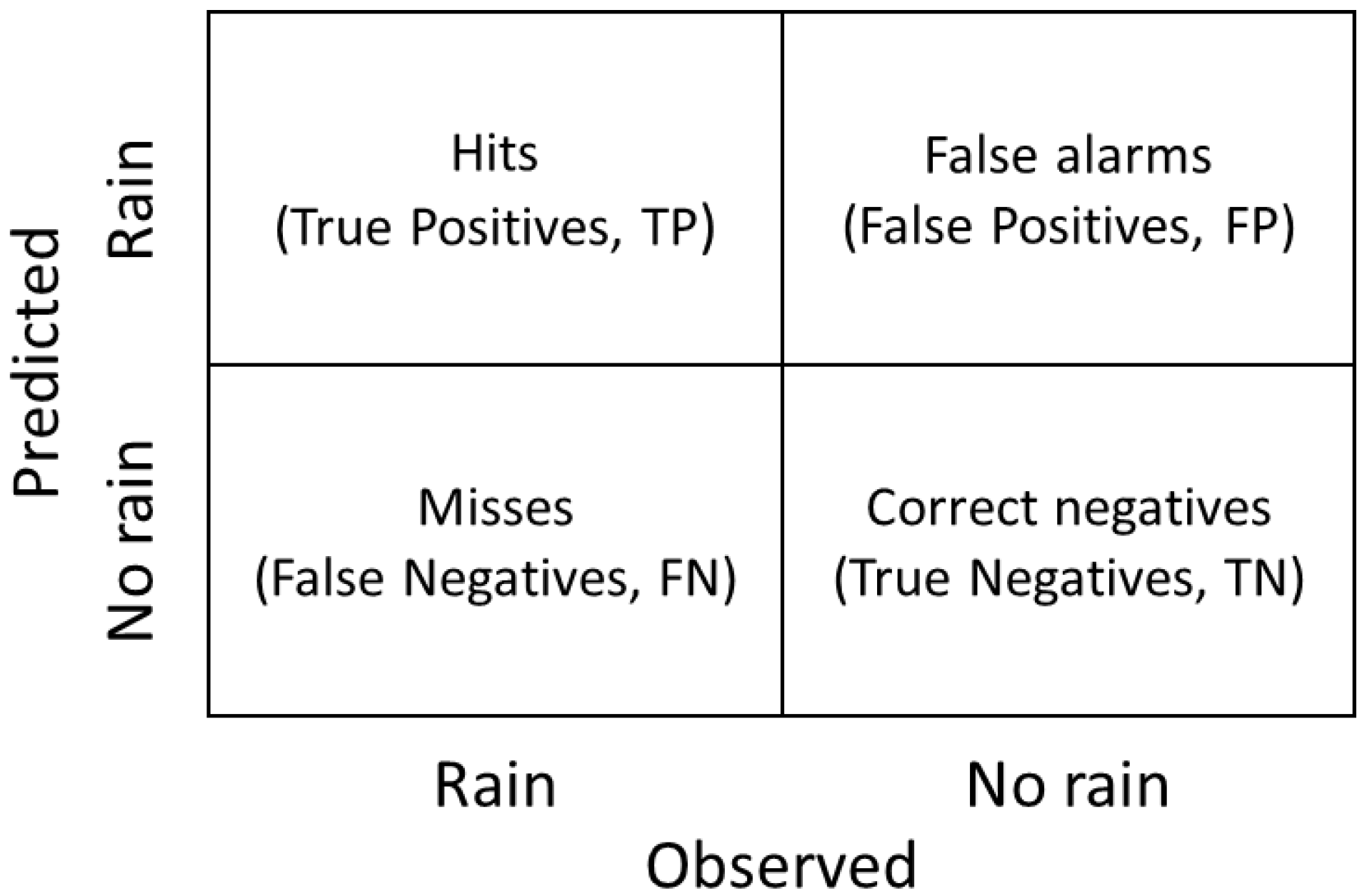
2.6. Performance Evaluation and Assessment of Data Contribution
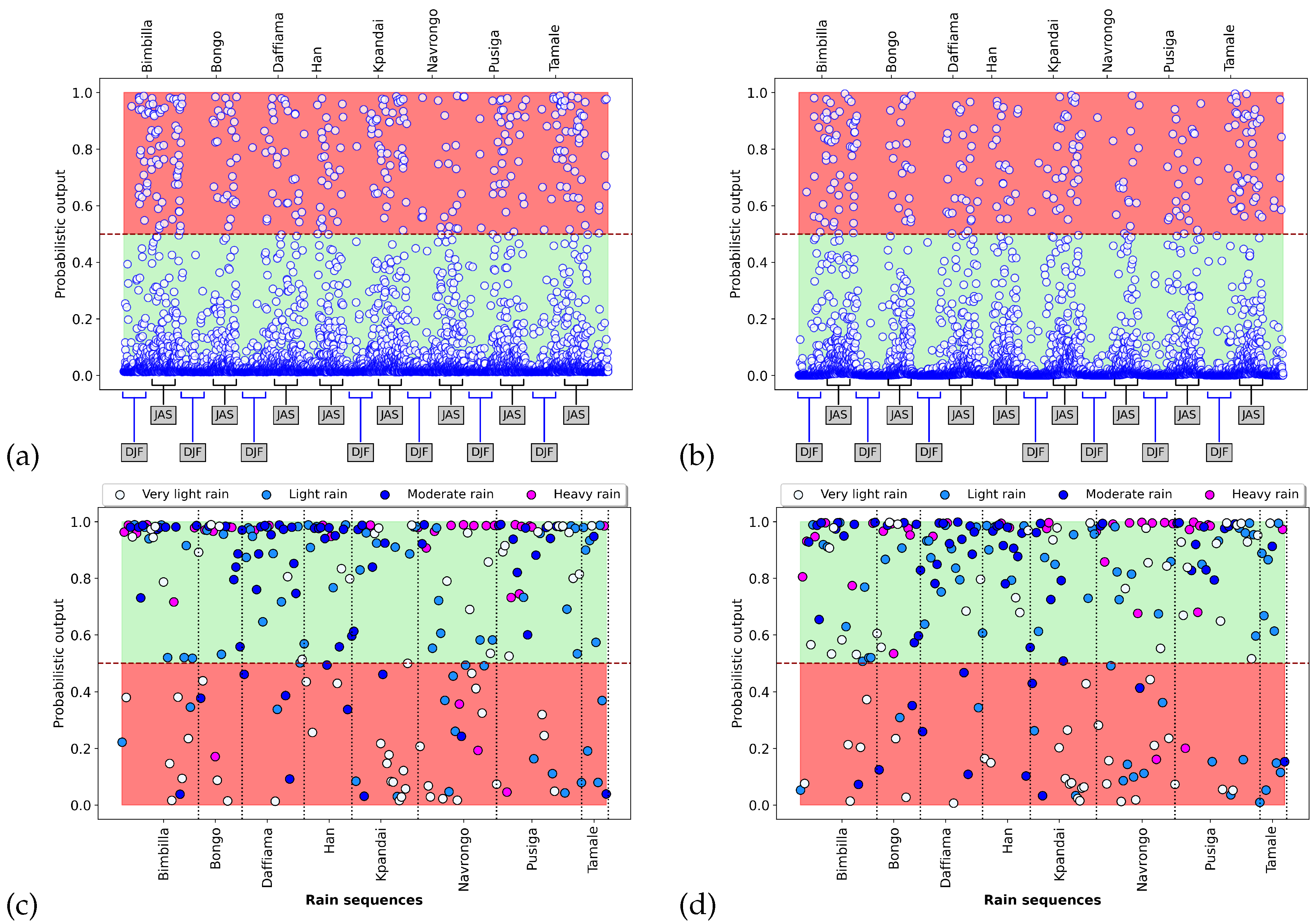
In order to assess the individual contributions of water vapor and timestamp, we conducted an ablation study in which we evaluated four models with different inputs but similar architecture/hyperparameters: (1) TIR data only; (2) WV data only; (3) TIR and WV data combined; and (4) TIR and WV data together with the observation timestamp. For a robust comparison, we applied an ensemble average to 10 runs of each model, so as to reduce the variance of the predictions. We evaluated model performance using a set of categorical metrics based on the contingency table, represented in Figure 5. These are Accuracy (Equation (5)), Probability of Detection (POD, Equation (6)), Success Ratio and its complimentary False Alarm Ratio (SR and FAR, Equation (7)), Frequency Bias (FBias, Equation (8)), F1 score (Equation (9)), and Critical Success Index (CSI, Equation (10)). POD, SR, CSI, and F1score range between 0 and 1, with 1 being the optimal value. FBias can adopt values from 0 to + , with the target value being 1. If FBias is below 1, the model is underforecasting the event; if it is above 1, it is overforecasting it. F1score represents the harmonic mean of SR and POD and is especially valuable for imbalanced problems. Hence, the best averaged models were ranked according to F1 score. Accuracy, POD, SR, FAR, FBias, and CSI are performance metrics commonly used in meteorology for dichotomous forecast verification [29,30,31]. F1 score is widely used in the Deep Learning field and is especially useful to evaluate highly skewed binary classification problems.
A c c u r a c y = T P + T N T P + F P + F N + T N
P O D = T P T P + F N
S R = 1 F A R = 1 F P T P + F P
F B i a s = P O D S R
F 1 s c o r e = 2 × S R × P O D S R + P O D
C S I = 1 1 S R + 1 P O D 1
Evaluation of model performance and of the contribution of each model input was also performed by miscassification analysis, that is, analysis of the distribution of misclassified sequences through the day and across different months, seasons, TAHMO stations, and rain intensities or categories. Rain categories were defined according to the Glossary of Meteorology of the American Meteorological Society (AMS, https://glossary.ametsoc.org/wiki/Rain (accessed on 1 June 2021)), except the “very light rain” category, which was introduced in [11] for a more detailed results analysis, and is as follows:
  • Very light rain: 1 mm/3 h < R R < 1 mm/h;
  • Light rain: 1 mm/h < R R < 2.5 mm/h;
  • Moderate rain: 2.5 mm/h < R R < 7.6 mm/h;
  • Heavy rain: R R > 7.6 mm/h.

3. Results

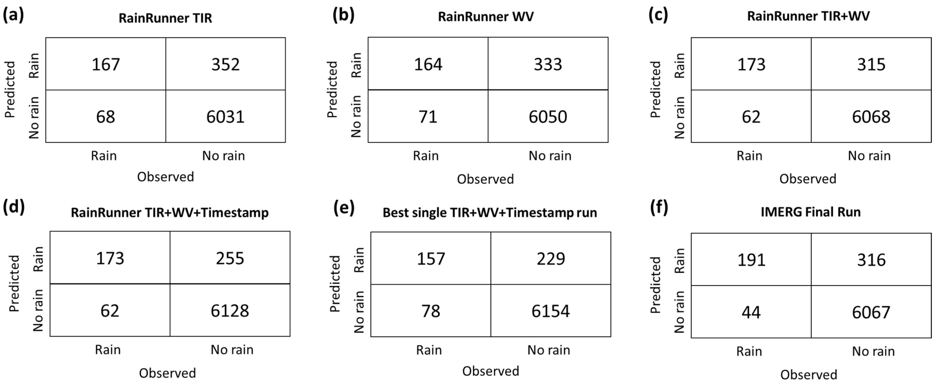
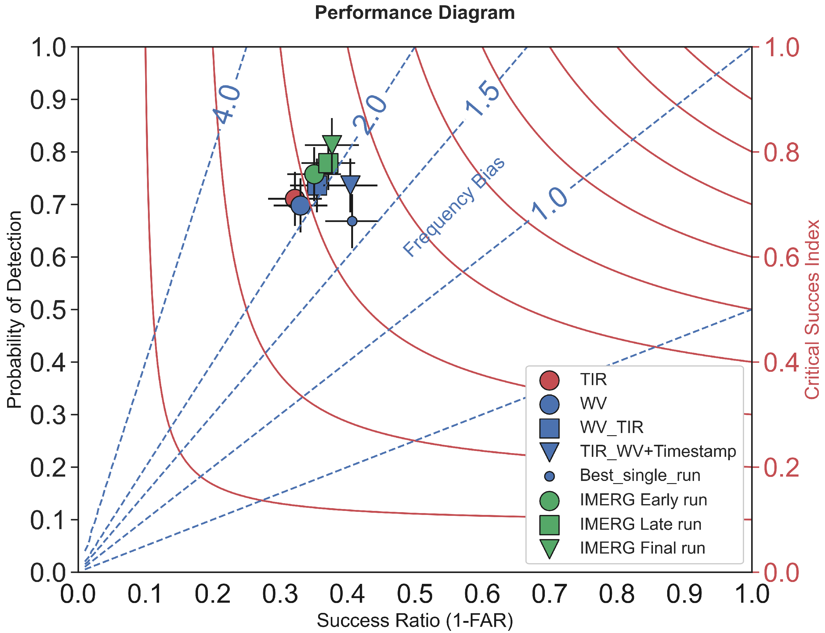
3.1. Model Performance on the Independent Test Dataset

Figure 6 displays the contingency tables of the four models evaluated here, the best single run of the model with TIR, WV, and the timestamp as input, and of IMERG Final Run for comparison. Initially, the models that use WV and TIR alone performed similarly, with the TIR model missing a slightly lower number of rain events and the WV model showing less false alarms (false positives). Combining the two channels leads to fewer misclassified dry and rainy sequences. The number of false alarms decreases further when the timestamp is included into the model. On the other hand, IMERG has considerably less misses (false negatives), which can be explained by the model making use of a constellation of LEO PMW satellites, able to sense rainfall more directly than TIR sensors. The best single run of the model with all inputs presents the overall lowest number of false alarms (229), at the expense of a high number of misses (78), which corresponds to a third of the all rainy sequences.
For better visualization, the categorical metrics are also represented in the Roebber performance diagram [29] in Figure 7, where all IMERG products are plotted as reference models. In this diagram, a perfect forecast would be in the top-right corner, with POD, SR, and CSI equal to one.
IMERG-Final has the highest number of hits (true positives). As a consequence, it also has the highest POD of all models, although it has a Fbias well above 2, which means it is severely overdetecting rainfall. The IMERG Early and Late Run products have similar Fbias, yet a lower POD and SR. IMERG Early has comparable performance to the WV_TIR model, while it is outperformed by the TIR_WV + Timestamp which achieves lower Fbias at the same short latency time. The benefit of adding WV and timestamp is noticeable in this diagram, as it progressively leads to a higher success ratio (SR) as well as a lower Fbias, reaching the lowest FBias of all models ( 1.5 < F b i a s < 2.0 ).

3.2. Misclassification Analysis

Figure 8 shows the distribution of misclassified sequences among different factors, i.e., time of the day, month, season, station, and rain category. The northernmost stations overall have fewer misclassified sequences compared with those more to the south of our study region. Overall, the combination of WV and TIR with the timestamp results in the least number of misclassifications of our developed models. The addition of the timestamp is particularly valuable during the dry season. The rainy season (boreal summer) shows a poorer performance than the dry season for all models. It is worth mentioning that IMERG has the highest number of incorrectly classified sequences during the second half of the rainy season (from July to October), highlighting the fact that the influence of the African Easterly Jet on rainfall patterns is a true challenge, even for the most advanced models. The WV model, whose strongest advantage is the correct depiction of convective motions, shows the most misclassifications for light and very light (stratiform) rain detection.
Figure 9 illustrates the contribution of the WV and the timestamp information in the model by comparing the probabilistic output of the combined model + timestamp with RainRunner TIR-only (10.8 µm). The addition of the number of the month makes the predictions for the trimester December–January–February (DJF) much lower, with values close to 0. Concretely, while the mean probabilistic output of the model using TIR alone was 0.14, it decreased to 0.005 when incorporating the timestamp. On the other hand, dry intervals during July–August–September (JAS) are still the most difficult to classify for both models. Results suggest that the addition of the time of the day is especially beneficial during the early rainy season, when the African Easterly Jet is not yet offsetting the diurnal convective cycle and rainfall is still occurring during late afternoon hours.
Figure 9c,d shows how TIR-only predictions of rainy sequences are closer to unity than the model combined with timestamp. This is particularly true for some rain events that occurred during the shoulder season (March/April or October/November) and obtained a lower probabilistic output with the model using timestamp.
Four heavy rainfall events were misclassified by the model using TIR alone, while only two heavy events were misclassified by the combined model. This is probably due to the ability of WV data to capture strong convective motions associated to heavy rainfall.

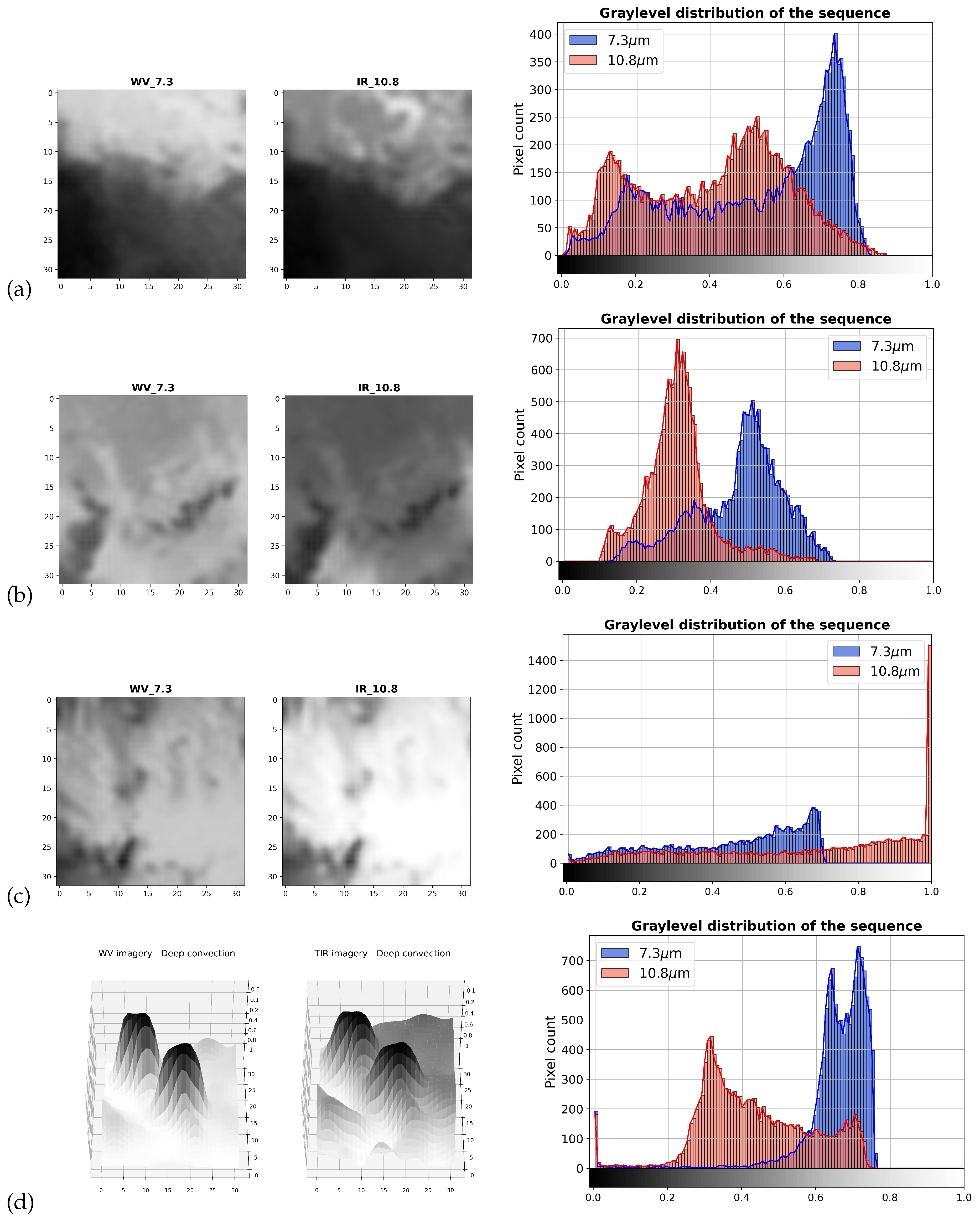
3.3. Pixel Analysis Comparison

Satellite images over large areas are useful to understand the differences between the TIR and the two WV channels. Figure 10 shows a snapshot of West African atmospheric dynamics on 23 July 2020 at noon using equivalent temperature brightness units. Midday is the time at which the solar heating cycle is at its peak and early convection is visible. The image retrieved at 10.8 µm shows information not always related to rainfall, such as many low-level clouds spread across the whole region. Where the sky is clear, the brightness temperature is an indicator of the land surface temperature (the dark red area on the upper part of the figure is near the Sahara Desert). Areas of intense convection (dark blue) are highlighted in water vapor imagery. The softer red shade shown in 7.3 µm is clearly the top of the West African Monsoon layer that acts as threshold level for this channel, hiding low-level clouds. Above this level, the African Easterly Jet transports moisture eastwards and promotes slanted convection. The largest sensitivity range for channel 5 ( 6.2 µm) is around 350 hPa, which makes this channel completely blind to the West African Monsoon as well as to most of its associated lower-level features. It is still a useful channel to locate deep convective motions that take place in the upper troposphere, where the average temperature is around 240 K.
Figure 11 displays some of the analyzed misclassified sequences where the bispectral approach proved to be useful for the model and reflected some insight into atmospheric dynamics. The output of the four evaluated models for these sequences is presented together with the corresponding ground truth in Table 2. In Figure 11, the images on the left side were selected from entire sequences for being illustrative of the atmospheric event at hand. On the right hand side, the gray-level histogram shows the pixel distribution of each corresponding sequence.
From top to bottom, Figure 11a shows a clear dry intrusion. Dry intrusions happen when a tropical system advects air from a dry source, generally right after a precipitation event. They are visible as a sharp gradient in WV imagery but are difficult to locate in TIR imagery, because warmer clouds linger for a longer period of time.
A dry slot is seen in Figure 11b. Dry slots can be a consequence of dry intrusions, or they might happen along the transition zone between convective and stratiform rain in larger mesoscale convective systems.
In these two cases, while the model using TIR data alone misclassified the sequence as rainy, the addition of WV allowed to correct it.
Figure 11c is a dry sequence from January 2020 (dry season) that was misclassified by WV as rainy. However, TIR data show that there were no rain-bearing clouds at that moment. This can happen when an anomalous low-level moist southerly circulation peaks up during certain days of the dry season, while, at higher levels, dry air is present. In this situation, the 7.3 µm channel retrieves water vapor content from lower levels resulting in incorrect predictions.
Figure 11d is a 3D surface plot of the 2D TIR and WV data, aimed at better showing convective motions of a violent rain event as seen from both channels. The Z-axis corresponds to the pixel values. The gray-level of each pixel in WV imagery gives information about the layer depth and clearly shows where strong convection occurs.
As for the gray-level histograms, two distinct peaks are observable in each histogram. That is, the two channels generate an asymmetric bimodal pixel distribution at different brightness temperatures. In the case of WV imagery, the peak is an indication of the most frequently occurring height of the effective layer during the sequence.

4. Discussion

This study proposed a Deep Learning approach to tackle the challenge of rainfall detection in the Sudanian savanna of West Africa by using bispectral MSG data, i.e., TIR and WV data, as well as temporal information. WV data proved to be useful in detecting the midlevel African Easterly Jet, a main driver of rainfall dynamics in this area. This jet creates a thermodynamic environment favorable for deep convection, observed in WV data without the contamination from low-level clouds observed in TIR data. Furthermore, results show the complementarity of the two MSG channels in scenarios where a monospectral approach would result in misclassifications (Table 2). WV allows to reduce the number of false alarms and increase the success ratio in cases where dry air masses—dry slots and dry intrusions—in between tropical systems, missed in TIR data, suppress rainfall (Figure 11a,b and Appendix A). While TIR data alone would detect the rain-bearing clouds and misclassify these events as rain, the addition of WV data allows to correct the classification. Another scenario in which WV and TIR results are complementary for correct rainfall binary classification is when there is low-level moisture with no rain-bearing clouds. Although WV data alone would misclassify these cases as rain, TIR data are able to correct them for the absence of rain-bearing clouds. For certain events that are more difficult to identify, the gray-level histogram can be helpful to distinguish dry from wet conditions during dry intrusions and dry slots, indicated by the the distance between the mode of the WV and TIR pixel distributions. Of the three scenarios—dry intrusions, dry slots, and low-level moisture—dry intrusions are the most challenging because of the sharp gradient present in the image (Figure 11a). This sharp gradient can lead to TIR data alone misclassifying rainfall with high certainty, making it difficult for the bispectral model to capture the correct development of the dry air advection into the rainfall area.
Incorporating temporal information further allows the model to learn regional seasonal and diurnal rainfall patterns. Its contribution is most evident during the dry season, when the model correctly expects mostly dry sequences. This is most advantageous in scenarios with low-level moisture during the dry season, when adding timestamp information reduces rainfall misclassification (Figure 11c and Appendix A). In fact, the misclassification analysis shows that the model based only on WV data achieves the lowest performance among all models during the dry season. This is because of the variable height of the effective layer. During the dry season, there is very dry air higher up in the atmosphere, and the satellite sensor might detect some anomalous low-level moist currents that are not correlated with rainfall and that might be misclassified as rain. However, these misclassifications can be corrected with the addition of TIR and temporal information. Because most of the analyzed dry slots and dry intrusions events (tables in the Appendix A) take place during the early or late rainy season, when the atmosphere is more dynamic, the timestamp contribution is unclear. In this scenario, adding timestamp information reduced the chances of misclassification in 50% of the analyzed cases.
The flipside of including WV data is that it fails to retrieve stratiform rainfall. Stratiform or warm rain is the precipitation that falls from low-level clouds and is usually associated with light rainfall events. However, its relationship with low-level clouds remains very uncertain, since the presence of such clouds is only sporadically linked to rainfall [32]. The model using WV alone is the worst performing model for very light and light rain (Figure 8), likely to be found in stratiform clouds. Depending on the application, this insensitivity to low-level clouds might be a strength or a weakness. More than 80% of the rainfall in tropical inland areas comes from mesoscale convective systems (MCs), and in fact, the presence of low clouds or high clouds such as thin-iced cirrus leads to an overforecast of precipitation in models that only make use of TIR data, which can be seen in Figure 6 and Figure 7, Table 2, and the Annex. The adoption of Channel 5 (WV 6.2 µm as opposed to the used 7.3 µm) would focus the model even more on deep convective events that are strictly related to heavy rainfall events, since it only detects upper-level WV structures (Figure 10). However, no information on stratiform rain and shallow convection can be extracted from this channel, so it would result in more missed events. Looking at the Roebber diagram in Figure 7, a main drawback of our approach is the low POD, which might be partly explained by our model missing these kinds of light rainfall events.
Along the same line, the discrepancy in misclassified sequences between northern and more southern stations (Figure 8) is in agreement with the literature, and it is most likely due to a progressively higher availability of moisture towards the coast, which leads to a slight increase in rain from warm clouds [33].
Our approach can provide the basis to develop a full alternative solution to the established Cold Cloud Duration (CCD) method. This method is a cloud indexing statistical approach applied to the TIR channel to distinguish convective rain clouds from nonrain low clouds. It assumes a positive linear relationship between cloud tops and rainfall to find an optimal temperature threshold for a certain area [34]. However, because of the complexities of convective rainfall, both the temperature threshold and the linear regression relationship depend on local characteristics of the area under consideration. Even if the region of interest is divided into many calibration subareas, the results exhibit several discontinuities in the rainfall estimates. Additionally, each calibration area requires many ground measurements. At the moment, West African gauge coverage is far from sufficient to make this method a reliable option. The strength of this method relies on its simple approach to achieve reliable results at very low temporal resolutions (POD: 0.69, SR: 0.75, BIAS: 0.9 for wet dekadals detection) [6]. The combination of the TIR and WV channels automatically excludes nonconvective features within the whole region of interest. Furthermore, the temporal resolution is higher than for TAMSAT (3hrs vs daily), which is very beneficial in a convective precipitation context. Similarly to the CCD-based CHIRPS and TAMSAT, the model developed in this study is specifically designed for equatorial Africa. The addition of WV data is expected to be less effective in detecting rainfall outside the tropics, where convective rainfall is less dominant. Different factors play a role in rainfall formation in midlatitudes, in particular frontal systems.
Finally, an important advantage of the model is the short latency time of 3 h, as compared with the 3.5 months latency of IMERG Final Run and the 12 h latency of IMERG Late Run. Only IMERG Early Run has a comparable latency time, i.e., 4 h. Precipitation estimates have an important operational value and are essential for crop models and applications such as flood and drought monitoring—for which timeliness is essential in an operational setting.
A promising direction for further development is to transform binary rainfall detection into rainfall estimation. However, geostationary (GEO) IR images have the limitation of providing only indirect rainfall estimates. Passive Microwave Sensors (PMWs) remain the most direct satellite observations for rainfall retrieval, capable of retrieving the rainfall rate by receiving the backscattered signal of hydrometeors. Therefore, the addition of PMW estimates could prove beneficial. As a starting point, rainfall estimates derived from GEO IR imagery could be locally adjusted whenever a PMW observation is available for that region, although post-processing calibration is required to account for grid mismatch [35]. Another advised future development is to increase the temporal and spatial resolution of the model. Certain rainfall events are so highly localized in space and time that the current scale (i.e., 3 h 96 km × 96 km sequences) is too coarse for their detection. As an example, the heavy rain event in Pusiga in May (Figure A1) was incorrectly classified by all models including IMERG Final Run. A well-defined small dark blob in WV imagery appears only at the end of the sequence, while the previous images contained mostly bright pixels that made the sequence easily misclassified as dry. Moreover, a higher temporal resolution would lead to fewer incomplete sequences, which would increase the size of the development dataset. Because most rainfall in this area is attributed to localized pockets of rapid moist air ascent, which are sometimes not larger than a few kilometers, reducing the area of the cropped MSG images could also be beneficial for their detection. On this matter, the new Meteosat Third Generation, for which the first satellite was launched in December 2022, is set to deliver higher spatial (2 km) and temporal (10 min) resolution [4]. These new data could potentially allow the WV channel to detect smaller-scale rising air motions even with the current input shape.
The combination of multiple SEVIRI channels to enhance low-level features by applying a temperature brightness difference between relevant channels might improve the detection of warm rainfall. However, it is likely that precipitation will be more overdetected unless a better relation between the two variables is defined through a T b R R relationship. On the other hand, the adoption of the other WV channel 6.2 µm may bring more reliable results on the detection of heavy rainfall events, which account for most of the accumulated rainfall on the ground.

5. Conclusions

This work shows that a DL model is able to tackle rainfall detection in regions where sparse rain gauge networks and erratic precipitation patterns pose a challenge to existing rainfall estimation methods. The incorporation of water vapor information into the model is noticeable and results in a reduced number of false alarms. The true value of WV data for rainfall detection lies in its capacity to detect dry air intrusions into tropical easterly waves, which is of particular interest for regions close to the Sahara Desert. We also show how dry intrusions and dry slots result in false positives using only TIR data, which might be the reason why TIR rainfall products tend to overdetect rainfall. This can be corrected with the addition of WV data. However, using WV data alone can also result in false positives in scenarios with low-level moisture that occur most often during the dry season and that can be corrected by TIR data. This points to the complementarity of WV and TIR data for satellite rainfall estimation in Southern West Africa. Another new input to the model from the original TIR-only version [11] is the temporal information related to date and time. Results reveal that while the addition of temporal information is beneficial in scenarios with anomalous low-level moisture during the dry season, it does not have a clear effect during the rainy season. Finally, our approach allows to decrease false alarms and reach a lower FBias than the much more complex state-of-the-art IMERG Final Run (FBias < 2.0).

Author Contributions

Conceptualization, M.E.-C., F.C., R.T., M.-C.t.V. and N.v.d.G.; methodology, M.E.-C., F.C. and R.T.; software, M.E.-C., F.C. and R.T.; validation, F.C.; formal analysis, F.C., M.E.-C., R.T. and M.-C.t.V.; investigation, F.C.; resources, M.E.-C.; data curation, M.E.-C.; writing—original draft preparation, F.C.; writing—review and editing, F.C., M.E.-C., R.T., M.-C.t.V. and N.v.d.G.; visualization, F.C. and M.E.-C.; supervision, M.E.-C., R.T., M.-C.t.V. and N.v.d.G. All authors have read and agreed to the published version of the manuscript.

Funding

This research was partially funded by the European Commission under ’TEMBO Africa’ grant number 101086209.

Institutional Review Board Statement

Not applicable.

Informed Consent Statement

Not applicable.

Data Availability Statement

TAHMO data can be accessed on the TAHMO Data Portal (https://portal.tahmo.org, accessed on 1 September 2021). Only data from demo stations and limited datasets can be requested without configuring an account. For access to all data, a data request form must be submitted. IMERG data are available in different forms on the Precipitation Data Directory of the Global Precipitation Measurement (https://gpm.nasa.gov/data/directory, accessed on 1 September 2021). Data used in this study were downloaded from the GES DISC site (https://disc.gsfc.nasa.gov/datasets/GPM_3IMERGHH_06/summary?keywords=%22IMERG%20final%22, accessed on 1 September 2021). High-Rate SEVIRI Level 1.5 Image Data-MSG-0 degree data can be requested after registra- 538 tion via the Eumetsat Earth Observation Portal (https://eoportal.eumetsat.int, accessed on 1 September 2021). Finally, all code produced during this study is available upon request.

Conflicts of Interest

The authors declare no conflict of interest.

Appendix A

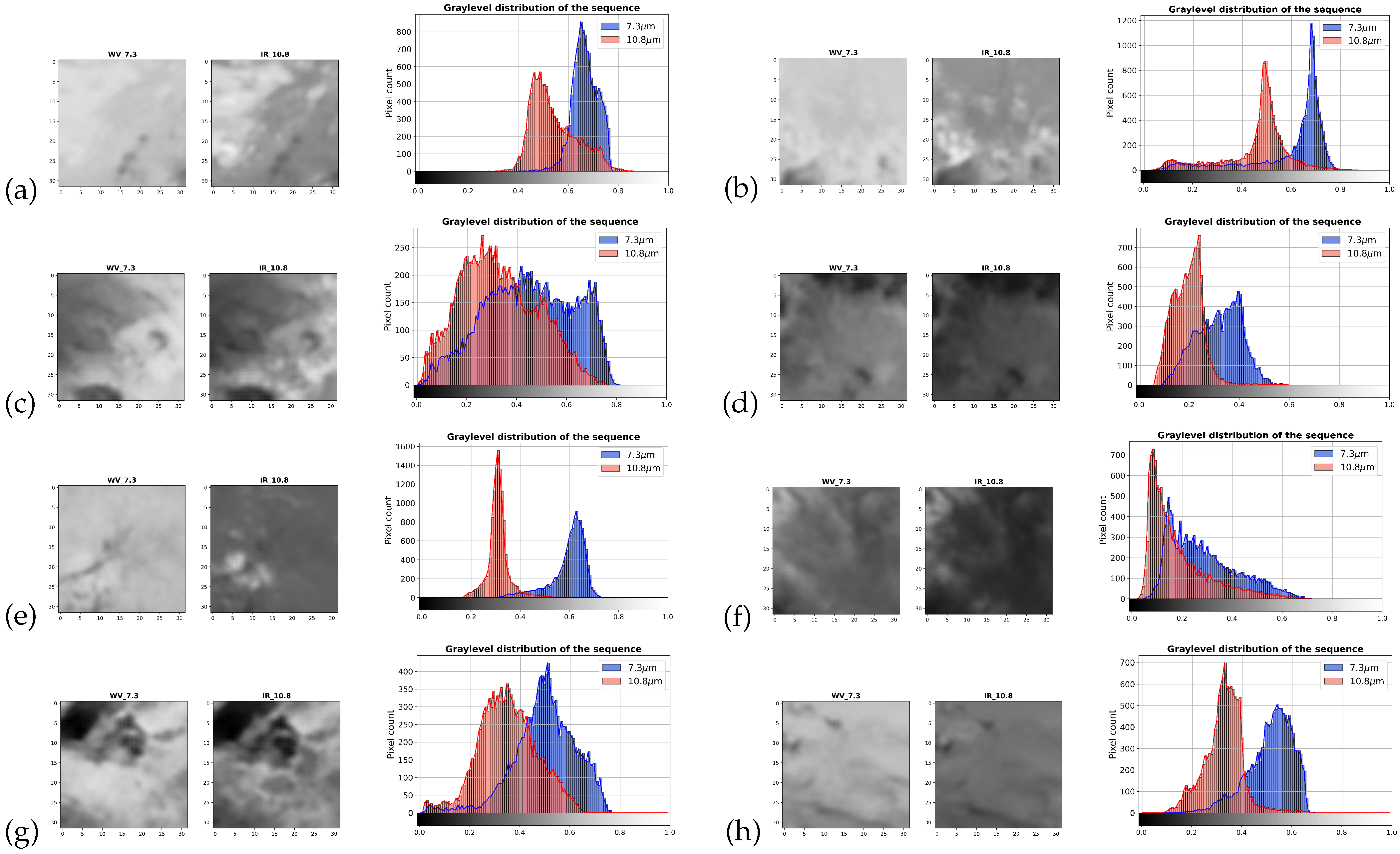
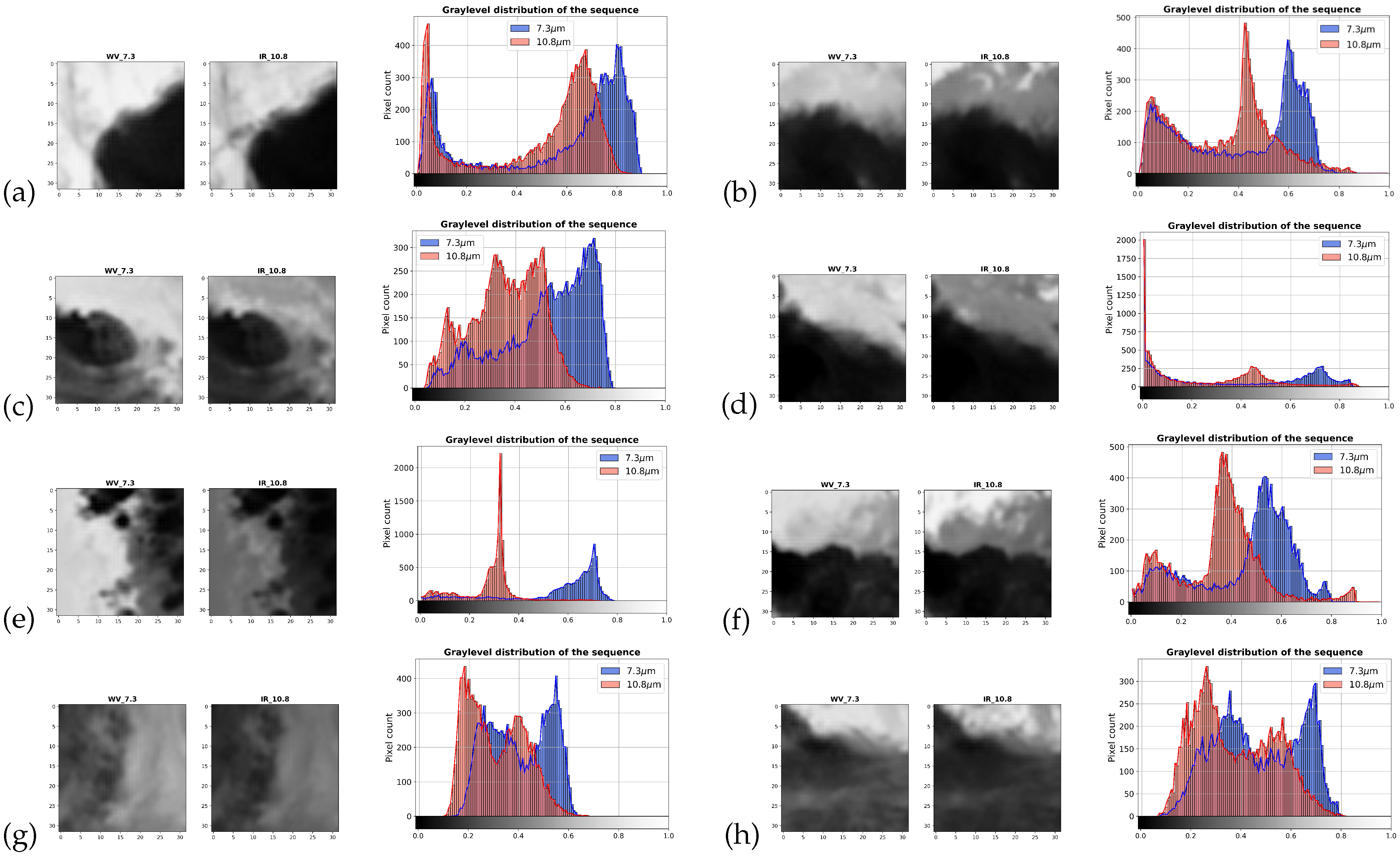
Appendix A.1. Pixel Analysis

Figure A1. Example of a misclassified rain sequence in WV imagery due to coarse temporal resolution. Pusiga—May 2020.
Atmosphere 14 00974 g0a1

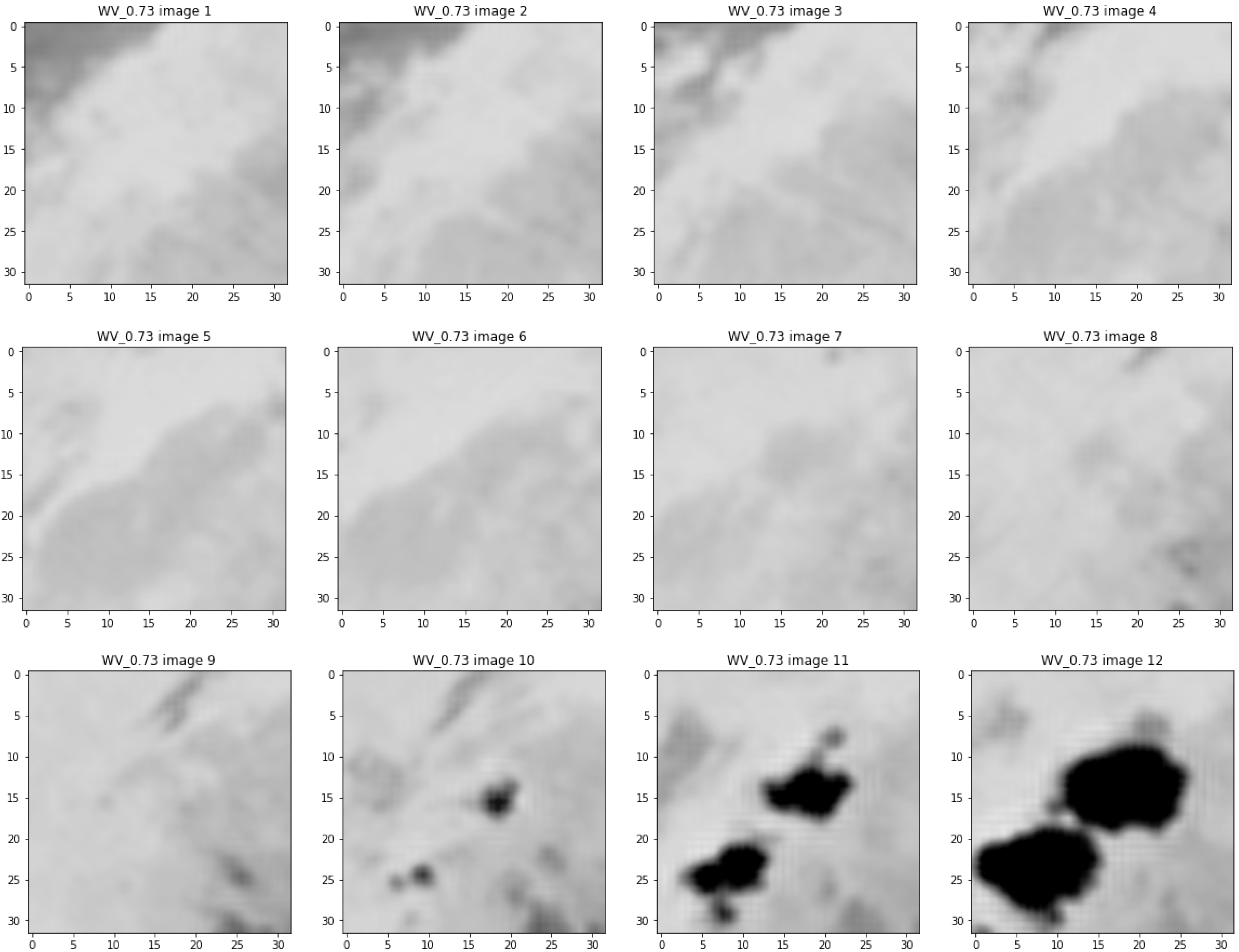
Appendix A.2. Dry Slots

Figure A2. Dry slots observed at TAHMO locations. The characteristics of each dry slot are presented in Table A1.
Atmosphere 14 00974 g0a2
Table A1. Location, date and time of the dry slots depicted in Figure A2, together with the corresponding grountruth (rain = 1/no-rain = 0) and resulting probabilistic output of the different models.
EventGround TruthTIRWVTIR + WVTIR + WV + Timestamp
(a) Bimbilla, 2020.09.07, 09 h00.510.030.0070.17
(b) Bimbilla, 2020.09.12, 06 h00.560.540.230.39
(c) Han, 2020.10.01, 15 h00.730.340.420.33
(d) Bongo, 2020.04.10, 15 h00.660.280.490.38
(e) Bongo, 2020.05.09, 12 h00.410.110.320.35
(f) Daffiama, 2020.05.15, 15 h00.740.280.470.25
(g) Tamale, 2020.06.14, 12 h00.520.090.290.23
(h) Navrongo, 2020.06.20, 15 h00.450.040.350.50

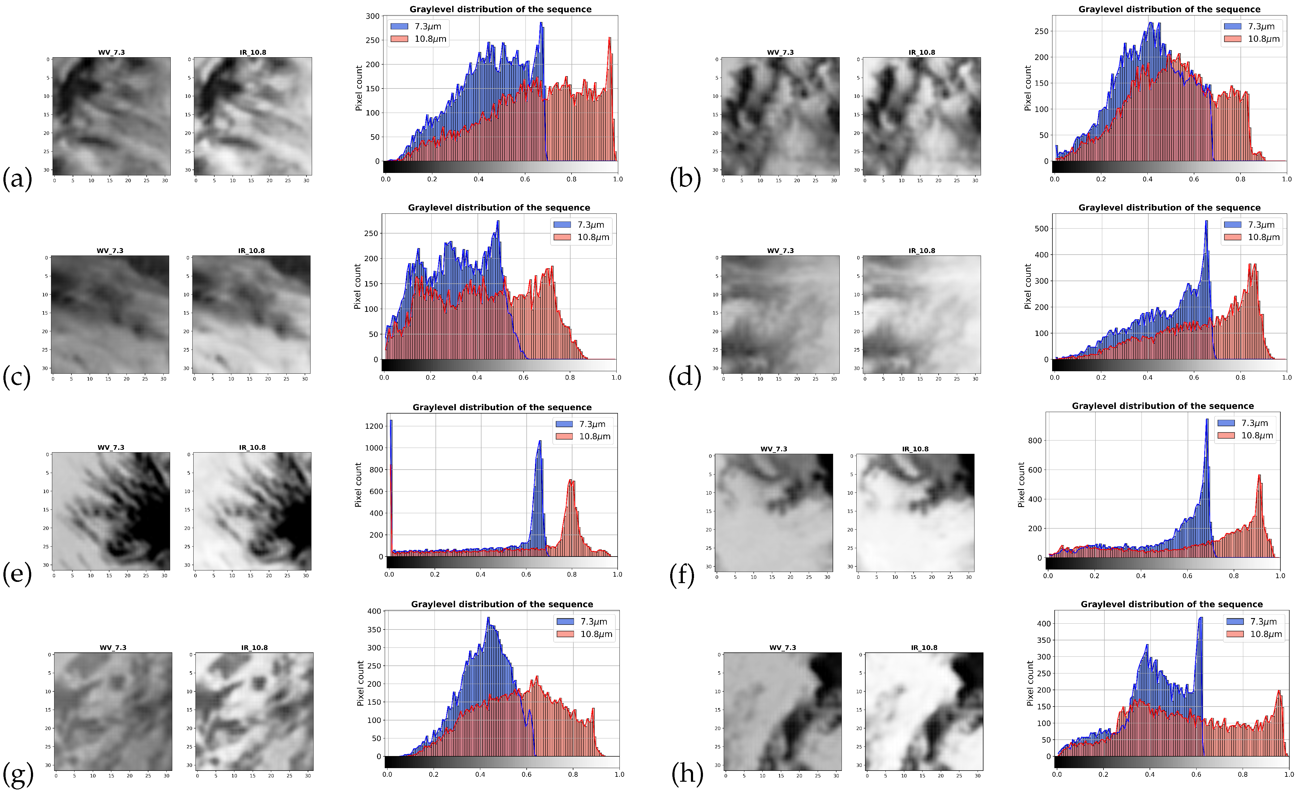
Appendix A.3. Dry Intrusions

Figure A3. Dry intrusions observed at TAHMO locations. The characteristics of each dry intrusion are presented in Table A2.
Atmosphere 14 00974 g0a3
Table A2. Location, date and time of the dry intrusions depicted in Figure A3, together with the corresponding grountruth (rain = 1/no-rain = 0) and resulting probabilistic output of the different models.
EventGround TruthTIRWVTIR + WVTIR + WV + Timestamp
(a) Bimbilla, 2020.03.22, 15 h00.570.140.670.17
(b) Bimbilla, 2020.05.06, 21 h00.920.450.640.23
(c) Bimbilla, 2020.07.26, 12 h10.510.260.750.78
(d) Bimbilla, 2020.09.30, 15 h00.770.690.460.59
(e) Navrongo, 2020.05.17, 12 h00.810.410.690.48
(f) Pusiga, 2020.05.06, 00 h00.500.340.240.29
(g) Pusiga, 2020.07.15, 03 h00.510.370.460.54
(h) Bongo, 2020.09.25, 12 h00.620.270.440.44

Appendix A.4. Low-Level Moisture

Figure A4. Low-level moisture events observed at TAHMO locations during dry season. The characteristics of each low-level moisture event are presented in Table A3.
Atmosphere 14 00974 g0a4
Table A3. Location, date and time of the low-level moisture events depicted in Figure A4, together with the corresponding grountruth (rain = 1/no-rain = 0) and resulting probabilistic output of the different models.
EventGround TruthTIRWVTIR + WVTIR + WV + Timestamp
(a) Bimbilla, 2020.02.11, 18 h00.420.830.280.30
(b) Bimbilla, 2020.12.22, 12 h00.410.650.370.18
(c) Daffiama, 2020.01.22, 21 h00.280.540.200.02
(d) Daffiama, 2020.01.23, 06 h00.220.660.14<0.01
(e) Kpandai, 2020.01.25, 00 h00.430.580.180.02
(f) Kpandai, 2020.10.21, 00 h00.300.630.370.23
(g) Navrongo, 2020.02.12, 00 h00.070.500.24<0.01
(h) Pusiga, 2020.02.11, 18 h00.080.550.240.05

References

  1. FAO. Ghana at a Glance. Available online: https://www.fao.org/ghana/fao-in-ghana/ghana-at-a-glance/en/#:~:text=Agriculture%20contributes%20to%2054%20%25%20of,food%20needs%20of%20the%20country (accessed on 1 December 2022).
  2. Bechtold, P. Convective Precipitation. Available online: https://confluence.ecmwf.int/display/FUG/9.6+Convective+Precipitation#id-9.6ConvectivePrecipitation-ConvectivePrecipitation (accessed on 1 December 2022).
  3. Coz, C.L.; van de Giesen, N. Comparison of Rainfall Products over Sub-Saharan Africa. J. Hydrometeorol. 2020, 21, 553–596. [Google Scholar] [CrossRef]
  4. ESA. Meteosat Third Generation Takes Major Step towards Its First Launch. Available online: https://www.eumetsat.int/meteosat-third-generation (accessed on 1 December 2022).
  5. Shen, C.; Chen, X.; Laloy, E. Editorial: Broadening the Use of Machine Learning in Hydrology. Front. Water 2021, 3, 681023. [Google Scholar] [CrossRef]
  6. Tarnavsky, E.; Grimes, D.; Maidment, R.; Black, E.; Allan, R.P.; Stringer, M.; Chadwick, R.; Kayitakire, F. Extension of the TAMSAT satellite-based rainfall monitoring over Africa and from 1983 to present. J. Appl. Meteorol. Climatol. 2014, 53, 2805–2822. [Google Scholar] [CrossRef] [Green Version]
  7. Funk, C.; Peterson, P.; Landsfeld, M.; Pedreros, D.; Verdin, J.; Shukla, S.; Husak, G.; Rowland, J.; Harrison, L.; Hoell, A.; et al. The climate hazards infrared precipitation with stations—A new environmental record for monitoring extremes. Sci. Data 2015, 2, 150066. [Google Scholar] [CrossRef] [Green Version]
  8. Dybkjær, G. A simple self-calibrating cold cloud duration technique applied in West Africa and Bangladesh. Geogr. Tidsskr.-Dan. J. Geogr. 2003, 103, 83–97. [Google Scholar] [CrossRef]
  9. Satgé, F.; Defrance, D.; Sultan, B.; paule Bonnet, M.; Rouche, N.; Pierron, F.; emmanuel Paturel, J.; Satgé, F.; Defrance, D.; Sultan, B.; et al. Evaluation of 23 gridded precipitation datasets across West Africa to cite this version: HAL Id: Hal-02626156. J. Hydrol. 2020, 581, 124412. [Google Scholar] [CrossRef] [Green Version]
  10. Atiah, W.A.; Amekudzi, L.K.; Aryee, J.N.A.; Preko, K.; Danuor, S.K. Validation of satellite and merged rainfall data over Ghana, West Africa. Atmosphere 2020, 11, 859. [Google Scholar] [CrossRef]
  11. Estébanez-Camarena, M.; Taormina, R.; van de Giesen, N.; ten Veldhuis, M.C. The Potential of Deep Learning for Satellite Rainfall Detection over Data-Scarce Regions, the West African Savanna. Remote Sens. 2023, 15, 1922. [Google Scholar] [CrossRef]
  12. Maranan, M.; Fink, A.H.; Knippertzand, P. Rainfall Types over Southern West Africa: Objective Identification, Climatology and Synoptic Environment. Q. J. R. Meteorol. Soc. 2018, 144, 1628–1648. [Google Scholar] [CrossRef] [Green Version]
  13. Kidd, C.; Huffman, G. Global precipitation measurement. Meteorol. Appl. 2011, 18, 334–353. [Google Scholar] [CrossRef]
  14. Aoki, P.M. CNNs for Precipitation Estimation from Geostationary Satellite Imagery; Course report: Deep Learning for Computing Vision; Standford University: Stanford, CA, USA, 2017; pp. 1–9. [Google Scholar]
  15. Moraux, A.; Dewitte, S.; Cornelis, B.; Munteanu, A. Deep learning for precipitation estimation from satellite and rain gauges measurements. Remote Sens. 2019, 11, 2463. [Google Scholar] [CrossRef] [Green Version]
  16. Barbero, G.; Moisello, U.; Todeschini, S. Evaluation of the Areal Reduction Factor in an Urban Area through Rainfall Records of Limited Length: A Case Study. J. Hydrol. Eng. 2014, 19, 05014016-1. [Google Scholar] [CrossRef]
  17. Tomassini, L.; Parker, D.; Stirling, A.; Bain, C.; Senior, C.; Milton, S. The interaction between moist diabatic processes and the atmospheric circulation in African Easterly Wave propagation: The interaction between moist processes and circulation in AEWs. Q. J. R. Meteorol. Soc. 2017, 143, 3207–3227. [Google Scholar] [CrossRef] [Green Version]
  18. Tomassini, L. The Interaction between Moist Convection and the Atmospheric Circulation in the Tropics. Bull. Am. Meteorol. Soc. 2020, 101, E1378–E1396. [Google Scholar] [CrossRef] [Green Version]
  19. Berry, G.J.; Thorncroft, C. Case Study of an Intense African Easterly Wave. Mon. Weather Rev. 2005, 133, 752–766. [Google Scholar] [CrossRef] [Green Version]
  20. ESA. MSG’s SEVIRI Instrument; ESA EUMETSAT; ESA: Paris, France, 2016; p. 33. [Google Scholar]
  21. Selami, N.; Sèze, G.; Gaetani, M.; Grandpeix, J.Y.; Flamant, C.; Cuesta, J.; Noureddine, B. Cloud Cover over the Sahara during the Summer and Associated Circulation Features. Atmosphere 2021, 12, 428. [Google Scholar] [CrossRef]
  22. van de Giesen, N.; Hut, R.; Selker, J. The Trans-African Hydro-Meteorological Observatory (TAHMO). Wiley Interdiscip. Rev. Water 2014, 1, 341–348. [Google Scholar] [CrossRef] [Green Version]
  23. Schneider, U.; Becker, A.; Finger, P.; Meyer-Christoffer, A.; Ziese, M.; Rudolf, B. GPCC’s new land surface precipitation climatology based on quality-controlled in situ data and its role in quantifying the global water cycle. Theor. Appl. Climatol. 2014, 115, 15–40. [Google Scholar] [CrossRef] [Green Version]
  24. Tan, J.; Huffman, G.J.; Bolvin, D.T.; Nelkin, E.J. IMERG V06: Changes to the Morphing Algorithm. J. Atmos. Ocean. Technol. 2019, 36, 2471–2482. [Google Scholar] [CrossRef]
  25. Windmeijer, P.; Andriesse, W. Inland Valleys in West Africa: An Agro-Ecological Characterization of Rice-Growing Environments; International Institute for Land Reclamation and Improvement: Wageningen, The Netherlands, 1993. [Google Scholar]
  26. Nicholson, S. The West African Sahel: A Review of Recent Studies on the Rainfall Regime and Its Interannual Variability. ISRN Meteorol. 2013, 2013, 453521. [Google Scholar] [CrossRef]
  27. Knippertz, P.; Fink, A.H. Dry-Season Precipitation in Tropical West Africa and Its Relation to Forcing from the Extratropics. Mon. Weather Rev. 2008, 136, 3579–3596. [Google Scholar] [CrossRef]
  28. Schmetz, J.; Pili, P.; Tjemkes, S.; Just, D.; Kerkmann, J.; Rota, S.; Ratier, A. SEVIRI Calibration. Bull. Am. Meteorol. Soc. 2002, ES52–ES53. [Google Scholar] [CrossRef]
  29. Roebber, P.J. Visualizing Multiple Measures of Forecast Quality. Weather Forecast. 2009, 24, 601–608. [Google Scholar] [CrossRef] [Green Version]
  30. Karagiannidis, A.; Lagouvardos, K.; Kotroni, V. The use of lightning data and Meteosat Infrared imagery for the nowcasting of lightning activity. Atmos. Res. 2015, 168, 57–69. [Google Scholar] [CrossRef]
  31. Mitchell, E.D.W.; Vasiloff, S.V.; Stumpf, G.J.; Witt, A.; Eilts, M.D.; Johnson, J.T.; Thomas, K.W. The National Severe Storms Laboratory Tornado Detection Algorithm. Weather Forecast. 1998, 13, 352–366. [Google Scholar] [CrossRef]
  32. Liu, C.; Zipser, E.J. “Warm Rain” in the Tropics: Seasonal and Regional Distributions Based on 9 yr of TRMM Data. J. Clim. 2009, 22, 767–779. [Google Scholar] [CrossRef] [Green Version]
  33. Reinares Martínez, I.; Chaboureau, J.P.; Handwerker, J. Warm Rain in Southern West Africa: A Case Study at Savè. Atmosphere 2020, 11, 298. [Google Scholar] [CrossRef] [Green Version]
  34. Domenikiotis, C.; Spiliotopoulos, M.; Galakou, E.; Dalezios, N. Assessment of the Cold Cloud Duration (Ccd) Methodology for Rainfall Estimation in Central Greece. In Proceedings of the Geographical Information Systems and Remote Sensing: Environmental Applications International Symposium, Volos, Greece, 7–9 November 2003. [Google Scholar]
  35. Hsu, K.; Karbalee, N.; Braithwaite, D. Improving PERSIANN-CCS Using Passive Microwave Rainfall Estimation. In Satellite Precipitation Measurement. Advances in Global Change Research; Springer: Cham, Switzerland, 2020; pp. 375–391. [Google Scholar] [CrossRef]
Figure 1. Illustration of the difference between rain (a) and dry (b) season as seen in 7.3 µm imagery: (a) Easterly moisture transport during boreal summer under the influence of midlevel jets. (b) Dry low-level wind blowing from Sahara desert slightly visible during dry season.
Atmosphere 14 00974 g001
Figure 2. (a) Digital elevation map of the study area (GRASS QGIS) and locations of the TAHMO stations. Data retrieved from https://www.usgs.gov/ (accessed on 1 June 2022). (b) Missing data for each TAHMO station in north Ghana during our study period from July 2018 to December 2020.
Atmosphere 14 00974 g002
Figure 3. Rainfall dynamics in Northern Ghana expressed as (a) monthly rainfall patterns, (b) frequency distribution of rainfall duration, (c) frequency distribution of precipitation intensity of the 100 heaviest rain events at each station, (d) seasonal distribution of rainfall accumulation per time of the day, and (e) frequency distribution of precipitation events (>1 mm/3 h) based on time of the day, depicted as a violin plot. In these graphs, frequency corresponds to the number of occurrences in the entire development dataset, as described in Table 1. These results are based on hourly data from the four TAHMO stations with no gaps during at least 2 full years within our study period (no missing data for at least 66% of the considered period 2018–2020): Daffiama (TA00251), Pusiga (TA00264), Bongo (TA00254), Kpandai (TA00259).
Atmosphere 14 00974 g003
Figure 4. Schematic overview of the proposed bispectral (WV + TIR) RainRunner architecture.
Atmosphere 14 00974 g004
Figure 5. Contingency table for the binary rainfall classification problem.
Atmosphere 14 00974 g005
Figure 6. Contingency tables on the independent test dataset of ensemble averaged RainRunner model results using different inputs: (a) TIR only, (b) WV only, (c) TIR + WV, (d) TIR + WV + Time, (e) the single best run and (f) results for the benchmark model, and IMERG-Final.
Atmosphere 14 00974 g006
Figure 7. Roebber performance diagram on the test dataset.
Atmosphere 14 00974 g007
Figure 8. Misclassification analysis on the independent test dataset based on station, time of the day, month, class, rain category, and season.
Atmosphere 14 00974 g008
Figure 9. Comparison of the ensemble probabilistic output on the test dataset for dry (a,b) and rainy (c,d) sequences: The classification threshold applied for classification is 0.5, as indicated in the plots; green color indicates the truth: dry for (a,b) (output < 0.5) and rain for (c,d) (output > 0.5). Subplots (a,c) correspond to the TIR-only ensemble, while (b,d) correspond to the TIR + WV + Timestamp ensemble. Subfigures (a,b) present the seasons as acronyms, where JAS stands for July–August–September, i.e, peak of the rainy season, and DJF stands for December–January–February, i.e., the midst of the dry season.
Atmosphere 14 00974 g009
Figure 10. Data from the three considered SEVIRI infrared channels over West Africa on 23 July 2020 at noon: from top to bottom: WV 6.2 µm (Channel 5); WV 7.3 µm (Channel 6); and IR 10.8 µm (Channel 9).
Atmosphere 14 00974 g010
Figure 11. Pixel analysis of relevant atmospheric events: (a) dry intrusion from the North, (b) dry slot, (c) low-level moisture detected in WV, and (d) 3D deep convective motions of a heavy precipitation event as seen in WV and TIR imagery.
Atmosphere 14 00974 g011
Table 1. Development dataset distribution in training, validation, and test datasets. The validation and test datasets contained sequences from 2020 and were created using a dry/rain ratio computed from all 2020 data to simulate a realistic distribution.
DatasetYearDry SamplesRain SamplesTotal n_SamplesRatio Dry/Rain
Training2018, 2019, 20204218105552734.0
Validation20206627235686228.2
Test20206627235686228.2
Table 2. Predicted probabilities from each ensemble model for the selected events in Figure 11.
EventGround TruthTIRWVTIR + WVTIR + WV + Timestamp
(a) Kpandai, 30.09.2020, 18 h00.600.180.480.47
(b) Bimbilla, 27.05.2020, 9 h00.510.100.420.21
(c) Tamale, 23.01.2020, 18 h00.420.640.320.14
(d) Pusiga, 27.05.2020, 12 h10.040.160.450.20
Disclaimer/Publisher’s Note: The statements, opinions and data contained in all publications are solely those of the individual author(s) and contributor(s) and not of MDPI and/or the editor(s). MDPI and/or the editor(s) disclaim responsibility for any injury to people or property resulting from any ideas, methods, instructions or products referred to in the content.

