Article

Using Deep Learning to Identify Circulation Patterns of Intense Rainfall in the Beijing–Tianjing–Hebei Region

1
The College of Computer Science, Chengdu University of Information Technology, Chengdu 610225, China
2
China Meteorological Administration Training Center, Beijing 100081, China
3
Hebei Province Meteorological Disaster Prevention and Environment Meteorology Center, Shijiazhuang 050021, China
4
National Meteorological Center, Beijing 100081, China
*
Author to whom correspondence should be addressed.
Atmosphere 2023, 14(6), 930; https://doi.org/10.3390/atmos14060930
Submission received: 24 April 2023 / Revised: 21 May 2023 / Accepted: 23 May 2023 / Published: 25 May 2023
(This article belongs to the Special Issue Precipitation Observations and Prediction)

Abstract

:
The properties and distributions of precipitation are often determined by specific synoptic patterns. Hence, the objective identification of corresponding impact patterns is an important field of research for improving rain forecasting. However, the identification of the weather patterns producing intense rainfall is much more challenging. Since they are violent and local, impact patterns tend to be meso- or smaller-scale systems and are often incompletely presented or only presented in limited regions. In this paper, a deep learning network with a feature cross-fusion module, FConvNeXt, was proposed to address this difficulty and showed great potential. Four major patterns corresponding to intense rainfall in the Beijing–Tianjing–Hebei Region were studied. Statistical testing showed that FConvNeXt performed better than ConvNeXt and ResNet and that the model could identify the weak synoptic forcing type, the subtropical high-pressure type, and the low-vortex pattern with high accuracy. Furthermore, a strictly independent 2021 dataset was tested, and FConvNeXt maintained an equal if not even slightly better performance in spite of a decrease in the subtropical high-pressure type. Meanwhile, the study showed that the accuracy in identifying the upper-level trough type is the lowest for the three deep learning methods, which may be because the northeast vortex was intercepted in the limited region, making it difficult to distinguish from the shallow upper-level trough type. This study is useful for improving the fine objective of forecasting intense rainfall.

1. Introduction

The region of Beijing–Tianjing–Hebei is located north of the Qinling–Huaihe reference line. Its flat terrain and fertile land have made it a vital grain production base in China [1]. In addition, it is also China’s most important urban cluster and includes Beijing, Tianjin, and Shijiazhuang. These cities are the economic, cultural, and political centers of China, so environmental issues in this region attract much interest. Precipitation is one of the key factors affecting crop yields and residents, and the impact of short-term heavy precipitation is often significant due to its suddenness and heavy rainfall that can lead to flooding and other disasters, which can affect crop yields [2]. The differences between short-term heavy precipitation and normal precipitation have been characterized as follows: local, sudden, violet, fatal, and difficult to forecast. Since precipitation properties and precipitation zones are always related to the corresponding impact systems, identifying impact systems related to short-term heavy precipitation is particularly important. However, the impact systems associated with short-term heavy precipitation are characterized by being small in scale (medium or smaller) with indiscriminate features and incomplete displays, which are different from those of large-scale precipitation driven by traditional weather systems. This has made it more challenging to distinguish the impact systems associated with short-term heavy precipitation using traditional weather classifications, especially for those working in related fields. Based on these difficulties, this study proposed a new deep learning network model that incorporated a cross-fusion feature extraction module to improve the accuracy of the intelligent recognition of short-term heavy precipitation impact systems.
As precipitation is closely linked to circulation patterns, current research has focused on the relationship between different types of circulation patterns and precipitation [3]. Therefore, this study also examined weather types based on the classification of circulation patterns, with methods primarily divided into objective and subjective classifications [4].
In previous research, numerous weather classification methods have been developed [5]. In the field of manual subjective classifications, the authors of [6] conducted circulation patterns classification experiments. They were able to link different circulation patterns to various precipitation types, but the innate subjectivity of manual classification affected their overall accuracy. However, this experiment provided new directions for subsequent research focused on the topic. Subsequently, Bartoszek (2016) used circulation pattern data to analyze precipitation types in Eastern Europe and classified the circulation patterns using manual methods [7]. Compared to the results of earlier periods, their study scope was further reduced from large-scale to meso-scale weather systems, but the classification results still lack objectivity due to their manual classification approach. Regarding the circulation patterns of heavy rainfall, the characteristics of various types of precipitation have been analyzed. Such analyses have found that the characteristics of the circulation patterns of different precipitation types were often intermingled, which made them more complex and time-consuming to classify and led to significant errors presented by subjective classification methods [8,9,10]. There were more significant issues with manual classification, with the most prominent being that only some weather types with a large differentiation could be distinguished. Similar types were very difficult to assess. Another issue is related to the lack of uniformity in the classification criteria, resulting in poor accuracy compared to objective classification [11,12,13].
In meteorological studies, atmospheric circulation is an important application for objective classification. Atmospheric circulation classification is classified as air-mass-based or circulation-based [14]. In previous studies, most of the classification of circulation patterns have been based on manual classification (Jia and Li, 2006) [6,7], clustering (He and Yang, 2011; Sun et al., 2020) [15,16,17], and empirical orthogonal function (EOF) decomposition analysis (Deng et al., 1989) [18]. Classification (supervised learning) is the process of dividing a large sample into different categories according to specified labels [19]. Clustering (unsupervised learning) is the opposite. Clustering is unsupervised and groups together those that are similar in nature and structure, without labels [20,21]. The analysis of previous research results revealed that, in most studies, their results were classified as Type I, Type II, Type III, etc. It showed a significant gap between the objective and manual classification results, which prevented an accurate one-to-one comparison of their results (Sun et al., 2020) [17,22,23]. Moreover, most of the studies have been based on large regions and common precipitation types with complete features and easily identifiable weather patterns. When using the aforementioned methods, their disadvantages were revealed, such as a poor accuracy and difficulties in distinguishing weather types, which motivated our development of the new methods presented in this study.
The current study focused on classifying circulation pattern types. Previous studies have applied traditional machine learning clustering methods to achieve objective classification, such as the fuzzy clustering employed by He and Yang (2011), to classify the weather circulation patterns in China (He and Yang, 2011; Sun et al., 2020; Wang et al., 2013) [16,17,24]. Most applications of clustering have been applied to large-scale weather systems [25]. Sun et al. (2019) conducted a study on the classification of circulation patterns in the Beijing–Tianjin–Hebei region by clustering, but it was also based on a large-scale range of typical regions [17]. Currently, few studies exist that have been oriented toward classification at a smaller scale, where the difficulties are related to the limited area, an incomplete display of the influencing system, the small scale of the influencing system, and even a lack of significant influences on systems caused by local convection. Compared to clustering, classification according to deep learning methods requires the network to be pre-trained to obtain a final training model, making it much more accurate than clustering [26,27]. Cai and Tan (2021) used ResNet to classify and analyze the Jianghuai region, but its accuracy was lower than other classification methods, such as ConvNeXt (Li et al., 2022) [3,28]. Therefore, this experiment applied an optimized ConvNeXt deep learning model, developed a cross-fusion module, and built the FConvNeXt model to effectively address the aforementioned disadvantages.

2. Data and Methods

2.1. Information Notes

The circulation patterns corresponding to flash heavy rainfall in the Beijing–Tianjin–Hebei region were taken as the study subject. The circulation pattern data were based on the 500 hPa geopotential height data from the European Centre for Medium-Range Weather Forecasts reanalysis data (ERA5: https://cds.climate.copernicus.eu/cdsapp#!/dataset/reanalysis-era5-pressure-levels?tab=overview, accessed on 23 April 2023), with a regional range of 112°–122° E, 35°–45° N and a resolution of 0.25° [29]. The statistics covered hourly geopotential height data from 1 May to 31 September for the period 2013–2021. When using the FConvNeXt method, the geopotential height data were converted to image information as the training data were three-channel images. For the precipitation data, we used the automatic weather-station-observed precipitation as the flash heavy rain event selection, and the fused precipitation data (CMPA: http://data.cma.cn/data/, accessed on 23 April 2023) [30,31] were used to plot the rainfall in the 2021 testing set. CMPA (China Meteorological Administration Multi-source merged Precipitation Analysis) is a high-resolution precipitation product released by the National Meteorological Information Center in China. Pan et al (2018) described the method used to produce this data. It merges three sources of precipitation data, i.e, the rain gauge precipitation data collected at approximately 40,000 automatic weather stations, the radar quantity precipitation estimate (QPE) and the CMORPH-satellite-retrieved precipitation products. The data were upgraded by integrating the precipitation information with the national non-assessment station after quality control, and were then compared with the GPM and CMORPH precipitation, which better reflected the precipitation in China, particularly near topography, as Sun et al. (2020) showed. Therefore, we took the CMPA dataset for the observation of rainfall in this study. The study area is shown in Figure 1.

2.2. Selection of Intense Rainfall Events in the Beijing–Tianjin–Hebei Region and Classification of Corresponding Circulation Patterns

To determine the threshold of heavy rainfall and flash flooding, Zhong’s criteria (2022) were adopted in this study. The criteria were specified as follows.
Firstly, we set the intensity threshold to 20 mm/h and counted the number of intense rainfall events at each station in the Beijing–Tianjin–Hebei region during one year, followed by the sum calculation of the stations and the time of day.
If the daily times were greater than 75% or the intensity of precipitation was greater than 50 mm/h, and the number of stations was greater than 50% at the same time, the day was considered an intense rainfall day.
Corresponding circulation patterns were subjectively classified into four major types according to the experiences of the forecaster. They were low-vortex type (LVT), subtropical–high-periphery type (SPT), upper-level trough type (UTP), and weak synoptic forcing (WSF) [22].
The specific definition was as follows. (1) The strong precipitation triggered by a low vortex in the lower mid-convection was defined as LVT precipitation, which was dominated by the northeast vortex and showed only the southern curvature of the low vortex in limited areas (Figure 2b). (2) In the higher latitudes (north of 30° N), the precipitation was defined as SPT if there was a subtropical–high-pressure phenomenon and the circulation field map at mid-to-high latitudes was in a straight line. This type of precipitation could only reach partially cyclonic circulation in the southeast corner in limited areas. (3) An upper-level trough or cold air associated with a shallow trough was one of the common causes of intense rainfall in the Beijing–Tianjin–Hebei region, as shown in Figure 2d. (4) The remaining precipitation types that did not fall into the above four categories were referred to as weak synoptic forcing, where there were no significant influences on the system at 500 hPa (Figure 2a). As shown, the first four types all had strong weather system forcing and specific characteristic expressions in the circulation pattern. The forecasters identified these five patterns in a panoramic geopotential field based on their experiences with meso- or small-scale signals in the local intense rain events. However, it was much more difficult to objectively identify these shallow patterns, particularly in limited areas (as shown in the red box in Figure 2a–d), which contained only parts of the synoptic system.
Forecasters generally rely on large-scale weather features, as shown in Figure 2, to subjectively identify different weather patterns, but, for small-scale areas, such as the one shown in Figure 3, it was difficult to distinguish between the patterns. The primary study area is shown in Figure 1 and the corresponding subjective circulation pattern maps are shown in Figure 2 and Figure 3. Figure 2 shows a circulation pattern map for a larger area that can better distinguish the characteristics of different weather types. The area marked by the red box in Figure 2 is the area under study, corresponding to the circulation field map shown in Figure 3.
According to the above classification criteria, a total of 316 flash heavy rainfall events were selected from 2013 to 2020, including 100 days of WFS, 89 days of LVT, 72 days of SPT, and 55 days of UTP. The 500 hPa geopotential heights corresponding to the four types of intense rainfall were synthesized separately (as shown in Figure 3). Forecasters generally rely on large-scale weather features, as shown in Figure 2, to subjectively identify different weather patterns, but, for the target area (the red box in Figure 2), as shown in corresponding subjective circulation pattern maps (Figure 3), it was much more difficult to distinguish. For example, the northeast vortex (Figure 2b) was intercepted in the limited region, looked like a deep trough (Figure 3b), and could be easily confused with the UTP-type classification(Figure 3d).

2.3. Objective Classification Methods

2.3.1. Method Screening

To compare the advantages and disadvantages of different methods, as well as the accuracy differences, we used three methods: ResNet, ConvNext, and FConvNeXt. These methods are described in detail as follows.
ResNet was first proposed by He (2015) to eliminate the problem of difficult training for deep neural networks [32,33,34,35]. ResNet is a deep neural network architecture that uses residual connections to address the problem of vanishing and exploding gradients in deep neural networks, allowing for the creation of even deeper neural networks. The incorporation of “residual blocks”, which consist of skip connections that add the output of the previous layer to the input of the next layer, allowing the model to directly learn residuals, is one of ResNet’s key advancements [36,37,38]. ConvNeXt is an optimized version of ResNet that was proposed by Liu et al. (2022). It performs better in feature extraction, and this classification method is able to better distinguish between tiny differences among the features in circulation patterns compared to traditional clustering methods [28,39]. Ordinary convolutional neural networks, such as AleNeXt, VGG, etc., have also been explored [40,41]. However, compared to residual networks, these networks are unable to retain the original features and perform poorly when handling small discrepancies in circulation patterns. The residual network solved this problem by retaining more features of the original image for a more accurate classification. Additionally, ConvNeXt added optimization to the residual network to increase the accuracy of its results [42]. In this experiment, due to the difficulty of extracting local features in small-scale circulation patterns, improvements were made to the original ConvNeXt by adding a cross-fusion module to build a more suitable FConvNeXt method.

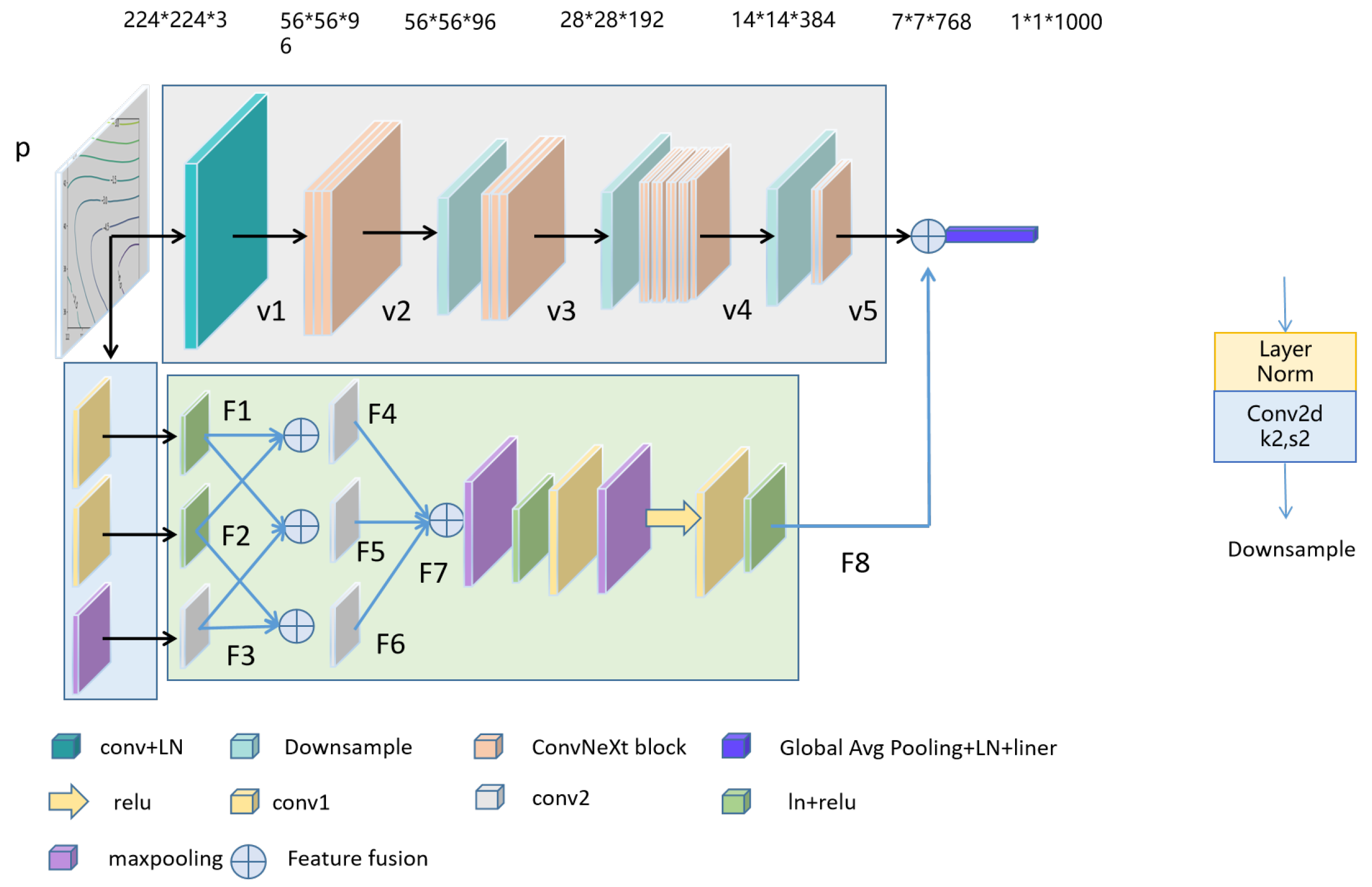
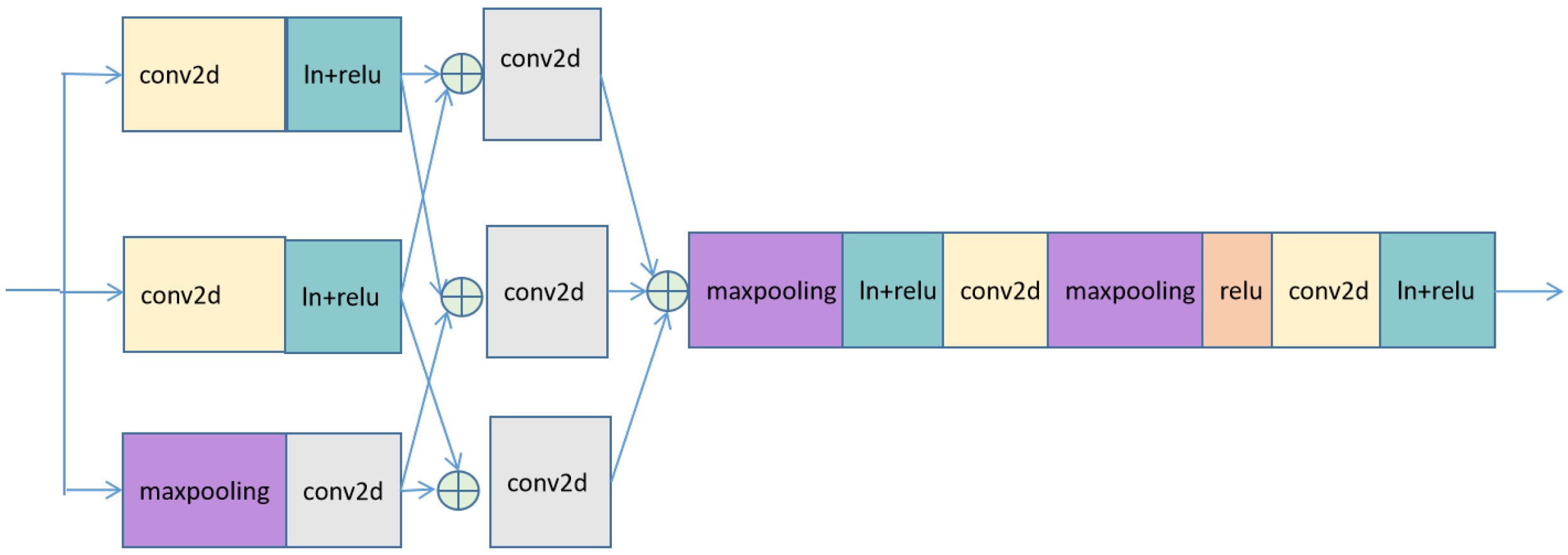
2.3.2. Principle and Network Structure of FConvNeXt

The network used in this experiment was the ConvNeXt-S model with a novel cross-fusion module for feature extraction. A schematic of the entire structure during execution is shown in Figure 4. The input variable of the model was a circulation field image with a size of 224 × 224 × 3. After being processed by the FConvNeXt network, the final output of the network was a vector of size 1 × 1 × 1000. The specific process is shown below.
The execution process in the ConvNeXt module consisted of five stages. The first stage: the original image (p) of size 224 × 224 × 3 was fed into a 4 × 4 convolutional layer and processed by layer normalization, resulting in a vector (v1) of size 56 × 56 × 96. The second stage: next, v1 was passed into a ConvNeXt module group consisting of 3 ConvNeXt modules (see Section 2.3.3). The output was a vector (v2) with a size of 56 × 56 × 96. The third stage: then, v2 was passed into a down-sampling layer, and then into a ConvNeXt module group with 3 ConvNeXt modules. The output was a vector (v3) with a size of 28 × 28 × 192. The processes in the fourth and fifth stages were similar to the process of the third stage, with the difference being that the fourth and fifth stages consisted of 9 and 3 ConvNext modules, respectively. They outputted vectors of size 14 × 14 × 384 (v4) and 7 × 7 × 768 (v5) respectively.
The execution process of the cross-fusion module was the following. Firstly, the original image (p) of size 224 × 224 × 3 was passed into 3 sets of convolutional layers. The first two sets consisted of a convolutional layer each, and the third set consisted of a max-pooling layer and a convolutional layer (as shown in the lower part of Figure 4). They, respectively, the vectors F1, F2, and F3 were output, which were 112 × 112 × 768 in size. Next, F1, F2, and F3 were cross-fused to obtain F4, F5, and F6 through convolutional layers, and then F4, F5, and F6 were fused to obtain the output feature vector F7 of size 112 × 112 × 768. For the next step, F7 was passed into a 2 × 2 max-pooling layer, which output a vector of size 56 × 56 × 768, followed by layer normalization and the ReLU activation function processing. It was passed through a 3 × 3 convolutional layer, outputting a vector of size 28 × 28 × 768, followed by a 2 × 2 max-pooling layer, outputting a vector of size 14 × 14 × 768; then, ReLU activation function processing was performed. It was then passed through another 3 × 3 convolutional layer, outputting a vector of size 7 × 7 × 768. After a final layer normalization and ReLU activation function processing, feature vector F8 was output.
The feature v5 was then added to F8, resulting in a feature vector of size 7 × 7 × 768. It was then globally average pooled and layer normalized, followed by linear layer processing. The final output result was a vector of size 1 × 1 × 1000.
In the down-sampling module, layer normalization was processed first, followed by a convolutional process, with the convolutional kernel size set to 2 and a step size of 2, as shown in Figure 4.
Layer normalization (LN) transformed the input features into data with a mean of 1 and a variance of 0, which was calculated as follows:
L N ( x i ) = α × ( x i μ ) σ 2 + ϵ + b
LN was the normalization of all features of each sample, and it ignored the size relationship between different samples and retained the size relationship between different features, where the mean is μ , the standard deviation is σ , and the parameters of LN are α and b.

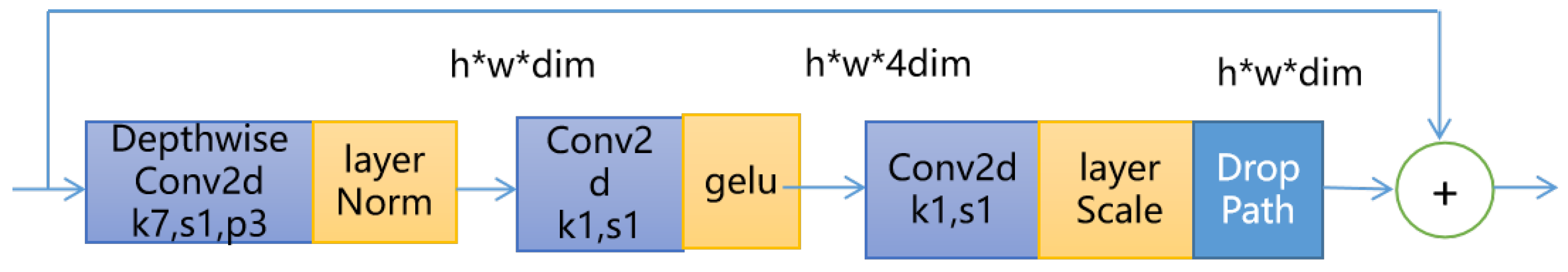
2.3.3. Introduction to the ConvNeXt Module

A key module in this network structure was the ConvNeXt module, which consisted of three main parts, as shown in Figure 5. The first was composed of a convolutional kernel of size 7, a convolutional operation with a padding of 3, and a layer normalization operation. The second part was composed of a convolutional operation of size 1 and an activation function. The third part consisted of a convolutional operation, a layer-scale operation, and a drop-path operation. The purpose of the drop-path operation was to discard some features at random, which could then reduce the probability of over-fitting. The final output was summed with the original output by applying the concept of a residual structure. The residual function could be described as a cell in which the original input is x. After a series of convolutional operations, the output function F(x) was obtained, whereupon the residual function H(x) = F(x) + x, and then it was activated by the GELU function. Its purpose was to prevent the partial loss of valid information in the original image as a result of a series of operations.

2.3.4. Introduction to the Cross-Fusion Feature Extraction Module

The main function of the cross-fusion feature extraction module was to improve the classification accuracy of the local circulation pattern. It consisted of two parts, as shown in Figure 6.
In the first half, feature y i = F i ( x ) was extracted in parallel through two convolutional operations and one max-pooling operation to obtain three output features. The three features were fused in pairs, and the results are shown in Formula (3). Then, the convolutional operation was carried out separately to process y i = F c ( y i ) ; finally, the three features were fused by Y = i = 1 3 y i to obtain Y. The initial convolutional operation was conducted to extract the initial information in the original image and retain more of the edge features. The max-pooling operation extracted the maximum features from the original image and only retained the most prominent features of the image. Then, two convolutional operations were used to extract features. As the features obtained by the max-pooling operation were the most prominent global features, this feature value was large, and the feature value obtained by the convolutional operation would be comparatively small. To narrow the feature value gap between the two results, two convolutional operations were used to increase the feature value. This was also critical for improving the accuracy of weak features.
y i = F i ( x ) i = 1 , 2 , 3
y 1 = y 1 + y 2 y 2 = y 1 + y 3 y 3 = y 2 + y 3
y i = F c ( y i ) i = 1 , 2 , 3
Y = i = 1 3 y i i = 1 , 2 , 3
The second half was devoted to further feature extraction using two max-pooling and two convolutional operations. The features were first extracted by a max-pooling operation, followed by a layer normalization and activation function operation, and finally by a convolutional operation. This operation was repeated later, and the final features were fused with the output of the ConvNeXt module.
We chose max-pooling for this step because it could preserve the strongest features of the image. Since the first half of the image was convoluted twice in parallel, the weak features also increased in value. An average-pooling operation would have blurred the features and increased the difficulty in distinguishing the differences between the weak features, and the previous parallel convolutional operation would not have improved the results further. Therefore, two max-pooling operations were finally selected as the methods used to process the features.

2.4. Experimental Design and Dataset Partitioning

This experiment focused on developing an objective discrimination method for the weather patterns corresponding to intense rainfalls in the Beijing–Tianjin–Hebei region. Various methods, such as ResNet, ConvNeXt, and FConvNeXt, have been used to perform fractal experiments and comparative analyses of the 500 hPa potential height field. The benchmark for comparison was the subjective classification described in Section 2.2.
To select the optimal parameters for our approach, we conducted several experiments and evaluated each method, selecting the results obtained during the best performance as the final outcome. Accordingly, the parameters obtained according to that result were used as the optimal parameters for that particular method. To ensure that the differences in the network structures were the main factor for obtaining different experimental results, hyper-parameters such as epochs, batch size, and initial learning rate were set equally. The optimal parameters were found by conducting many experiments and testing on the same set. For FConvNeXt, the optimal parameters were epochs = 50, batch size = 12, initial learning rate = 0.0005, and final learning rate = 0.00001.
In terms of the selection of activation functions, the ReLU activation function was used in the cross-fusion feature extraction module and in the final cross-fusion in FConvNeXt. In the ConvNeXt block, the GELU activation function was chosen because GELU is commonly used in activation functions in transformers. The construction idea of ConvNeXt refers to some concepts of transformers. In this study, we found that, regardless of using the GELU or the ReLU activation function, the final accuracy was not affected.
For the division of datasets, two sets of experimental schemes were used to validate the results. (1) The data from 1 May to 31 September 2013–2020 were randomly divided into a training set and a testing set with a ratio of 6:4. To better extract the system features with insignificant circulation fields, the potential height value was reduced by 100-fold overall. (2) The training set followed Scheme (1), and the data from 1 May–31 September 2021 were used as the testing set to prevent time leakage as well as to test the accuracy of the model’s results in Scheme (1).

2.5. Introduction to Evaluation Indicators

This section introduces the quality evaluation of the final classification results according to three aspects: classification accuracy, accuracy (ACC), and root-mean-squared error (RMSE). In this study, we used the subjective classification results as the ground truth.
Classification accuracy (the number of cases correctly identified by the objective method divided by the number of cases classified subjectively as the current type): the classification accuracy refers to the percentage of the testing set that the model correctly identified.
ACC (the proportion of correctly predicted samples by the classification model in all samples): ACC = (TP + TN)/(TP + TN + FP + FN), where TP represents true-positive; TN represents true-negative; FP represents false-positive; FN represents false-negative. Accuracy was mainly used to evaluate the model’s classification ability for all categories.
RMSE (root-mean-squared error): The root-mean-squared error (RMSE) is the square root of the mean of the square of all of the error values, and the use of the RMSE is very common. It is considered to be an excellent metric used to evaluate model performance. The computation method was Formula 6, where O i represents the observation value, G i represents the predicted value, and n is the total number of samples. RMSE reflects the degree of error between the predicted value and the true value; the smaller the value, the smaller the model’s prediction error and the better the performance.
R M S E = i = 1 n ( G i O i ) 2 i = 1 n i = 1 , 2 , 3 n
In this study, due to practical requirements, classification accuracy was the most important evaluation indicator, and this study used it as the primary reference indicator.

3. Results

3.1. Comparison of Multiple Objective Classification Methods

Table 1 shows the results of multiple machine learning methods for classifying heavy rainfall and flash flooding circulation patterns in the Beijing–Tianjin–Hebei region, comparing the overlap between the number of objectively classified cases and subjectively classified cases, which corresponded to each of the four subjective types. In addition, we conducted a separate classification accuracy analysis on the 2021 testing set to demonstrate the robustness of the model on new datasets.
When using the deep learning methods, the training and testing sets were divided according to the scheme in Section 2.4, with a split ratio of 6:4. As Table 1 shows, the accuracy of ResNet is lower than the accuracy of the other two methods for all four types, with LVT having the highest accuracy at 40%. Based on the data analysis, we found that ConvNeXt was significantly more accurate on the WSF and SPT types compared to ResNet, with an increase of 25% and 35.8%, respectively. In traditional deep learning, a significant improvement of 25% and 35.8% on an abundant amount of data would be considered remarkable.
Table 1 shows that the accuracy rates of FConvNeXt were 62.5%, 40%, 61%, and 14%, respectively. In the comparison between ResNet-50 and FConvNeXt, we found that FConvNeXt had significant improvements in accuracy (25% and 32.5% higher) during WSF and SPT classification compared to ResNet-50. In the comparison between ConvNeXt and FConvNeXt, FConvNeXt not only retained its high classification accuracy on WSF and SPT but also increased in accuracy on LVT, resulting in an accuracy value that was 14.3% higher compared to ConvNeXt. Overall, FConvNeXt was superior to ConvNeXt and ResNet in terms of accuracy.
FConvNeXt was shown to have the best results in terms of category accuracy, which was considered to be the most important metric for practical purposes. To further strengthen the study, the results of FConvNeXt, ConvNeXt, and ResNet on ACC is also presented in Table 2, Table 3 and Table 4. We obtained the ACC for the three correlations. Based on the experimental data, FConvNeXt had a much higher ACC on WSF than ConvNeXt and ResNet, with an increase of 7.2% over ConvNeXt and 6.4% over ResNet, indicating that ConvNeXt performed the worst in terms of ACC. In addition to the large gap in WSF, there were also significant differences in LVT_ACC among the three models, with ConvNeXt having the highest LVT_ACC, FConvNeXt ranking second, and ResNet differing by 9.6% from ConvNeXt. Interestingly, FConvNeXt, with the same high category accuracy as ResNet (40%) on LVT, appeared to be more stable in terms of ACC, suggesting that FConvNeXt performs well on different metrics. For SPT, FConvNeXt was similar to ConvNeXt, with a difference of only 0.8%, but ResNet differed significantly from the highest-performing ConvNeXt by 9.6%. On UTP, the three models had a similar performance, with FConvNeXt having the highest ACC. Overall, the data analysis showed that the total ACC of FConvNeXt was 73.8%; ConvNeXt’s total ACC was 72.4%; and ResNet’s total ACC was 67.4%. This indicates that FConvNeXt also showed the best performance in terms of the ACC index.
Further analyzing the RMSE, as shown in Table 5, each method had advantages. In terms of WSF, ResNet had the smallest error at only 0.08 km. This indicates that ResNet had the smallest error in the synthetic circulation pattern image. However, ResNet’s ACC and category accuracy were biased, which may have been due to the impact of the misclassification of other types of weather as WSF. However, FConvNeXt had the smallest RMSE on LVT and SPT, with values of 0.15 km and 0.14 km, respectively. In terms of UTP, ConvNeXt had the smallest RMS value of 0.12 km. These results indicate that FConvNeXt still had an advantage in RMS, with the smallest error for two types of weather, although ConvNeXt had the smallest error for UTP and ResNet had the smallest error for WSF.
Based on the comprehensive analysis of category accuracy, ACC, and RMSE, FConvNeXt had the best category accuracy and ACC, with significant improvements over ConvNeXt and ResNet. In terms of RMSE, FConvNeXt had a smaller advantage with a lower error than the other two methods. Based on these three aspects of the analysis, FConvNeXt was the optimal method.
In order to ensure that random data partitioning does not have too much of an impact on the experiments conducted in this study, we performed three sets of random data partitions, and the experimental results are shown in Table 6. The results show that the category accuracy of the three experiments in SPT is very close, ranging from 61% to 64%. In WSF, LVT, and UTP, the maximum difference is 11.5%, and the two groups (groups 1 and 3) are particularly similar. From the results of the three experiments, we can see that the results are stable with random data partitioning.

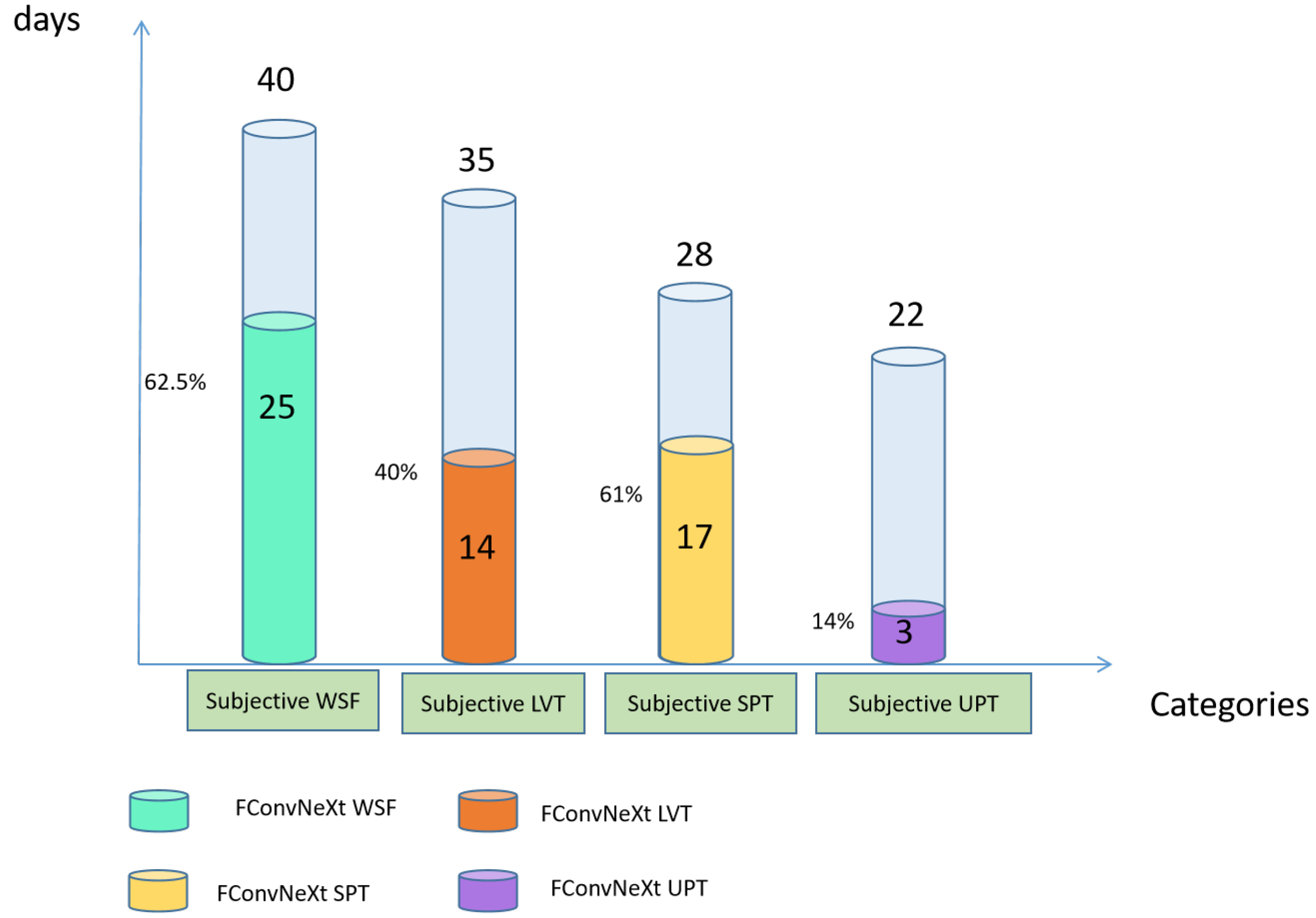
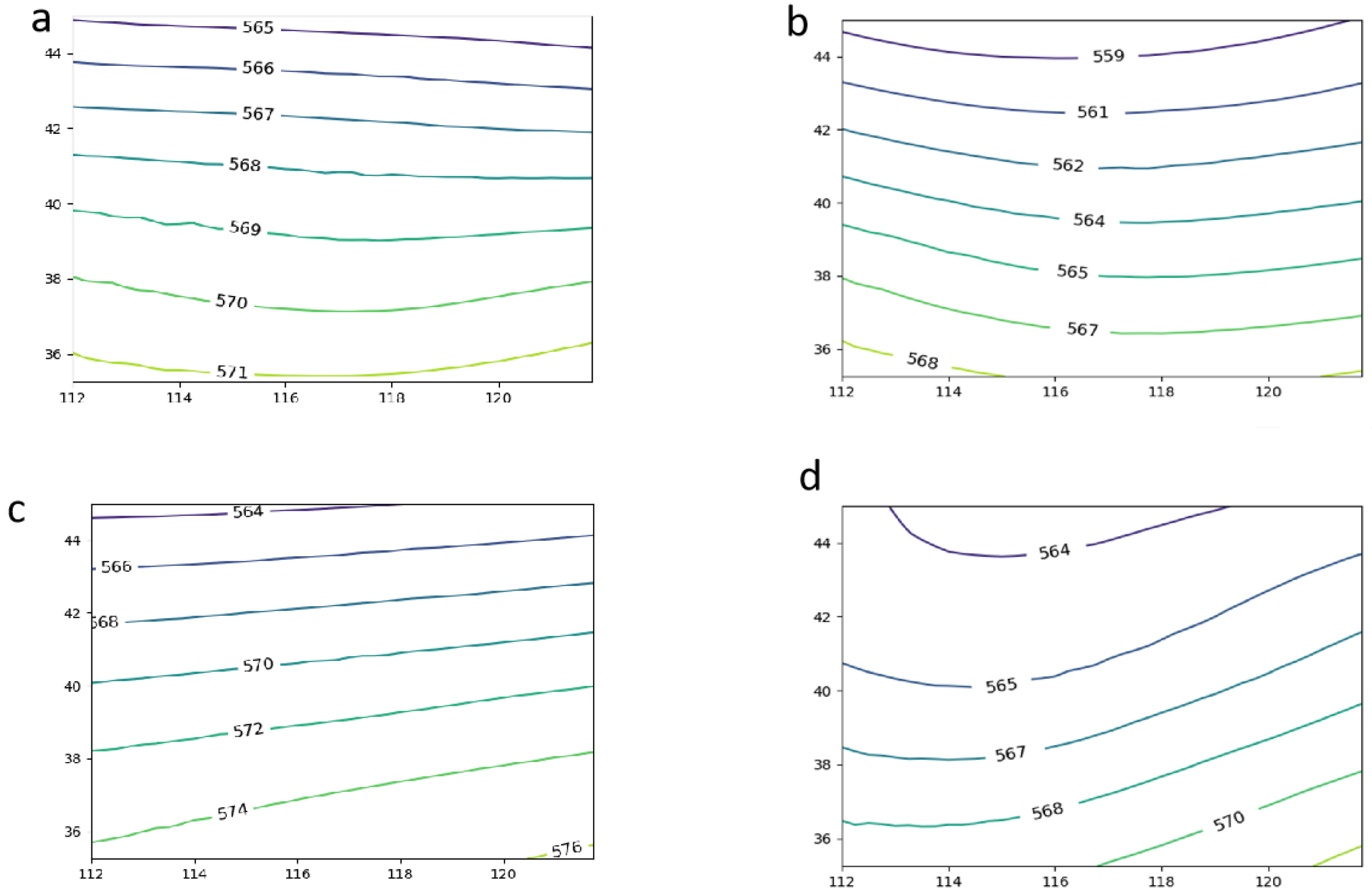
3.2. Circulation Pattern Classification by FConvNeXt

This section shows the classification details obtained using FConvNeXt. Figure 7 displays the classification results of FConvNeXt on the testing set, which were obtained in accordance with Table 1. The green bar shows that 25 cases of WSF have been identified in 40 cases. This is valuable information since WSF is difficult to identify even for forecasters because of its weak features when observed in a synoptic pattern. The SPT type also maintains a high accuracy rate of 61%.
When identifying LVT weather types, although the accuracy was only 40%, it still represented a significant improvement compared to the results of ConvNeXt, with an increase of 15%. As shown in Table 1, the recognition rate of LVT was relatively low in all methods. This is because the image information was incomplete and the features were not obvious; thus, the system display was incomplete. In the study area, the features of LVT and UTP were not fully displayed, so the LVT displayed as an incomplete low-vortex type and the UTP displayed as a high-altitude trough type with a shallow groove feature. These two were particularly prone to confusion, as shown in results f and h in Figure 2. Therefore, the classification accuracy of LVT was low.
To visualize the classification results of FConvNeXt more clearly and concisely, we presented the results in the form of a flat map, as illustrated in Figure 8. Although the distinction between LVT and UTP was lower in accuracy (as shown in Figure 8b,d), the circulation pattern maps showed significant differences. Its overall accuracy compared to the subjective classification method was 56%, and it had a characterized circulation pattern map of four categories. After testing the divided testing set, the classification results of each of the four categories on the testing set were synthesized. Many of the characteristics were relatively obvious, making it easier to distinguish the four kinds of circulation. As shown in Figure 8a, the circulation pattern map was partially flat with no major fluctuations, which is consistent with WSF’s characteristics (a relatively flat westerly band with no significant weather systems). Variations in vorticity are evident in Figure 8b. The vortex was distributed to the north and was effectively part of a complete northeast low vortex. Figure 8c shows a significant anticyclonic circulation in the southeast of the region, which belonged to a complete subtropical–high-pressure system. In Figure 8d, the northerly region had a clear UTP signature.
To facilitate a more intuitive comparison with the subjectively classified circulation patterns, we compared the diagrams of the subjectively classified patterns in Figure 3 with those in Figure 8. We found that the circulation pattern diagrams of FConvNeXt were similar to the subjectively classified circulation pattern diagrams, the vortex structure of LVT was consistent with the subjective classification results, and the slot structure of UTP in the northeast was also consistent with the subjective classification results. The vortex and slot features also corresponded to each other with roughly similar curvature lines in the circulation pattern diagram.
By comparing Figure 3 and Figure 8, we can see that Figure 8 is basically consistent with Figure 3 in terms of the feature distribution and structure. We can see that the contour density of Figure 3c and Figure 8c is closer, and both are dense in the north and sparse in the south. As shown in Figure 3b and Figure 8b, both have consistent features of a low vortex with clear vortex structures, and the position direction of the low vortex in both is also consistent. Compared to Figure 3d, the trough structure of Figure 8d is more obvious, but the contour density differs greatly, deviating from the actual observed value. In terms of WSF, both show consistent contour distributions with no significant fluctuations, and the contour density is also evenly distributed. Overall, the planar flow fields drawn by FConvNeXt were consistent with those of the real observation, demonstrating the superiority of FConvNeXt in weather classification.
To achieve the classification results for the test scenario Section 2.4, 40% of the dataset from 2013 to 2020 was used as test data. To test the applicability of the FConvNeXt classification, the independent 2021 flood period was used as the testing set for the classifications described in the next section.

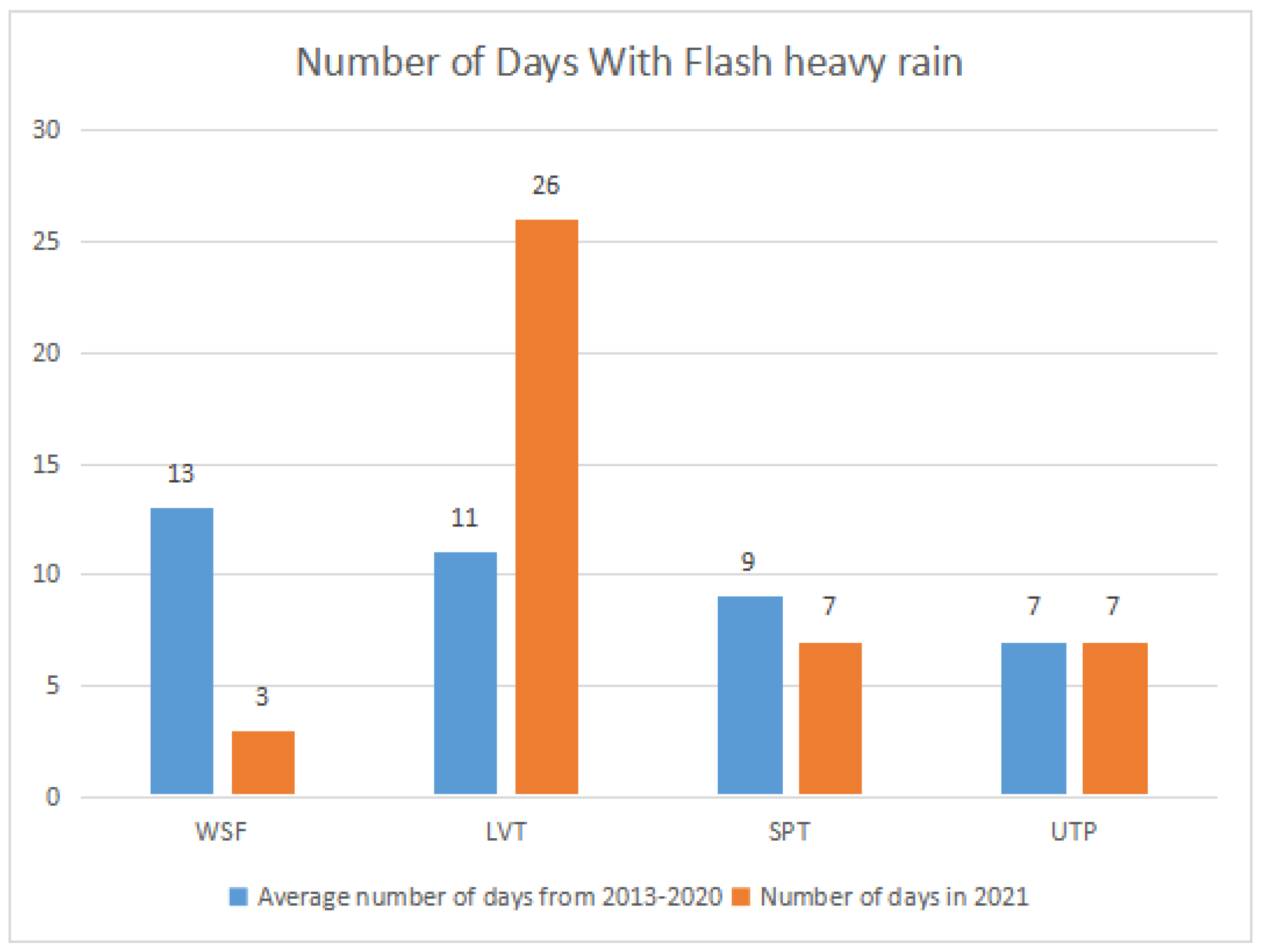
3.3. Performance of FConvNeXt in 2021 Test Set

We selected the flash rainfall events in 2021 as an independent testing set to evaluate the FConvNeXt model’s generalization ability by verifying future events using historical data. Since using historical data to predict future events is an important practical application, this section focuses on the results obtained from the 2021 testing set. The distribution of 2021 compared to the 2013–2020 multi-year mean (Figure 9) showed a significant difference. There was an obvious reduction in the WSF sample up to 3 days; a significant increase in LVT events up to 22 days; a slight reduction in SPT up to 7 days; and a flat UTP at 7 days. This difference in the sample distribution on the testing set poses a greater challenge for deep learning classification.
The classification results are shown in Figure 10. The accuracy for WSF was 66.6%; for LVT, it was 41%; for SPT, it was 29%; and for UTP, it was 14%. The accuracy of the WSF and LVT remained at 60% and 40%, respectively, but the accuracy of SPT was further reduced. The classification results show that there was greater confusion between LVT and UTP, with the three LVT cases being assigned to the UTP category, leading to more prominent low-vortex features in the UTP category. Furthermore, due to the easterly subtropical–high-pressure and the flatter system in the region of Beijing–Tianjin–Hebei, SPT and WSF were less recognizable, and four SPTs were instead categorized as WSFs.
To further validate our experimental results in a more scientific approach, we calculated the ACC (accuracy) for each category and combined it with the recall data (category accuracy) from Figure 10 for analysis.
As shown in Table 7, we obtained the ACC for each type of weather, resulting in an overall accuracy of 66.68%. In the WSF category, FConvNeXt achieved a recall rate of 67% and an accuracy of 57.8%, indicating that it correctly predicted the majority of results for this category’s samples. This suggests that FConvNeXt performed well in identifying critical features for this category’s samples. For the SPT and UTP categories, FConvNeXt achieved an accuracy of 75.6% and 80%, respectively, although the recall rates were relatively low. These results indicate that FConvNeXt predicted the majority of the correct results for these categories’ samples and had some recognition ability for crucial features of these categories. FConvNeXt’s overall classification accuracy of 66.68% indicates its ability to accurately classify all four categories without severe over- or under-fitting issues, demonstrating its good generalization ability.
Table 8 shows that LVT had the smallest RMSE of 0.102 km. Additionally, UTP had an error of 0.248 km. It had high ACC and a rather small RMSE when combined with low-category accuracy, which may have been because of the the similarity of UTP with LVT shown in the circulation plot in Figure 11. WSF and SPT tended to be confused in FConvNeXt, as shown in Figure 10, and they both had RMSE values larger than 0.3 km.
Correspondingly, the synthetic circulation pattern maps of the two were compared to assess the overlap between the results of the deep learning classification and the subjective classification. Figure 11 shows the circulation pattern map corresponding to the subjective classification in 2021, which had clear weather implications. Figure 11a shows the WSF circulation, in which there was no significant weather system forcing according to the local heavy convective precipitation events. The SPT (Figure 11c) shows a cyclonic circulation in the southeast of the region, which was the edge of a subtropical–high-pressure pattern that was intercepted in a limited area. The UTP (Figure 11d) shows a shallow trough system at the northeast of the region, which was actually the north part of the north–east low system.
Based on the b and d plots in Figure 11, we can observe that the features of LVT shown in the b plot are incomplete, as only a part is visible. However, the d plot shows a high-altitude trough with shallow trough features. It is quite evident from the plot that b and d have similar features, with similar curvatures and directions of the arcs. This is one of the reasons for the decrease in the accuracy of LVT and UTP in the test results of 2021 as, during testing, the model became confused between LVT and UTP, leading to misclassification and thereby reducing its accuracy.
Comparing Figure 11 with Figure 12a, we can see that the circulation pattern map in the WSF weather is, overall, a flat westerly band with no significant weather system pattern, which is more consistent with the subjective classification. Figure 12b shows the LVT with clear characteristics (prominent low-vortex features) of a significant vortex in the north of the region. The SPT in Figure 12c also largely reflects the characteristics of the southeastern anticyclonic circulation. These three flow patterns were more consistent with weather science significance, which indicates that the method successfully captured the features of incomplete vortex-influenced systems in a limited area with a non-significant weather system. In Figure 12d, a complete vortex system appears at the north of the UTP corresponding circulation pattern, indicating that it is a low-vortex circulation.This was due to three LVT cases being classified as UTP by the deep learning classification, whereas the other three UTPs were misclassified as LVTs. The reason for this issue was that this experiment studied the Beijing–Tianjin–Hebei region, and the primary influence system of LVT was the northeastern vortex. However, in limited areas, it was hard to present the complete northeastern vortex, and only the cyclonic flow pattern on its southern side could be shown. Therefore, it was easily confused with UTP, especially when the vortex curvature was not large enough.
Overall, the FConvNeXt classification of circulation patterns was largely reasonable, although less accurate, than the statistical results. The distribution of the four types of precipitation was examined to determine whether the precipitation distribution also differs significantly. The precipitation distribution corresponding to the subjective classification of the 2021 data (Figure 13) showed a significant difference between the four types, with each of their obvious precipitation distribution characteristics, which also corresponded to the circulation pattern map. WSF (Figure 13a) was more dispersed, with the main precipitation distributed in the three northern counties and Cangzhou, and scattered precipitation centers in the northwestern mountains in addition, which is more in line with the nature of WSF. LVT (Figure 13b) was influenced by the northeastern vortex system. Therefore, the intense rainfall was concentrated in the mountain-front areas below 500 m in the topography of the north-eastern Beijing–Tianjin–Hebei region. SPT (Figure 13c) occurred at the edge between the subtropical–high-pressure system and the western topography of the Beijing–Tianjin–Hebei region. The UTP (Figure 13d) centers were located in the pre-mountain and plain areas of Beijing–Tianjin and the pre-mountain areas of south-central Hebei.
Figure 14 shows the precipitation distribution corresponding to the classification results of FConvNeXt. The mountains had a blocking and directing effect on the water vapor from the ocean, so its influence on the precipitation in the Beijing–Tianjin–Hebei regions was reflected in the deep learning classification. LVT (Figure 14b) was the most consistent precipitation distribution in the category, as its fall zone was almost the same as the pattern observed in Figure 13b but with a weaker intensity. The WSF features were still evident in Figure 14a, with fragment precipitation events, and the main fall areas are represented in Figure 13a, but are weak in intensity. There was a significant deviation in the southwestern mountainous region of Hebei, since the error of the WSF precipitation map was caused by the four SPT cases that had been incorrectly assigned to this type. This was due to the lack of WSF cases in 2021 as well as the confusion between the two categories and their circulation patterns. UTP was difficult to distinguish from LVT in a limited area, resulting in three LVTs being misclassified as UTPs, so the precipitation distribution differed significantly from the subjective classification.
Based on the overall comparison of Figure 13 and Figure 14, the precipitation map generated by LVT was the best among the four types of results. The RMSE value of LVT, which was 0.102, indicates that it had the smallest error among the four types of weather. This study focused on short-term heavy rainfall classification in a limited area. The results were satisfactory whether analyzed from the circulation field map or the precipitation field map. The experimental results of FConvNeXt improved in different aspects compared to other methods, which proved that the cross-fusion feature extraction module was effective.

4. Discussion

Certain circulation configurations and different dominant weather systems generally cause precipitation with different properties and, accordingly, a specific distribution. In forecasting practices, precipitation forecasts are typically improved by identifying the corresponding circulation patterns. However, this relies on the forecaster’s judgment, which is highly subjective. There have been previous studies on objective weather identification, but they were focused on large-scale weather systems. However, catastrophic heavy rainfalls and flash flooding typically caused by meso- or smaller-scale weather systems are often highly localized over small areas, in which the weather system may not be fully presented. Similarly, the impact system may be weak and hard to detect and identify (e.g., a shallow trough), or there may even be no significant weather system (e.g., in local strong-convection cases). Therefore, the objective identification of weather patterns such as these is challenging, and little has been published on the topic. In this study, four types of circulation patterns corresponding to heavy rainfall and flash flooding in the Beijing–Tianjin–Hebei regions were taken as subjects. Three deep learning methods were tested. Our conclusions are as follows.
The deep learning solutions showed potential for the feature extraction of meso- or smaller-scale circulation patterns. ResNet was tested as a baseline. Then, ConvNeXt was introduced to categorize the weather patterns of local flash heavy rain. ConvNeXt fully used its residual structure to increase the number of convolutional layers while retaining more information on the original map to increase the accuracy of precipitation classification. It achieved significant improvements in the identification of the WSF and SPT types, but a decrease in the identification of the LVT type. Then, by introducing a cross-fusion feature extraction module, FConvNeXt was developed and tested. Based on the results of the ResNet, ConvNeXt, and FConvNeXt models, FConvNeXt performed the best. It maintained high accuracy on WSF and SPT tasks, achieving accuracy values of 62.5% and 61%, respectively. In addition, it displayed obvious improvements over ConvNeXt for LVT classification. The accuracy of the ConvNeXt model on the LVT task was 25.7%, whereas the improved version, FConvNeXt, had an accuracy of 40% on the same task. We also found that UPT is the most difficult type to identify, and the accuracy values achieved by ResNet, ConvNeXt, and FConvNeXt were all approximately 14%.
The study also used a strictly independent data set for the year 2021 to test the robustness of the model. It showed that the FConvNeXt classification accuracy maintained equal to if not even slightly better performances for WSF, LVT, and UPT, achieving values of 67%, 41%, and 14%, but a decrease in SPT was observed, with a value of 29%. A weather circulation plot was presented, and the presented plot matched with current meteorological understanding. Specific types of flow patterns also corresponded well with both the location and the intensity of the intense rainfall. However, we also found that FConvNeXt was prone to confusing UTP and LVT, as they have similar shallow trough features.
In summary, in contrast to previous objective classifications on large-scale weather systems in large regions, this study explored the objective classification of meso- and small-scale weather patterns that correspond to heavy rainfall and flash flooding within a limited region. Advanced deep learning models were employed that showed significant potential for this application. Furthermore, a new cross-fusion feature extraction module was proposed that improved the accuracy of the LVT classification within a limited region. Moreover, the study introduced a pre-training model to improve the training speed, which improved the accuracy and significantly shortened the training time.

Author Contributions

Writing—Original draft, L.J. and Q.Z.; resources, X.L.; conceptualization, X.W.; supervision, L.S.; software, Y.C. All authors have read and agreed to the published version of the manuscript.

Funding

This research was supported by the National Natural Science Foundation of China (Grant Nos. 41875058,41505079), the National Key R&D Project (Grant No. 2021YFC3000903), the CMA Innovation Foundation (CXFZ2023J001), the CMA weather review project (FPZJ2023-170), and the CMATC key research project (2022CMATCZD13).

Institutional Review Board Statement

Not applicable.

Informed Consent Statement

Not applicable.

Conflicts of Interest

The authors declare no conflict of interest.

Abbreviations

The following abbreviations are used in this manuscript:
WSFWeak Synoptic Forcing Type
LVTLow Vortex Type
SPTSubtropical-high Periphery Type
UTPUpper-level Trough Type
TPTTyphoon Type

References

  1. Yang, R.; Xing, P.; Du, W.; Dang, B.; Xuan, C.; Xiong, F. Climatic characteristics of precipitation in North China from 1961 to 2017. Sci. Geogr. Sin. 2020, 40, 1573–1583. [Google Scholar]
  2. Caracciolo, C.; Porcù, F.; Prodi, F. Precipitation classification at mid-latitudes in terms of drop size distribution parameters. Adv. Geosci. 2008, 16, 11–17. [Google Scholar] [CrossRef]
  3. Cai, J.; Tan, G.; Niu, R. Circulation pattern classification of persistent heavy rainfall in jianghuai region based on the transfer learning cnn model. J. Appl. Meteorol. Sci. 2021, 32, 233–244. [Google Scholar]
  4. Huth, R.; Beck, C.; Philipp, A.; Demuzere, M.; Ustrnul, Z.; Cahynová, M.; Kyselỳ, J.; Tveito, O.E. Classifications of atmospheric circulation patterns: Recent advances and applications. Ann. N. Y. Acad. Sci. 2008, 1146, 105–152. [Google Scholar] [CrossRef] [PubMed]
  5. Tveito, O.E. An assessment of circulation type classifications for precipitation distribution in Norway. Phys. Chem. Earth Parts A B C 2010, 35, 395–402. [Google Scholar] [CrossRef]
  6. Jia, L.; Li, W.; Chen, D.; An, X. A monthly atmospheric circulation classification and its relationship with climate in Harbin. Acta Meteorol. Sin. 2006, 64, 236–245. [Google Scholar]
  7. Bartoszek, K.; Skiba, D. Circulation types classification for hourly precipitation events in Lublin (East Poland). Open Geosci. 2016, 8, 214–230. [Google Scholar] [CrossRef]
  8. Deligiorgi, D.; Philippopoulos, K.; Kouroupetroglou, G. An Assessment of Self-Organizing Maps and k-Means Clustering Approaches for Atmospheric Circulation Classification. Recent Advances in Environmental Science and Geoscience. 17. 2014. Available online: https://www.inase.org/library/2014/venice/bypaper/ENVIR/ENVIR-01.pdf (accessed on 23 April 2023).
  9. Casado, M.; Pastor, M.; Doblas-Reyes, F. Links between circulation types and precipitation over Spain. Phys. Chem. Earth Parts A B C 2010, 35, 437–447. [Google Scholar] [CrossRef]
  10. Casado, M.; Pastor, M. Circulation types and winter precipitation in Spain. Int. J. Climatol. 2016, 36, 2727–2742. [Google Scholar] [CrossRef]
  11. Liu, R.; Sun, J.; Wei, J.; Fu, S. Classification of persistent heavy rainfall events over South China and associated moisture source analysis. J. Meteorol. Res. 2016, 30, 678–693. [Google Scholar] [CrossRef]
  12. Huth, R. Disaggregating climatic trends by classification of circulation patterns. Int. J. Climatol. J. R. Meteorol. Soc. 2001, 21, 135–153. [Google Scholar] [CrossRef]
  13. Bardossy, A.; Duckstein, L.; Bogardi, I. Fuzzy rule-based classification of atmospheric circulation patterns. Int. J. Climatol. 1995, 15, 1087–1097. [Google Scholar] [CrossRef]
  14. Zhao, Y.Y.; Zhang, Q.H.; Du, Y.; Jiang, M.; Zhang, J.P. Objective analysis of the extreme of circulation patterns during the 21 July 2012 torrential rain event in Beijing. Acta Meteorol. Sin. 2013, 71, 817–824. [Google Scholar]
  15. Hu, Y.; Ding, Y.; Liao, F. A classification of the precipitation patterns during the Yangtze-Huaihe meiyu period for the recent 52 years. Acta Meteorol. Sin. 2010, 68, 235–247. [Google Scholar]
  16. Lin, Y. Precipitation Regionalization Based on Fuzzy Clustering Algorithm. Meteorol. Sci. Technol. 2011, 39, 582–586. [Google Scholar]
  17. Zhou, X.; Sun, J.; Zhang, L.; Chen, G.; Cao, J.; Jie, B. Classification characteristics of continuous extreme rainfall events in North China. Acta Meteorol. Sin. 2020, 78, 761–777. [Google Scholar]
  18. Deng, A.; Tao, S.; Chen, L. The EOF analysis of rainfall in China during monsoon season. Chin. J. Atmos. Sci. 1989, 13, 289–295. [Google Scholar]
  19. Gao, S.H.; Cheng, M.M.; Zhao, K.; Zhang, X.Y.; Yang, M.H.; Torr, P. Res2net: A new multi-scale backbone architecture. IEEE Trans. Pattern Anal. Mach. Intell. 2019, 43, 652–662. [Google Scholar] [CrossRef]
  20. Feng, S.; Xiao, W. An Improved DBSCAN Clustering Algorithm. J. China Univ. Min. Technol. 2008, 37, 105–111. [Google Scholar]
  21. Dikbas, F.; Firat, M.; Koc, A.C.; Gungor, M. Classification of precipitation series using fuzzy cluster method. Int. J. Climatol. 2012, 32, 1596–1603. [Google Scholar] [CrossRef]
  22. Zhong, Q.; Sun, Z.; Chen, H.; Li, J.; Shen, L. Multi model forecast biases of the diurnal variations of intense rainfall in the Beijing–Tianjin–Hebei region. Sci. China Earth Sci. 2022, 65, 1490–1509. [Google Scholar] [CrossRef]
  23. Zhinian, Q.; Xueyuan, K.; Lihua, Z. Probe into the Forecast Based on Precipitation Types in After-flood Season of Guangxi. J. Guangxi Meteorol. 2002, 23, 9–11. [Google Scholar]
  24. Xinping, W.; Qing, Y.; Zhihui, L.; Hong, L.; Ligna, G. Fuzzy C-Means Clustering Method for Climatic Regionalization about Precipitation in Xinjiang. Desert Oasis Meteo 2013, 7, 30–35. [Google Scholar]
  25. Yang, L.; Deng, M. Based on k-means and fuzzy k-means algorithm classification of Precipitation. In Proceedings of the 2010 International Symposium on Computational Intelligence and Design, Hangzhou, China, 29–31 October 2010; Volume 1, pp. 218–221. [Google Scholar]
  26. Sun, J.; Liu, L.; Zhao, L. Clustering Algorithms Research. J. Softw. 2008, 19, 48–61. [Google Scholar] [CrossRef]
  27. Ostrovsky, Y.; Yanovsky, F. Use of neural network for turbulence and precipitation classification procedure. In Proceedings of the 2006 International Conference on Mathematical Methods in Electromagnetic Theory, Kharkiv, Ukraine, 26–29 June 2006; pp. 161–163. [Google Scholar]
  28. Liu, Z.; Mao, H.; Wu, C.Y.; Feichtenhofer, C.; Darrell, T.; Xie, S. A convnet for the 2020s. In Proceedings of the IEEE/CVF Conference on Computer Vision and Pattern Recognition, New Orleans, LA, USA, 18–24 June 2022; pp. 11976–11986. [Google Scholar]
  29. Hersbach, H.; Bell, B.; Berrisford, P.; Biavati, G.; Horányi, A.; Muñoz Sabater, J.; Nicolas, J.; Peubey, C.; Radu, R.; Rozum, I.; et al. ERA5 Hourly Data on Pressure Levels from 1979 to Present, Copernicus Climate Change Service (C3S) Climate Data Store (CDS); European Union: Brussels, Belgium, 2018. [Google Scholar]
  30. Shuai, S.; Chunxiang, S.; Yang, P.; Junxia, G.; Lei, B.; Chuancheng, S.; Shuai, H.; Jinsen, S. The lmproved Effects Evaluation of Three-Source Merged of Precipitation Products in China. Hydrology 2020, 15, 100129. [Google Scholar]
  31. Pan, Y.; Gu, J.; Yu, J.; Shen, Y.; Shi, C.; Zhou, Z. Test of merging methods for multi-source observed precipitation products at high resolution over China. Acta Meteorol. Sin. 2018, 76, 755–766. [Google Scholar]
  32. He, K.; Zhang, X.; Ren, S.; Sun, J. Deep residual learning for image recognition. In Proceedings of the IEEE Conference on Computer Vision and Pattern Recognition, Las Vegas, NV, USA, 27–30 June 2016; pp. 770–778. [Google Scholar]
  33. Targ, S.; Almeida, D.; Lyman, K. Resnet in resnet: Generalizing residual architectures. arXiv 2016, arXiv:1603.08029. [Google Scholar]
  34. Huang, G.; Liu, Z.; Van Der Maaten, L.; Weinberger, K.Q. Densely connected convolutional networks. In Proceedings of the IEEE Conference on Computer Vision and Pattern Recognition, Honolulu, HI, USA, 21–26 July 2017; pp. 4700–4708. [Google Scholar]
  35. Liu, P.; Zhang, H.; Zhang, K.; Lin, L.; Zuo, W. Multi-level wavelet-CNN for image restoration. In Proceedings of the IEEE Conference on Computer Vision and Pattern Recognition Workshops, Salt Lake City, UT, USA, 18–23 June 2018; pp. 773–782. [Google Scholar]
  36. Zagoruyko, S.; Komodakis, N. Wide residual networks. arXiv 2016, arXiv:1605.07146. [Google Scholar]
  37. He, Y.; Zhang, X.; Sun, J. Channel pruning for accelerating very deep neural networks. In Proceedings of the IEEE International Conference on Computer Vision, Venice, Italy, 22–29 October 2017; pp. 1389–1397. [Google Scholar]
  38. He, K.; Zhang, X.; Ren, S.; Sun, J. Delving deep into rectifiers: Surpassing human-level performance on imagenet classification. In Proceedings of the IEEE International Conference on Computer Vision, Santiago, Chile, 7–13 December 2015; pp. 1026–1034. [Google Scholar]
  39. Lin, T.Y.; Goyal, P.; Girshick, R.; He, K.; Dollár, P. Focal loss for dense object detection. In Proceedings of the IEEE International Conference on Computer Vision, Venice, Italy, 22–29 October 2017; pp. 2980–2988. [Google Scholar]
  40. Krizhevsky, A.; Sutskever, I.; Hinton, G.E. Imagenet classification with deep convolutional neural networks. Commun. ACM 2017, 60, 84–90. [Google Scholar] [CrossRef]
  41. Simonyan, K.; Zisserman, A. Very deep convolutional networks for large-scale image recognition. arXiv 2014, arXiv:1409.1556. [Google Scholar]
  42. Li, J.; Wang, C.; Huang, B.; Zhou, Z. ConvNeXt-backbone HoVerNet for nuclei segmentation and classification. arXiv 2022, arXiv:2202.13560. [Google Scholar]
Figure 1. Study area figure. (Longitude between 112°–122° east and latitude between 35°–45° north. The color bar represents colors and numbers that correspond to elevations on the map).
Atmosphere 14 00930 g001
Figure 2. The subjective circulation pattern classification results from 2013 to 2020 are shown in the figure, displaying the large-area distribution results in the region of east longitude (100°–130°) and north latitude (20°–55°). The categories displayed are WSF in (a), LVT in (b), SPT in (c), and UTP in (d). The red box in the figure defines the region of east longitude (112°–122°) and north latitude (35°–45°).
Atmosphere 14 00930 g002
Figure 3. The subjective circulation pattern classification results from 2013 to 2020 are shown in the figure, displaying the small-area distribution results in the region of east longitude (112°–122°) and north latitude (35°–45°). The categories displayed are WSF in (a), LVT in (b), SPT in (c), and UTP in (d).
Atmosphere 14 00930 g003
Figure 4. FConvNeXt network model. The top half is the ConvNeXt-S module, and the bottom half is the cross-fusion feature extraction module.
Atmosphere 14 00930 g004
Figure 5. Schematic diagram of the internal composition of the ConvNeXt module.
Atmosphere 14 00930 g005
Figure 6. Internal structure of the cross-fusion feature extraction module.
Atmosphere 14 00930 g006
Figure 7. FConvNeXt’s classification results on the testing set data from 2013 to 2020 compared to the overlap with the subjective classification (e.g., the first column: the light blue column indicates the total number of days of subjective WSF. Blue-green indicates the classification of 40 days of WSF, resulting in 25 days of WSF that overlap with the subjective WSF).
Atmosphere 14 00930 g007
Figure 8. The 2013–2020 FConvNeXt test set circulation pattern classification results: (a) WSF, (b) LVT, (c) SPT, (d) UTP.
Atmosphere 14 00930 g008
Figure 9. The 2021 subjective classified intense rainfall events versus those of the 2013–2020 average.
Atmosphere 14 00930 g009
Figure 10. FConvNeXt test results in 2021 (the first column: FConvNeXt WSF is indicated in blue-green. There are three days of subjective WSF, and the blue-green bars represent two days being correctly classified. The yellow bar represents one day of one SPT case being incorrectly identified as the WSF type).
Atmosphere 14 00930 g010
Figure 11. Circulation patterns of subjective classification for 2021 ((a) WSF, (b) LVT, (c) SPT, (d) UTP).
Atmosphere 14 00930 g011
Figure 12. Distribution of FConvNeXt test results in 2021 ((a) WSF, (b) LVT, (c) SPT, (d) UTP).
Atmosphere 14 00930 g012
Figure 13. Precipitation distribution of 2021 subjective classification results. ((a) WSF, (b) LVT, (c) SPT, and (d) UTP. The thick black line indicates the 500 m terrain height, and the thin black line indicates the 200 m terrain height).
Atmosphere 14 00930 g013
Figure 14. Precipitation distribution of FConvNeXt test results in 2021. ((a) WSF, (b) LVT, (c) SPT, (d) UTP. The thick black line indicates the 500 m terrain height, and the thin black line indicates the 200 m terrain height).
Atmosphere 14 00930 g014
Table 1. Accuracy results of deep learning classification trials.
Test MethodWSFLVTSPTUTP
ResNet-5037.5%40%28.5%13.6%
ConvNeXt62.5%25.7%64.3%14%
FConvNeXt62.5%40%61%14%
Table 2. FConvNeXt’s prediction results on the 2013–2020 testing set with true-positive (TP) cases (correctly predicted as positive), true-negative (TN) cases (correctly predicted as negative), false-positive (FP) cases (incorrectly predicted as positive), and false-negative (FN) cases (incorrectly predicted as negative).
Weather
Type
TPTNFPFNACC
WSF2556291564.8%
LVT1478122173.6%
SPT1782151179.2%
UTP39491977.6%
Table 3. ConvNeXt’s prediction results on the 2013–2020 testing set with true-positive (TP) cases (correctly predicted as positive), true-negative (TN) cases (correctly predicted as negative), false-positive (FP) cases (incorrectly predicted as positive), and false-negative (FN) cases (incorrectly predicted as negative).
Weather
Type
TPTNFPFNACC
WSF2547381557.6%
LVT98642676%
SPT1882151080%
UTP392121976%
Table 4. ResNet’s prediction results on the 2013–2020 testing set with true-positive (TP) cases (correctly predicted as positive), true-negative (TN) cases (correctly predicted as negative), false-positive (FP) cases (incorrectly predicted as positive), and false-negative (FN) cases (incorrectly predicted as negative).
Weather
Type
TPTNFPFNACC
WSF1558272558.4%
LVT1469212166.4%
SPT881162070.4%
UTP390131974.4%
Table 5. The RMSE results of ResNet, ConvNeXt, and FConvNeXt from 2013 to 2020.
Weather TypeWSFLVTSPTUTP
ResNet0.08 km0.19 km0.21 km0.16 km
ConvNeXt0.13 km0.17 km0.18 km0.12 km
FConvNeXt0.15 km0.15 km0.14 km0.19 km
Table 6. Accuracy of three sets of random tests.
Random
Sample
Grouping
WSFLVTSPTUTP
Group 162.5%40%61%14%
Group 252.5%49%64%5%
Group 360%37.5%61%14%
Table 7. FConvNeXt’s prediction results on the 2021 testing set with true-positive (TP) cases (correctly predicted as positive), true-negative (TN) cases (correctly predicted as negative), false-positive (FP) cases (incorrectly predicted as positive), and false-negative (FN) cases (incorrectly predicted as negative).
Weather
Type
TPTNFPFNACC
WSF22418157.8%
LVT91541753.3%
SPT2326575.6%
UTP1353680%
Table 8. The RMSE results from FConvNeXt from 2021.
Weather TypeWSFLVTSPTUTP
FConvNeXt0.343 km0.102 km0.307 km0.248 km
Disclaimer/Publisher’s Note: The statements, opinions and data contained in all publications are solely those of the individual author(s) and contributor(s) and not of MDPI and/or the editor(s). MDPI and/or the editor(s) disclaim responsibility for any injury to people or property resulting from any ideas, methods, instructions or products referred to in the content.

