

Bartlett–Lewis Model Calibrated with Satellite-Derived Precipitation Data to Estimate Daily Peak 15 Min Rainfall Intensity

Abstract
:1. Introduction
2. Data and Methods
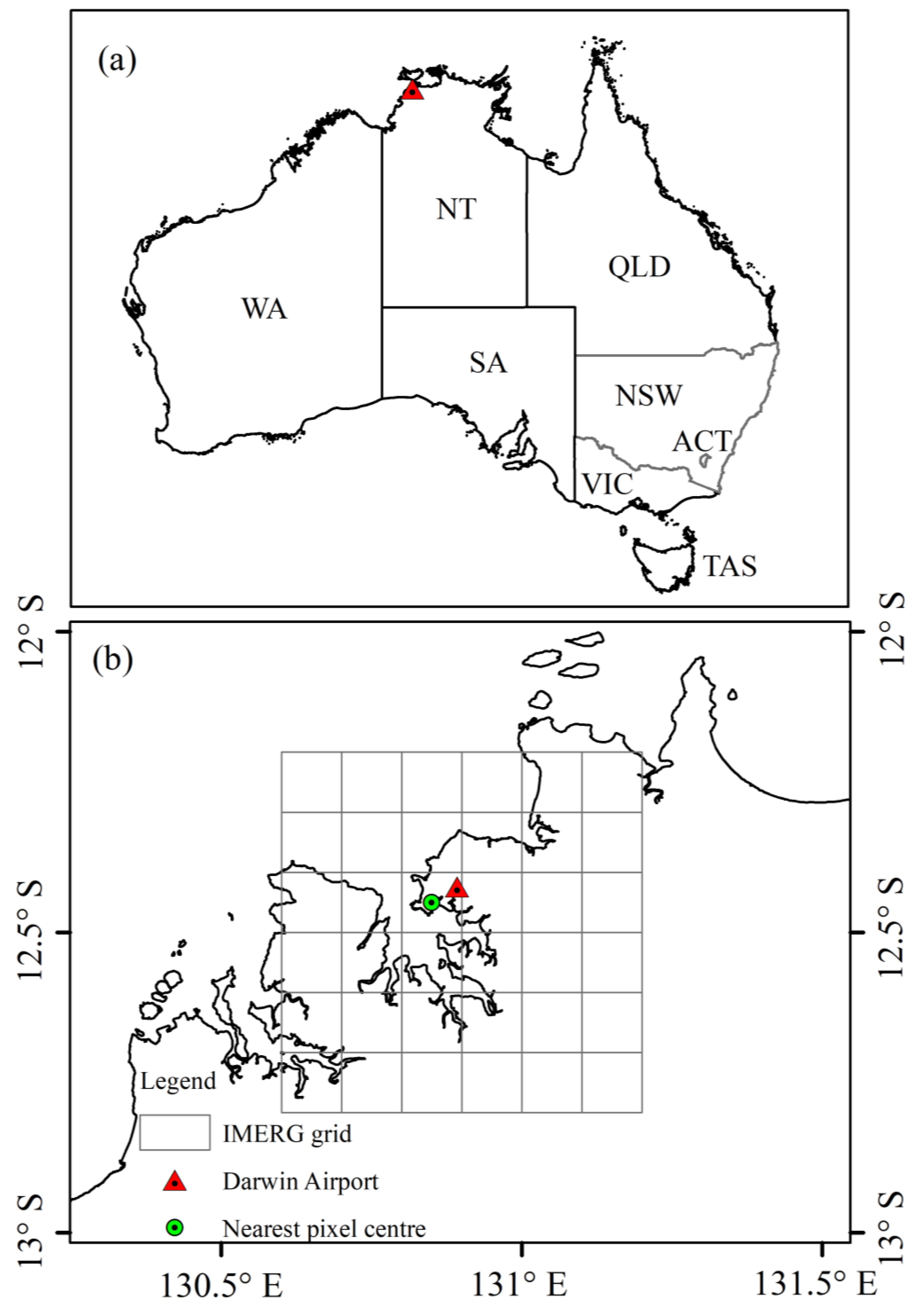
2.1. Pluviograph Data
2.2. Satellite-Derived Precipitation Products: IMERG
2.3. Model Descriptions
2.3.1. Fraser Model
2.3.2. Randomized Bartlett–Lewis Rectangular Pulse Model
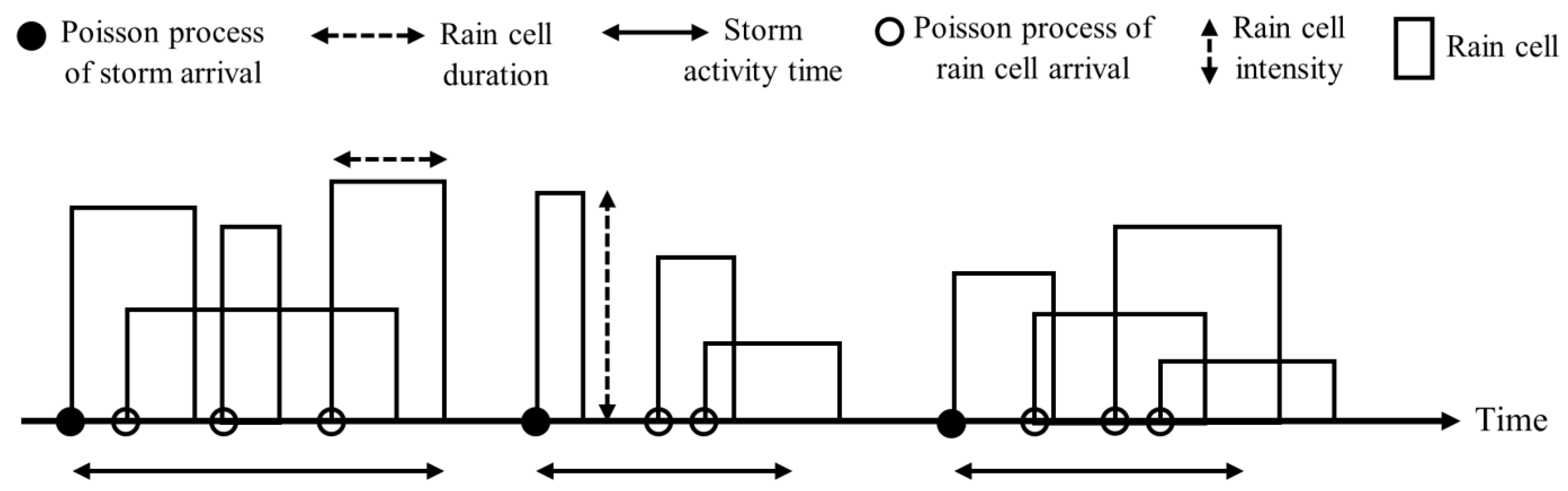
- Storms arrive (solid circles in Figure 2) according to a Poisson process with rate and each storm is associated with a random number of rain cells.
- Rain cell durations (width of the rectangles in Figure 2) follow the exponential distribution with parameter . The parameter is allowed to vary from storm to storm following the gamma distribution with shape parameter (unitless) and scale parameter and is used to determine the distributions of storm activity time, rain cell arrival, and rain cell depth.
- The storm activity time (solid double arrow lines in Figure 2) is an exponentially distributed random variable with parameter , where (unitless) is a model parameter.
- Rain cells arrive within a storm (open circles in Figure 2) according to a second Poisson process with rate , where (unitless) is a model parameter. The origin of the first rain cell within a storm always coincides with the storm origin. Further, rain cells can arrive only before the termination of the storm activity time.
- The rain cell intensity (height of the rectangles in Figure 2) follows either the exponential distribution with average cell depth or the gamma distribution with average cell depth and standard deviation , where and (unitless) are two model parameters.
Model Calibration
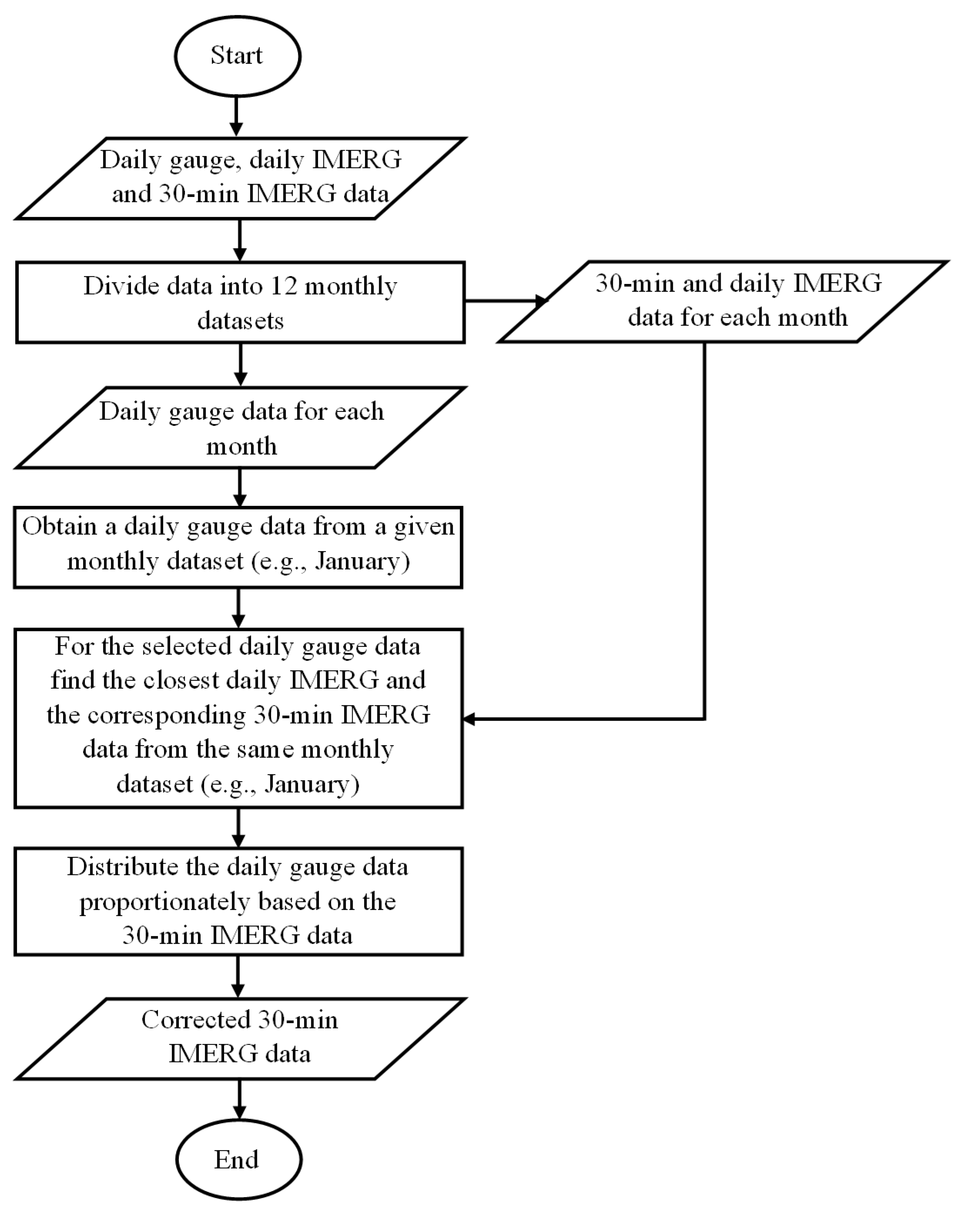
Disaggregation Scheme
- (a)
- The single- and multi-day wet periods, preceded and followed by one or more dry days, were obtained from the given daily pluviograph time series. The selected BLRP model (i.e., RBL-E or RBL-G) was used to generate storms associated with rain cells for each wet period at the 15 min timescale.
- (b)
- The intensities of the rain cells were generated for the modelled storms, and the generated daily rainfall depths were calculated to compare with the given daily depths using the following equation [12,28]:where and are the observed and generated rainfall depths in mm, respectively, for the th day in a wet period of days. A constant mm was used to avoid domination by the very low daily rainfall values. On the other hand, the logarithmic transformation was selected to prevent domination by the very high rainfall values. For each wet period, the process was repeated until the departure became lower than an allowable limit . The allowable departure was set to 0.1 as recommended by Kossieris, Makropoulos, Onof and Koutsoyiannis [12].
- (c)
- According to the proportional adjustment procedure, the generated sub-hourly rainfall depths for the th day in a wet period of days were modified as follows [12,28]:where and are the modified and generated rainfall depths in mm, respectively, for the th 15 min time interval of the th day in a wet period of days.
2.4. Performance Criteria
3. Results and Discussion
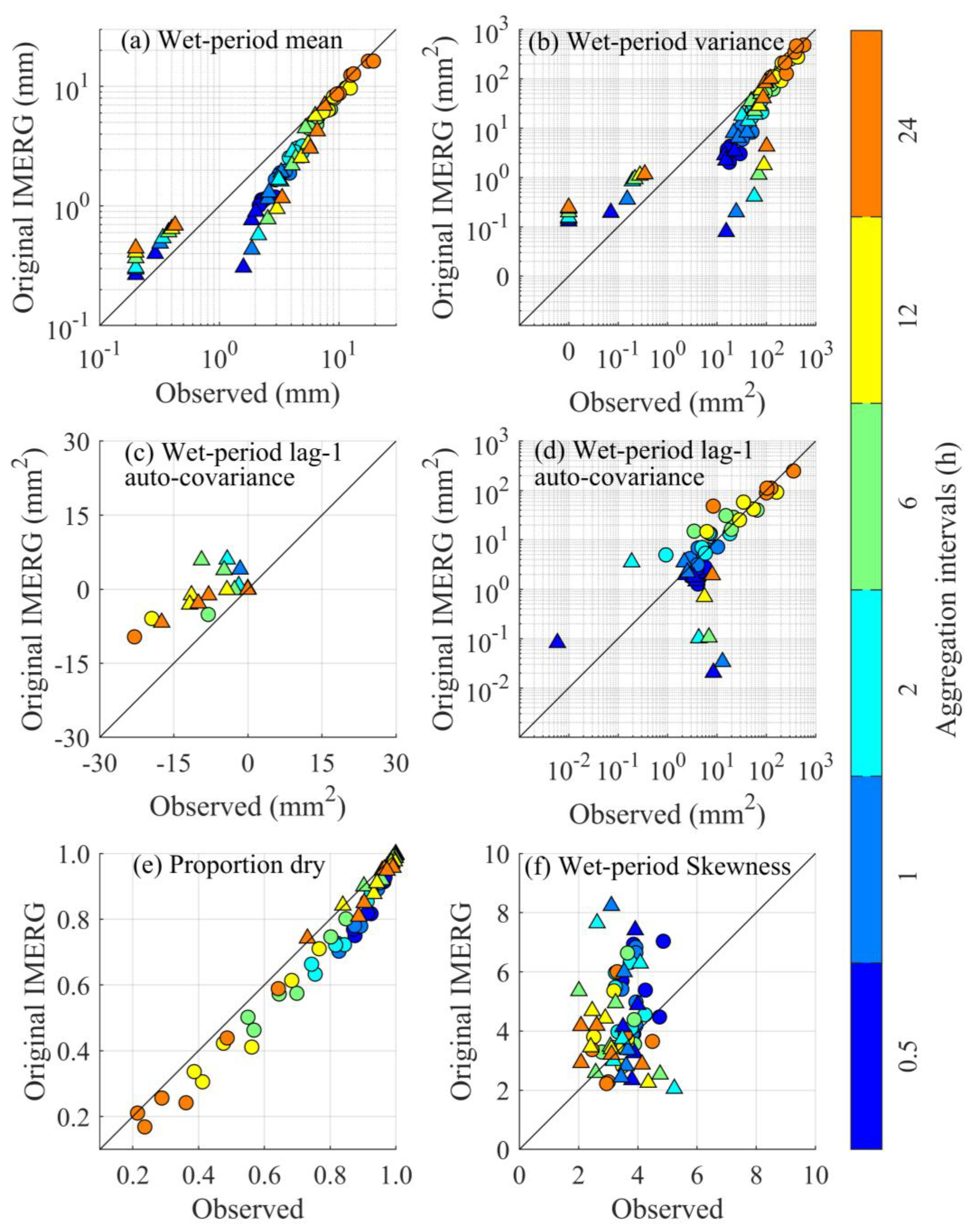
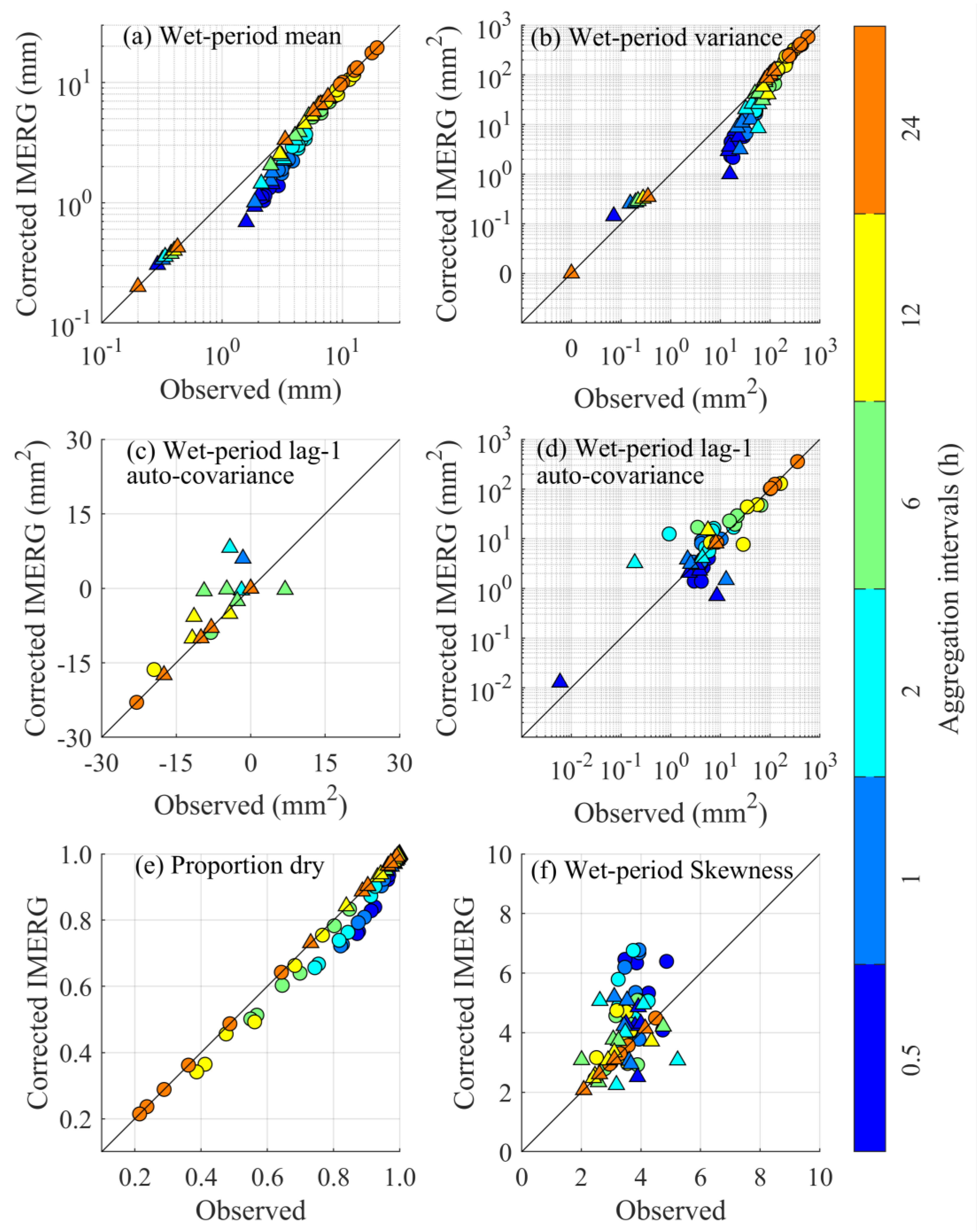
3.1. Comparison of IMERG with Pluviograph Statistics
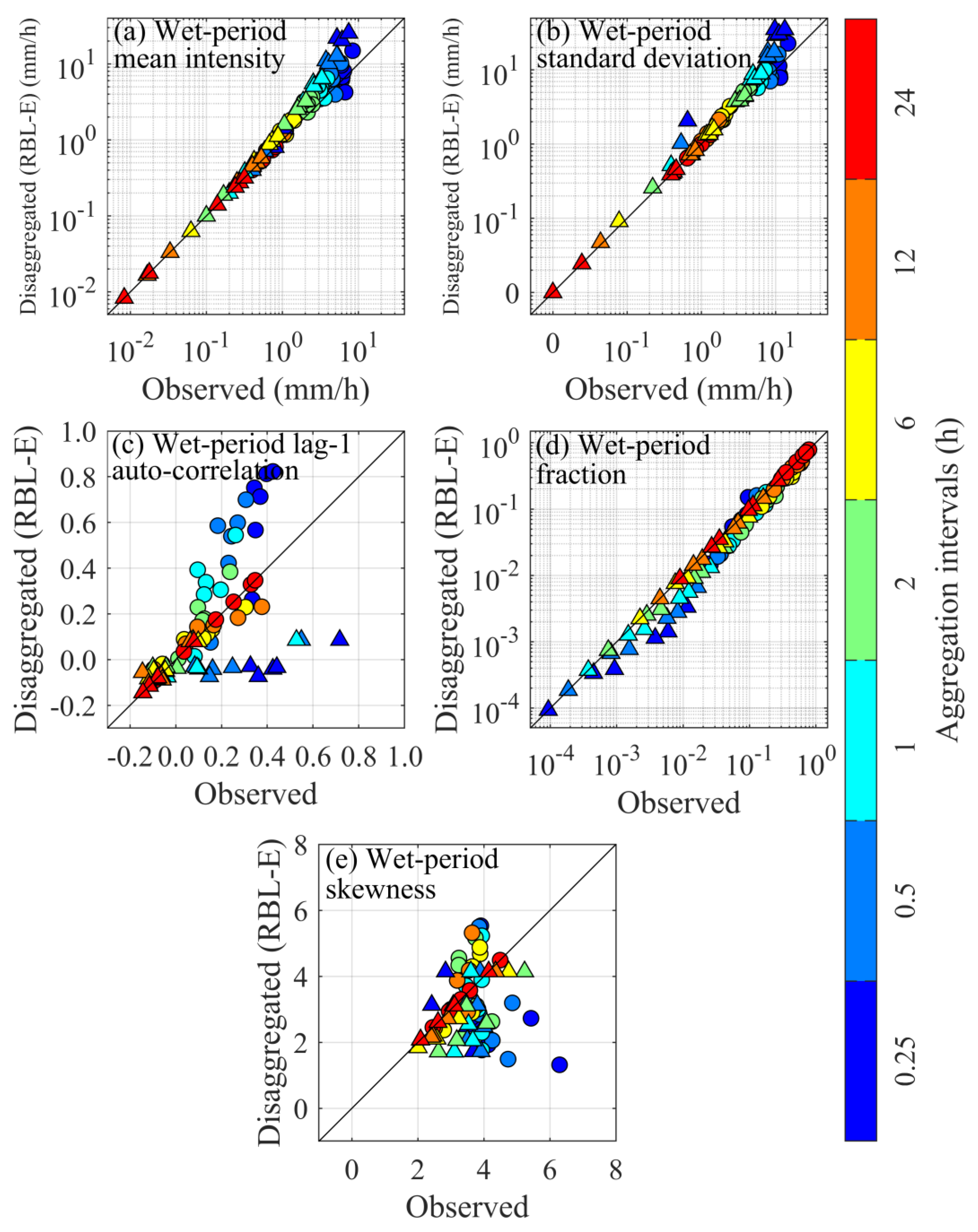
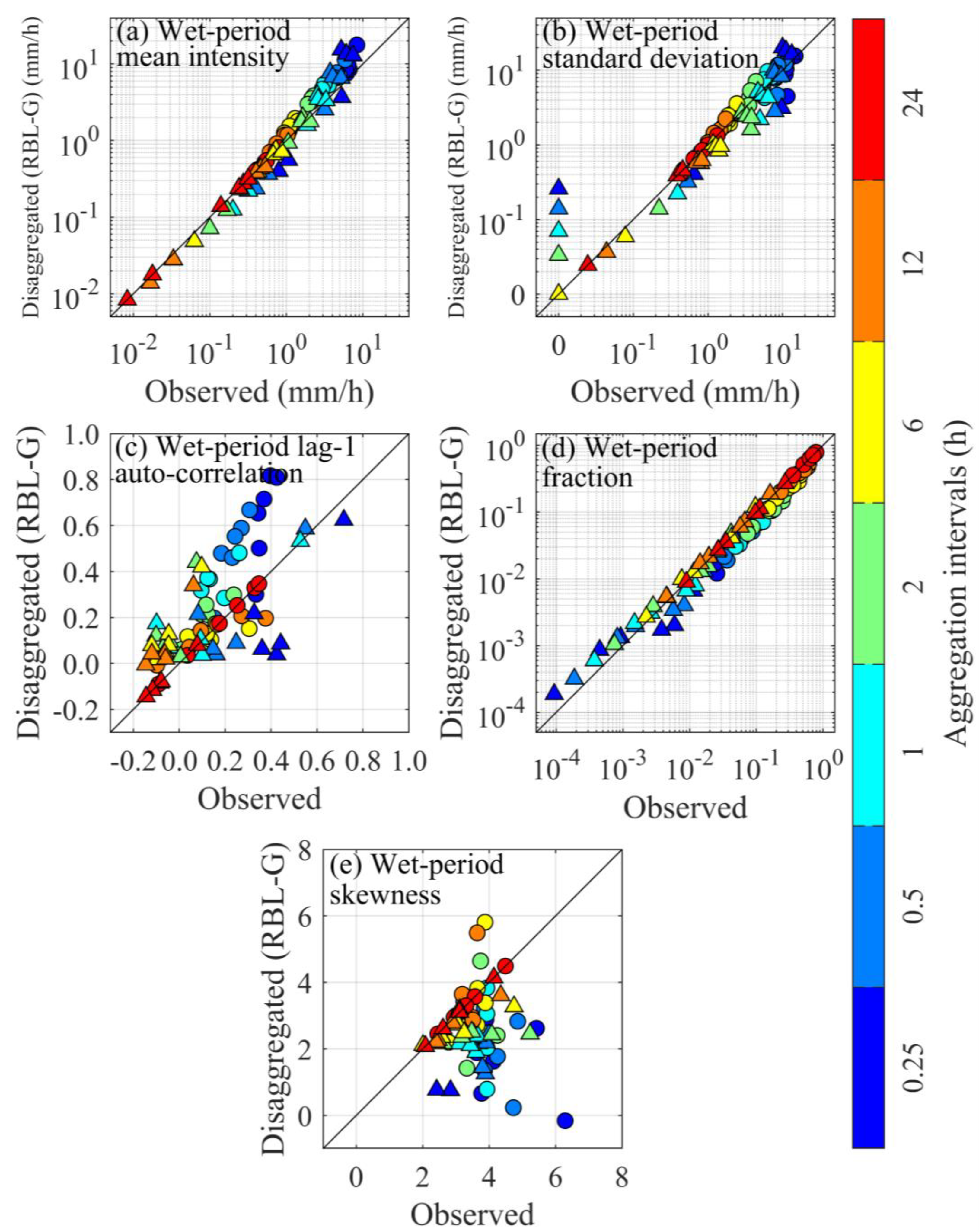
3.2. Comparison of Disaggregated with Pluviograph Statistics
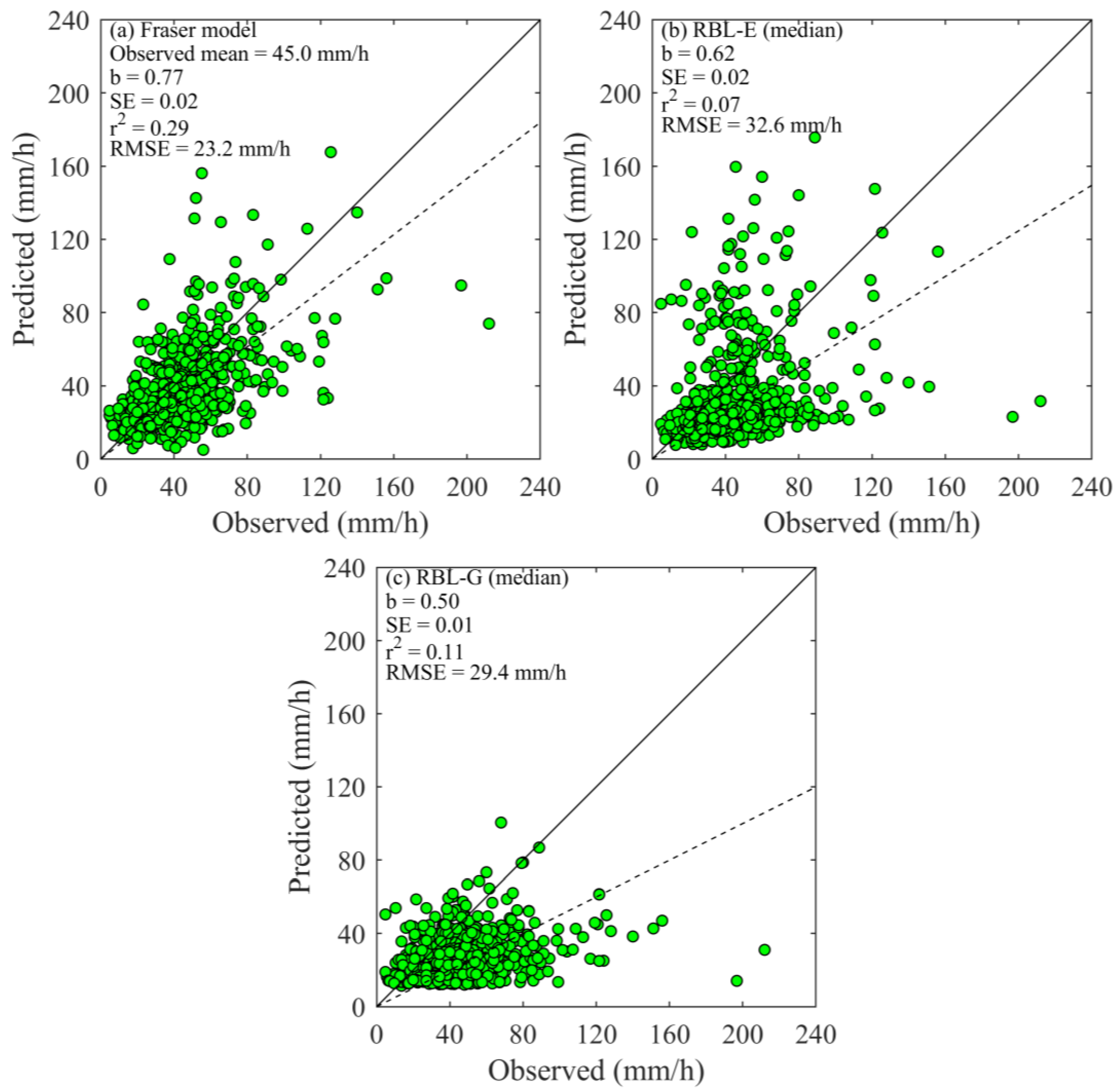
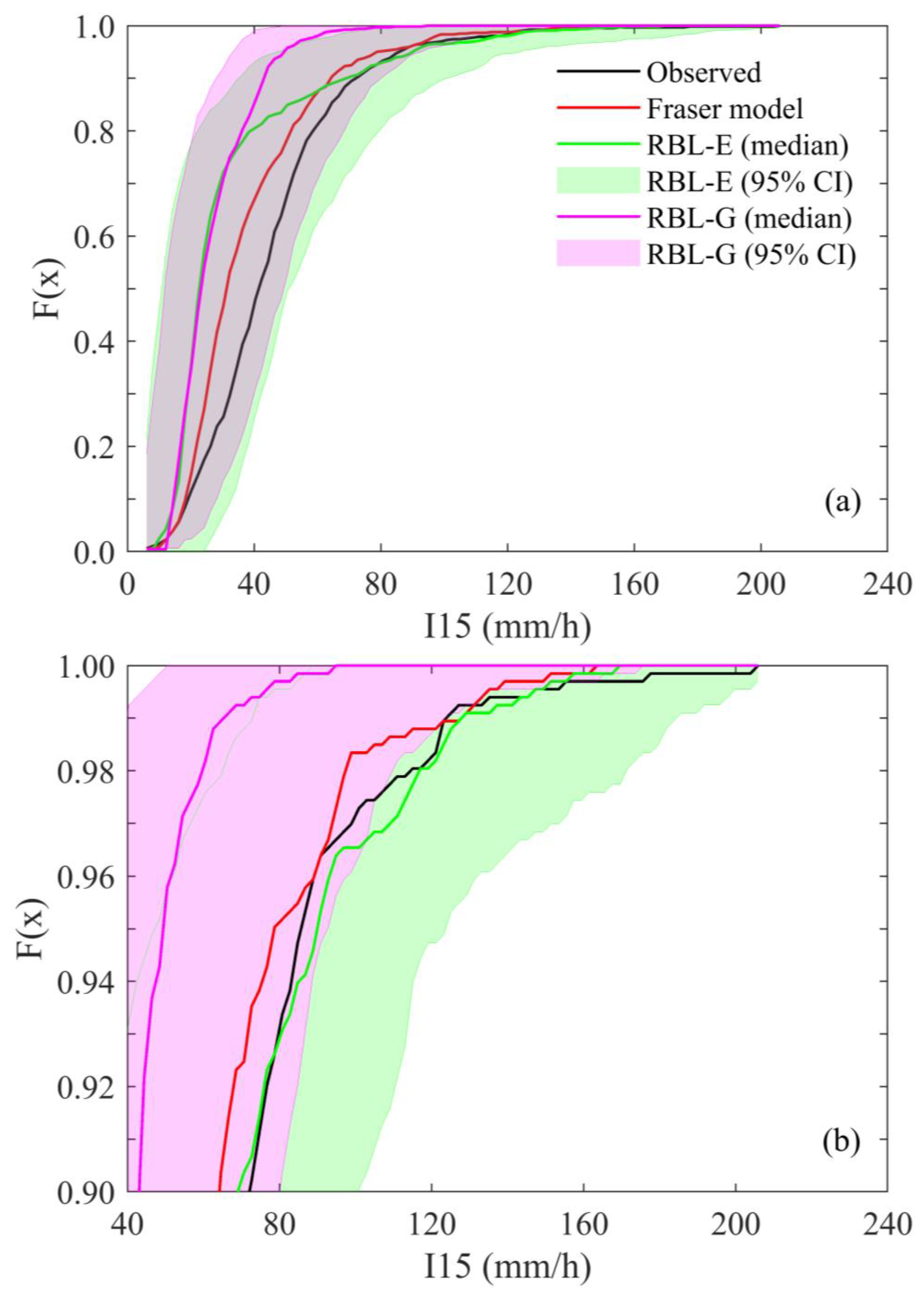
3.3. Comparison of Predicted with Observed I15
4. Summary and Conclusions
Author Contributions
Funding
Institutional Review Board Statement
Informed Consent Statement
Data Availability Statement
Acknowledgments
Conflicts of Interest
References
- Henry, B.; McKeon, G.; Syktus, J.; Carter, J.; Day, K.; Rayner, D. Climate Variability, Climate Change and Land Degradation. Clim. Land Degrad. 2007, 205–221. [Google Scholar] [CrossRef]
- McKeon, G.; Stone, G.; Ahrens, D.; Carter, J.; Cobon, D.; Irvine, S.; Syktus, J. Queensland’s Multi-Year Wet and Dry Periods: Implications for Grazing Enterprises and Pasture Resources. Rangel. J. 2021, 43, 121–142. [Google Scholar] [CrossRef]
- McKeon, G.M.; Stone, G.S.; Syktus, J.I.; Carter, J.O.; Flood, N.R.; Ahrens, D.G.; Bruget, D.N.; Chilcott, C.R.; Cobon, D.H.; Cowley, R.A.; et al. Climate Change Impacts on Northern Australian Rangeland Livestock Carrying Capacity: A Review of Issues. Rangel. J. 2009, 31, 1–29. [Google Scholar] [CrossRef] [Green Version]
- McKeon, G.M.; Hall, W.B.; Henry, B.K.; Stone, G.S.; Watson, I.W. Pasture Degradation and Recovery in Australia’s Rangelands: Learning from History; Queensland Department of Natural Resources, Mines and Energy: Brisbane, Australia, 2004. [Google Scholar]
- McKergow, L.A.; Prosser, I.P.; Hughes, A.O.; Brodie, J. Sources of Sediment to the Great Barrier Reef World Heritage Area. Mar. Pollut. Bull. 2005, 51, 200–211. [Google Scholar] [CrossRef]
- Rickert, K.G.; Stuth, J.W.; McKeon, G.M. Modelling Pasture and Animal Production. In Field and Laboratory Methods for Grassland and Animal Production Research; ‘t Mannetje, L., Jones, R.M., Eds.; CABI Publishing: New York, NY, USA, 2000. [Google Scholar] [CrossRef]
- Scanlan, J.C.; Pressland, A.J.; Myles, D.J. Run-Off and Soil Movement on Mid-Slopes in North-East Queensland Grazed Woodlands. Rangel. J. 1996, 18, 33–46. [Google Scholar] [CrossRef]
- Green, J.; Johnson, F.; Beesley, C.; The, C. Rainfall Estimation: Design Rainfall. In Australian Rainfall and Runoff: A Guide to Flood Estimation; Ball, J., Babister, M., Nathan, R., Weeks, W., Weinmann, E., Retallick, M., Testoni, I., Eds.; Commonwealth of Australia (Geoscience Australia): Barton, ACT, Australia, 2019. [Google Scholar]
- Fraser, G.W.; Carter, J.O.; McKeon, G.M.; Day, K.A. A New Empirical Model of Sub-Daily Rainfall Intensity and Its Application in a Rangeland Biophysical Model. Rangel. J. 2011, 33, 37–48. [Google Scholar] [CrossRef]
- Jeffrey, S.J.; Carter, J.O.; Moodie, K.B.; Beswick, A.R. Using Spatial Interpolation to Construct a Comprehensive Archive of Australian Climate Data. Environ. Model. Softw. 2001, 16, 309–330. [Google Scholar] [CrossRef]
- Islam, A.; Yu, B.; Cartwright, N. Coupling of Satellite-Derived Precipitation Products with Bartlett-Lewis Model to Estimate Intensity-Frequency-Duration Curves for Remote Areas. J. Hydrol. 2022, 609, 127743. [Google Scholar] [CrossRef]
- Kossieris, P.; Makropoulos, C.; Onof, C.; Koutsoyiannis, D. A Rainfall Disaggregation Scheme for Sub-Hourly Time Scales: Coupling a Bartlett-Lewis Based Model with Adjusting Procedures. J. Hydrol. 2018, 556, 980–992. [Google Scholar] [CrossRef] [Green Version]
- Kaczmarska, J.; Isham, V.; Onof, C. Point Process Models for Fine-Resolution Rainfall. Hydrol. Sci. J. 2014, 59, 1972–1991. [Google Scholar] [CrossRef] [Green Version]
- Cross, D.; Onof, C.; Winter, H.; Bernardara, P. Censored Rainfall Modelling for Estimation of Fine-Scale Extremes. Hydrol. Earth Syst. Sci. 2018, 22, 727–756. [Google Scholar] [CrossRef] [Green Version]
- Park, J.; Cross, D.; Onof, C.; Chen, Y.; Kim, D. A Simple Scheme to Adjust Poisson Cluster Rectangular Pulse Rainfall Models for Improved Performance at Sub-Hourly Timescales. J. Hydrol. 2021, 598, 126296. [Google Scholar] [CrossRef]
- Huffman, G.J.; Stocker, E.F.; Bolvin, D.T.; Nelkin, E.J.; Tan, J. Gpm Imerg Final Precipitation L3 Half Hourly 0.1 Degree X 0.1 Degree V06; Goddard Earth Sciences Data and Information Services Center (GES DISC): Greenbelt, MD, USA, 2019. [Google Scholar] [CrossRef]
- Huffman, G.J.; Bolvin, D.T.; Braithwaite, D.; Hsu, K.-L.; Joyce, R.J.; Kidd, C.; Nelkin, E.J.; Sorooshian, S.; Stocker, E.F.; Tan, J.; et al. Integrated Multi-Satellite Retrievals for the Global Precipitation Measurement (Gpm) Mission (Imerg). In Satellite Precipitation Measurement; Levizzani, V., Kidd, C., Kirschbaum, D.B., Kummerow, C.D., Nakamura, K., Turk, F.K., Eds.; Springer International Publishing: Cham, Switzerland, 2020; pp. 343–353. [Google Scholar] [CrossRef]
- Tan, J.; Huffman, G.J.; Bolvin, D.T.; Nelkin, E.J. Imerg V06: Changes to the Morphing Algorithm. J. Atmos. Ocean. Technol. 2019, 36, 2471–2482. [Google Scholar] [CrossRef]
- Rodriguez-Iturbe, I.; Cox, D.R.; Isham, V. Some Models for Rainfall Based on Stochastic Point-Processes. Proc. R. Soc. Lond. Ser. A-Math. Phys. Sci. 1987, 410, 269–288. [Google Scholar] [CrossRef]
- Rodriguez-Iturbe, I.; Cox, D.R.; Isham, V. A Point Process Model for Rainfall—Further Developments. Proc. R. Soc. Lond. Ser. A-Math. Phys. Sci. 1988, 417, 283–298. [Google Scholar] [CrossRef]
- Onof, C.; Wang, L.-P. Modelling Rainfall with a Bartlett-Lewis Process: New Developments. Hydrol. Earth Syst. Sci. 2020, 24, 2791–2815. [Google Scholar] [CrossRef]
- Cowpertwait, P.; Isham, V.; Onof, C. Point Process Models of Rainfall: Developments for Fine-Scale Structure. Proc. R. Soc. A Math. Phys. Eng. Sci. 2007, 463, 2569–2587. [Google Scholar] [CrossRef]
- Ugray, Z.; Lasdon, L.; Plummer, J.; Glover, F.; Kelly, J.; Martí, R. Scatter Search and Local Nlp Solvers: A Multistart Framework for Global Optimization. INFORMS J. Comput. 2007, 19, 328–340. [Google Scholar] [CrossRef]
- Kim, D.; Onof, C. A Stochastic Rainfall Model That Can Reproduce Important Rainfall Properties across the Timescales from Several Minutes to a Decade. J. Hydrol. 2020, 589, 125150. [Google Scholar] [CrossRef]
- Wheater, H.S.; Chandler, R.E.; Onof, C.J.; Isham, V.S.; Bellone, E.; Yang, C.; Lekkas, D.; Lourmas, G.; Segond, M.-L. Spatial-Temporal Rainfall Modelling for Flood Risk Estimation. Stoch. Environ. Res. Risk Assess. 2005, 19, 403–416. [Google Scholar] [CrossRef]
- Kaczmarska, J.M.; Isham, V.S.; Northrop, P. Local Generalised Method of Moments: An Application to Point Process-Based Rainfall Models. Environmetrics 2015, 26, 312–325. [Google Scholar] [CrossRef] [Green Version]
- Freitas, E.d.S.; Coelho, V.H.R.; Xuan, Y.; Melo, D.d.C.; Gadelha, A.N.; Santos, E.A.; Galvão, C.d.O.; Filho, G.M.R.; Barbosa, L.R.; Huffman, G.J.; et al. The Performance of the Imerg Satellite-Based Product in Identifying Sub-Daily Rainfall Events and Their Properties. J. Hydrol. 2020, 589, 125128. [Google Scholar] [CrossRef]
- Koutsoyiannis, D.; Onof, C. Rainfall Disaggregation Using Adjusting Procedures on a Poisson Cluster Model. J. Hydrol. 2001, 246, 109–122. [Google Scholar] [CrossRef]
- R Core Team. R: A Language and Environment for Statistical Computing; R Foundation for Statistical Computing: Vienna, Austria, 2020. [Google Scholar]
- Ombadi, M.; Nguyen, P.; Sorooshian, S.; Hsu, K. Developing Intensity-Duration-Frequency (Idf) Curves from Satellite-Based Precipitation: Methodology and Evaluation. Water Resour. Res. 2018, 54, 7752–7766. [Google Scholar] [CrossRef]


| b (SE) | ||||
|---|---|---|---|---|
| Parameter | Original IMERG | Corrected IMERG | Original IMERG | Corrected IMERG |
| Wet-period mean (mm) | 0.81 (0.02) | 0.93 (0.01) | 0.96 | 0.98 |
| Wet-period variance (mm2) | 0.71 (0.02) | 0.97 (0.01) | 0.93 | 0.99 |
| Wet-period lag-1 auto-covariance (mm2) | 0.73 (0.02) | 0.96 (0.01) | 0.93 | 0.98 |
| Proportion dry | 0.95 (0.01) | 0.97 (0.00) | 0.97 | 0.98 |
| Wet-period skewness | 1.21 (0.06) | 1.17 (0.04) | 0.00 | 0.23 |
| b (SE) | ||||
|---|---|---|---|---|
| Parameter | RBL-E | RBL-G | RBL-E | RBL-G |
| Wet-period mean intensity (mm/h) | 1.84 (0.10) | 1.60 (0.05) | 0.70 | 0.88 |
| Wet-period standard deviation (mm/h) | 1.54 (0.09) | 1.03 (0.04) | 0.69 | 0.78 |
| Wet-period lag-1 auto-correlation | 0.84 (0.10) | 1.10 (0.09) | 0.31 | 0.49 |
| Wet-period fraction | 0.92 (0.01) | 0.90 (0.01) | 0.98 | 0.97 |
| Wet-period skewness | 0.84 (0.04) | 0.69 (0.04) | 0.03 | 0.00 |
Disclaimer/Publisher’s Note: The statements, opinions and data contained in all publications are solely those of the individual author(s) and contributor(s) and not of MDPI and/or the editor(s). MDPI and/or the editor(s) disclaim responsibility for any injury to people or property resulting from any ideas, methods, instructions or products referred to in the content. |
© 2023 by the authors. Licensee MDPI, Basel, Switzerland. This article is an open access article distributed under the terms and conditions of the Creative Commons Attribution (CC BY) license (https://creativecommons.org/licenses/by/4.0/).
Share and Cite
Islam, M.A.; Yu, B.; Cartwright, N. Bartlett–Lewis Model Calibrated with Satellite-Derived Precipitation Data to Estimate Daily Peak 15 Min Rainfall Intensity. Atmosphere 2023, 14, 985. https://doi.org/10.3390/atmos14060985
Islam MA, Yu B, Cartwright N. Bartlett–Lewis Model Calibrated with Satellite-Derived Precipitation Data to Estimate Daily Peak 15 Min Rainfall Intensity. Atmosphere. 2023; 14(6):985. https://doi.org/10.3390/atmos14060985
Chicago/Turabian StyleIslam, Md. Atiqul, Bofu Yu, and Nick Cartwright. 2023. "Bartlett–Lewis Model Calibrated with Satellite-Derived Precipitation Data to Estimate Daily Peak 15 Min Rainfall Intensity" Atmosphere 14, no. 6: 985. https://doi.org/10.3390/atmos14060985