Non-Equilibrium Turbulent Transport in Convective Plumes Obtained from Closure Theory

Abstract

The non-equilibrium property of turbulence modifies the characteristics of turbulent transport. With the aid of response function formalism, such non-equilibrium effects in turbulent transport can be represented by the temporal variation of the turbulent energy (K) and its dissipation rate ($\epsilon$) along the mean stream through the advective derivatives of K and $\epsilon$. Applications of this effect to the turbulent convection with plumes are considered for the first time in this work. The non-equilibrium transport effects associated with plumes are addressed in two aspects. Firstly, the effect associated with a single plume is evaluated using data measured in the recent plume/jet experiments. The second argument is developed for the collective turbulent transport associated with multiple plumes mimicking the stellar convection zone. In this second case, for the purpose of capturing the plume motions into the advective derivatives, use has to be made of the time–space double-averaging procedure, where the turbulent fluctuations are divided into the coherent or dispersion component (which represents plume motions) and the incoherent or random component. With the aid of the transport equations of the coherent velocity stress and the incoherent counterpart, the interaction between the dispersion and random fluctuations are also discussed in the context of convective turbulent flows with plumes. It is shown from these analyses that the non-equilibrium effect associated with plume motions is of a great deal of relevance in the convective turbulence modeling.

1. Introduction

Turbulent flows encountered in astro/geophysical phenomena as well as laboratory plasma ubiquitously have huge Reynolds numbers. Since the direct numerical simulations (DNSs) of such flows are impossible in the foreseeable future, the turbulence or subgrid-scale (SGS) modeling approach provides a powerful tool for analyzing turbulent flows in these phenomena.

In conventional turbulence modeling, the simple expressions of turbulent fluxes such as the eddy viscosity and eddy diffusivity representations are very useful and have been extensively utilized [1]. For instance, the turbulent momentum flux, defined by the Reynolds stress, is modeled by the turbulent transport coefficients, eddy viscosity, coupled with the mean velocity strain. The eddy viscosity is expressed in terms of the quantities that characterize the dynamics and statistical properties of the turbulence. In the mixing-length formulation, the eddy viscosity ${\nu }_{\mathrm{T}}$ is expressed by the characteristic turbulent velocity v and length scale ℓ as ${\nu }_{\mathrm{T}}={\nu }_{\mathrm{T}}(v,\mathsf{\ell })$. In the standard K–$\epsilon$ model, ${\nu }_{\mathrm{T}}$ is modeled in terms of the turbulent kinetic energy K and its dissipation rate $\epsilon$ as ${\nu }_{\mathrm{T}}={\nu }_{\mathrm{T}}(K,\epsilon )$. As compared with the mixing-length formulation, the K–$\epsilon$ is more elaborated since the dynamics of the turbulent fields and their interaction with the mean fields are taken into account through the transport equations of K and $\epsilon$ [2,3].

In spite of the notable achievements of simple gradient-diffusion-type models for turbulent fluxes with the eddy viscosity and eddy diffusivity representations, several situations exist wherein such models would completely fail. One such deficiency appears when the eddy viscosity model is applied to a situation with cross-flow configuration. This failure is caused by the lack of vorticity or rotation effects in the eddy viscosity model. An alleviation of this deficiency of the eddy viscosity model was proposed with the aid of an analytical statistical theory of inhomogeneous turbulence applied to a non-reflectional symmetric system with an emphasis on the helicity effects [4,5]. Another kind of deficiency shows up in the case of turbulence with non-equilibrium properties. For instance, in homogeneous-shear turbulence, the evaluation of the eddy viscosity systematically fails because of the overestimates of the turbulent energy K and its dissipation rate $\epsilon$. There, the energy injection increases with time, and the energy dissipation process cannot catch up with the injection at the energy-containing scale. This is caused by the non-equilibrium property of turbulence induced by the energy injection due to the flow shear. In order to alleviate this flaw in the framework of the K–$\epsilon$ model with the eddy viscosity representation, the non-equilibrium effect has to be incorporated into the eddy viscosity representation [6].

Employing the response function formalism in turbulence closure studies provides a powerful way to construct a self-consistent turbulence theory without resorting to any parameter. There are several classical modern theories of turbulence closure [7,8,9,10]. Starting with the Liouville equation derived by Edwards [8], Herring [9,10] constructed a series of self-consistent field (SCF) theories for turbulence closure. In the formulation, the coupled equations of the two-time velocity correlation function and the response function are derived under the requirement that the probability distribution functions satisfy the self-consistency condition. The obtained equations for the correlation and response functions are similar to the those obtained with the direct-interaction approximation (DIA) by Kraichnan [7]. In the combination of the DIA with multiple-scale analysis, we address the convective turbulence with variable density and velocity shear. One important consequence of this multiple-scale DIA analysis lies in the point that it enables us to treat the non-equilibrium effect of turbulence through the Lagrangian derivative of the turbulence fields. If turbulence properties such as the turbulent energy K and its dissipation rate $\epsilon$ are spatially developing in the streamwise direction, the non-equilibrium effects are represented by the advective derivatives of K and $\epsilon$, $(\mathbf{U}·\mathsf{\nabla })K$ and $(\mathbf{U}·\mathsf{\nabla })\epsilon$ in the Lagrangian derivatives. In the model for the homogeneous-shear turbulent flow [6], the non-equilibrium properties of turbulence including the variations in the time and length scales of turbulence are taken into account in the expression of the eddy viscosity through the Lagrangian derivative along the mean velocity $\mathbf{U}$ of the turbulent energy and its dissipation rate as ${\nu }_{\mathrm{T}}={\nu }_{\mathrm{T}}(K,\epsilon ,DK/Dt,D\epsilon /Dt)$ where $D/Dt=\partial /\partial t+\mathbf{U}·\mathsf{\nabla }$.

There are several types of buoyant streams in nature. Some buoyant flows are purely driven by thermobuoyancy (plumes) and others are driven by a combination of thermobuoyancy and dynamical forcing (thermobuoyant jets, non-isothermal shear layers). In the buoyancy-dominated turbulent flows, the turbulent convection is well represented by large-scale plumes [11,12,13,14]. In order for a turbulence model to treat turbulent convective flows, the turbulence interaction with coherent structures such as a large-scale jet and plume has to be properly represented in the model. Because of the presence of jets and plumes, the turbulent fluxes deviate from the usual gradient diffusivity, viscosity, etc. [14]. The turbulent transport coefficients should properly reflect such coherent structure effects. Another example in astrophysics can be seen in supernova explosion studies. In the core-collapse supernovae (CCSNe) explosion problem, turbulent effects aid the relaunch of blast shock waves due to the neutrino heating [15,16,17,18,19,20,21]. In order to identify the turbulence effects most relevant to the explosion condition, Murphy and Meakin [21] extensively examined several types of closure models. By comparing the model simulation results with the 2D simulation counterparts, they found that the standard turbulent flux models based on the gradient-transport approximation failed to reproduce the turbulent transport of the mass, momentum and heat in the stellar interiors. This suggests that the buoyancy-dominated flows of core-collapse convection are characterized by large-scale plumes. The entrainment between the rising and sinking plumes strongly affects the transport properties of neutrino-driven turbulence. In particular, the turbulent dissipation, which is balanced by the buoyancy drive, is dominantly controlled by the entrainment of negatively buoyant plumes.

It has been theoretically and experimentally shown that the dissipation rates in jets and plumes follow the Kolmogorov equilibrium law only if their spreading rates do not vary with the streamwise distance [22,23]. Adopting the Lie symmetry group theory on the statistical turbulent model equations, Sunita and Layek [24] recently argued the case of non-equilibrium turbulent dissipation in buoyant axisymmetric plumes in unstratified stagnant ambient at the infinite-Reynolds-number limit. They considered the relationship between the dissipation rates of the turbulent kinetic energy and turbulent thermal fluctuation, and the entrainment coefficients in the Kolmogorov and non-Kolmogorov regions of turbulent dissipations. They showed that the well-known link between entrainment and dissipation in the Kolmogorov region of turbulence is also established in the non-Kolmogorov region.

As mentioned above, with the aid of the response function formalism, the non-equilibrium properties of plume motions can be expressed by the variations in the turbulent kinetic energy and its dissipation rate along the plume motions. Recent elaborated laboratory experiments with jets and negatively or positively buoyant plumes provide detailed data on the spatial distributions of the turbulent energy and its dissipation rate as well as the jet and plume velocity distributions [25,26,27,28]. Utilizing these data, we can evaluate the variation of the turbulent energy and its dissipation rate along the jet/plume motion. Such an evaluation enables us to examine how much non-equilibrium effect may be present in turbulent flows associated with the jet and plume. This is one of the novel points discussed in this work.

Negatively or positively buoyant plumes play a dominant role in mass, momentum and heat mixing in the stellar convection zone. In the stellar convection zone case, we have to simultaneously treat the effects of numerous plumes on the turbulent fluxes, such as the turbulent mass flux, momentum flux and heat or internal-energy flux, in the mean-field equations. The non-equilibrium effect associated with these numerous plumes is investigated with the aid of the numerical simulations of a simplified domain mimicking the stellar convection zone. A turbulence model incorporating the non-equilibrium effect into the expressions of the turbulence fluxes should be validated in comparison with the direct numerical simulations (DNSs) of the turbulent mass, momentum and heat or internal-energy fluxes. In order to properly capture the effects of plume motions, which are part of fluctuating motions in the framework of the mean-field modeling, we introduce some elaborated averaging procedures in this evaluation of the non-equilibrium turbulence model. This is a time–space double-averaging procedure, which has been recently applied to a stellar convection zone [29]. This point will also be discussed in this paper.

The organization of this paper is as follows. In Section 2, we present the mean-field equations with the turbulence correlations, which should be expressed in terms of the mean-field and transport coefficients representing the statistical properties of turbulence. In Section 3, closure models for the turbulent fluxes are promoted with the aid of their theoretical derivations, with special reference to the corrections to the conventional gradient-transport approximations. There, modifications due to the non-equilibrium effects are presented. In Section 4, the roles of the non-equilibrium effects are suggested in the context of recent plume/jet experiments. In Section 5, the role of the plumes in the turbulent transport is discussed in the context of the stellar convection. In addition, the interaction between the coherent and incoherent fluctuations is argued for using the transport equations of each component of fluctuation energy. Concluding remarks are given in Section 6.

2. Equations of Compressible Hydrodynamic Turbulence

The material of this work is plumes in compressible convective turbulence. The turbulent fluxes, such as the turbulent mass flux, the Reynolds stress, the turbulent heat, or internal-energy flux, in the mean-field equations are analyzed with the aid of the two-scale direct-interaction approximation (TSDIA) formulation. In this method, the response or Green’s function is used to incorporate the non-equilibrium properties of the turbulence along the mean or grid-scale (GS) flow into the turbulent transport coefficients. By applying the present formulation to the statistical analysis of the turbulent transports in the presence of numerous plumes, a time–space double-averaging procedure is adopted. Since there is no general way of determining the time-domain filtering, we have to make use of the physical considerations on the plume statistics and dynamics including its lifetime for determining the filter in the time domain. This point should be further explored beyond the present formulation described below.

2.1. Mean-Field Equations and Turbulent Correlations

We adopt the conventional Reynolds decomposition procedure

$$f=F+f^{\prime },F=\langle f\rangle$$

(1)

with

$$f=(\rho ,\mathbf{u},p,e)$$

(2)

$$F=(\langle \rho \rangle ,\mathbf{U},P,E),$$

(3)

$$f=({\rho }^{\prime },{\mathbf{u}}^{\prime },p^{\prime },e^{\prime }),$$

(4)

where $\rho$ is density, $\mathbf{u}$ is the velocity, p is the pressure and e is the internal energy of fluid. With the Reynolds averaging (1), the mean-field equations are obtained in the following form, and the density equation:

$$\frac{\partial \langle \rho \rangle }{\partial t}+\mathsf{\nabla }·\left(\langle \rho \rangle \mathbf{U}\right)=-\mathsf{\nabla }·〈{\rho }^{\prime }{\mathbf{u}}^{\prime }〉,$$

(5)

the mean velocity equation:

$$\begin{array}{ccc}\hfill \frac{\partial }{\partial t}\langle \rho \rangle U^{\alpha }+\frac{\partial }{\partial x^a}\langle \rho \rangle U^a{U}^{\alpha }& =& \hfill -\left(\gamma -1\right)\frac{\partial }{\partial x^{\alpha }}\langle \rho \rangle E+\frac{\partial }{\partial x^a}\mu {\mathcal{S}}^{a\alpha }\hfill \\ & -& \hfill \frac{\partial }{\partial x^a}\left(\langle \rho \rangle 〈u^{\prime }{}^a{u}^{\prime }{}^{\alpha }〉+U^a〈{\rho }^{\prime }{u}^{\prime }{}^{\alpha }〉+U^{\alpha }〈{\rho }^{\prime }{u}^{\prime }{}^a〉\right)+\langle \rho \rangle g^{\alpha },\hfill \end{array}$$

(6)

and the mean internal-energy equation:

$$\begin{array}{ccc}\hfill \frac{\partial }{\partial t}\langle \rho \rangle E+\mathsf{\nabla }·\left(\langle \rho \rangle \mathbf{U}E\right)& =& \hfill \mathsf{\nabla }·\left(\frac{\kappa }{C_V}\mathsf{\nabla }E\right)-\mathsf{\nabla }·\left(\langle \rho \rangle 〈e^{\prime }{\mathbf{u}}^{\prime }〉+E〈{\rho }^{\prime }{\mathbf{u}}^{\prime }〉+\mathbf{U}〈{\rho }^{\prime }{e}^{\prime }〉\right)\hfill \\ & & \hfill -\left(\gamma -1\right)\left(\langle \rho \rangle E\mathsf{\nabla }·\mathbf{U}+\langle \rho \rangle 〈e^{\prime }\mathsf{\nabla }·{\mathbf{u}}^{\prime }〉+E〈{\rho }^{\prime }\mathsf{\nabla }·{\mathbf{u}}^{\prime }〉\right).\hfill \end{array}$$

(7)

In (6), ${\mathcal{S}}^{\alpha \beta }$ is the deviatric part of the mean velocity strain defined by

$${\mathcal{S}}^{\alpha \beta }=\frac{\partial U^{\beta }}{\partial x^{\alpha }}+\frac{\partial U^{\alpha }}{\partial x^{\beta }}-\frac{2}{3}\mathsf{\nabla }·\mathbf{U}{\delta }^{\alpha \beta },$$

(8)

and $\mathbf{g}=\left\{g^{\alpha }\right\}$ is the gravitational acceleration.

In the mean-field Equations (5)–(7), we have several second-order turbulence correlations. They are the turbulent mass flux: $\langle {\rho }^{\prime }{\mathbf{u}}^{\prime }\rangle$, the Reynolds stress: $\langle {\mathbf{u}}^{\prime }{\mathbf{u}}^{\prime }\rangle$, the turbulent internal-energy flux: $\langle e^{\prime }{\mathbf{u}}^{\prime }\rangle$, the internal-energy dilatation correlation: $\langle e^{\prime }\mathsf{\nabla }·{\mathbf{u}}^{\prime }\rangle$, the density dilatation correlation: $\langle {\rho }^{\prime }\mathsf{\nabla }·{\mathbf{u}}^{\prime }\rangle$, and the density–internal-energy correlation: $\langle {\rho }^{\prime }{e}^{\prime }\rangle$. In the conventional turbulence modeling approach, the expressions of these turbulent correlations are modeled in a heuristic manner. In marked contrast, in a self-consistent turbulence modeling approach based on an analytical theory, the expressions of these correlations are obtained from a closure theory of inhomogeneous turbulence. In the present work, we use the analytical results from a multiple-scale renormalization perturbation expansion method; two-scale direct-interaction approximation (TSDIA) analysis of the fluctuation equations [3,30,31]. The analysis of incompressible and strongly compressible turbulence with a magnetic field using the TSDIA formalism can be seen, for example, in [32,33,34].

2.2. Simplest Modeling Turbulent Fluxes

In the turbulence modeling approaches, in order to reduce the huge burden of treating complexity of turbulent flows, it is often required that the turbulent fluxes be modeled in the simplest possible manner. A heuristic approach of modeling is to adopt the gradient-diffusion approximations for the turbulent fluxes appearing in (5)–(7). There, the turbulent momentum, mass and energy fluxes are assumed to be written in the form:

$${\langle u^{\prime }{}^{\alpha }{u}^{\prime }{}^{\beta }\rangle }_{\mathrm{D}}=-{\nu }_{\mathrm{T}}{\mathcal{S}}^{\alpha \beta },$$

(9)

$$\langle {\rho }^{\prime }{\mathbf{u}}^{\prime }\rangle =-\frac{{\nu }_{\mathrm{T}}}{{\sigma }_{\rho }}\mathsf{\nabla }\langle \rho \rangle ,$$

(10)

$$\langle e^{\prime }{\mathbf{u}}^{\prime }\rangle =-\frac{{\nu }_{\mathrm{T}}}{{\sigma }_e}\mathsf{\nabla }E,$$

(11)

where the suffix $\mathrm{D}$ denotes the deviatoric or traceless part of a tensor as ${\mathcal{A}}_{\mathrm{D}}^{\alpha \beta }={\mathcal{A}}^{\alpha \beta }-(1/3){\mathcal{A}}^{aa}{\delta }^{\alpha \beta }$. Here, the transport coefficient ${\nu }_{\mathrm{T}}$ is the turbulent or eddy viscosity, and ${\sigma }_{\rho }$ and ${\sigma }_e$ are the turbulent Prandtl numbers for the density and internal energy, respectively. The turbulent transport coefficients represent the statistical properties of turbulence. For example, the turbulent viscosity is expressed in terms of the intensity of turbulence or turbulent energy (per mass) $K(=\langle {\mathbf{u}}^{\prime }{}^2\rangle /2)$.

In the mixing-length theory (MLT) model, the turbulent viscosity is written as

$${\nu }_{\mathrm{T}}=v{\mathsf{\ell }}_{\mathrm{C}}$$

(12)

apart from the numerical factor, where v is the characteristic intensity of turbulent velocity and ${\mathsf{\ell }}_{\mathrm{C}}$ is the characteristic length in the energy-containing eddies. In practical applications of the model to the geophysical and astrophysical turbulent flows, depending on the problem we consider, the pressure or density-scale height is often adopted as the mixing length. In terms of the turbulent energy K, Equation (12) is expressed as

$${\nu }_{\mathrm{T}}=K^{1/2}{\mathsf{\ell }}_{\mathrm{C}}$$

(13)

(the Kolmogorov–Prandtl expression).

This model expression for the turbulent viscosity ${\nu }_{\mathrm{T}}$ can be obtained from the consideration of the equilibrium energy spectrum of turbulence as follows. The Kolmogorov scaling of turbulence is based on the local equilibrium between the production rate $P_K$ and the dissipation rate ${\epsilon }_K$ of the turbulent energy as

$$P_K\simeq {\epsilon }_K.$$

(14)

Hereafter, the dissipation rate of turbulent energy, ${\epsilon }_K$, is simply denoted as $\epsilon$. Assuming the equilibrium scaling of Kolmogorov:

$$E\left(k\right)=Ko{\epsilon }^{2/3}{k}^{-5/3}$$

(15)

($Ko(\simeq 1.5)$: Kolmogorov constant), the turbulent energy is expressed as

$$K=\int dkE\left(k\right)={\int }_{k=k_{\mathrm{C}}}^{\infty }dkKo{\epsilon }^{2/3}{k}^{-3/5}=C_{K0}{\epsilon }^{2/3}{\mathsf{\ell }}_{\mathrm{C}}^{2/3},$$

(16)

where ${\mathsf{\ell }}_{\mathrm{C}}(=2\pi /k_{\mathrm{C}})$ is the largest eddy size. Here, we simply related it to the infrared cut-off wavenumber $k_{\mathrm{C}}$, and $C_{K0}$ is the model constant linked to the Kolmogorov constant $Ko$. With (13), the turbulent or eddy viscosity ${\nu }_{\mathrm{T}}$ in (9)–(11) is evaluated as

$${\nu }_{\mathrm{T}}=K^{1/2}{\mathsf{\ell }}_{\mathrm{C}}={\epsilon }^{1/3}{\mathsf{\ell }}_{\mathrm{C}}^{4/3}=K^2/\epsilon$$

(17)

apart from the numerical factors. The final equality is the well-known eddy viscosity expression in the standard K–$\epsilon$ model. With this turbulent viscosity expression, Equation (9) constitutes the eddy viscosity representation of the Reynolds stress or turbulent momentum transport.

3. Non-Equilibrium Effect

Non-Equilibrium Effect on Eddy Viscosity

In the standard K–$\epsilon$ model, the turbulent viscosity is expressed in terms of the turbulent energy K and its dissipation rate $\epsilon$ as

$${\nu }_{\mathrm{T}}=C_{\nu }\frac{K^2}{\epsilon },$$

(18)

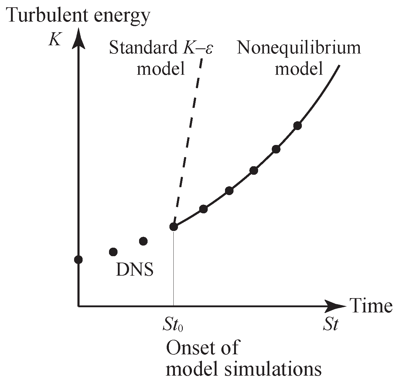
where $C_{\nu }$ is model constant usually taken as $C_{\nu }=0.09$. However, it has long been known that the standard K–$\epsilon$ model with the turbulent viscosity (18) applied to practical flows has some obvious drawbacks. The representative situations where the standard K–$\epsilon$ model fails include the cross-flow configuration with the circumferential or rotating velocity component as well as the axial one, which impinges flow configuration. Another example is the overestimate of the turbulent energy K and its dissipation rate $\epsilon$ in the homogeneous-shear turbulence. The results of the standard K–$\epsilon$ show a tremendously overestimated turbulent energy K as compared with the counterpart in the direct numerical simulations (DNSs) as schematically depicted in Figure 1. Even in one of the simplest flow geometries such as the homogeneous shear, a simple turbulent viscosity model fundamentally fails to reproduce turbulent flow characteristics.

In order to rectify such drawbacks of the standard K–$\epsilon$ model, several improvements to the model have been proposed. A possible improvement of the model is the implementation of the non-equilibrium effect on the basis of a statistical theory of inhomogeneous turbulence. The non-equilibrium effect on turbulent viscosity was investigated with the two-scale direct-interaction approximation (TSDIA) [30,35]. In the framework of the TSDIA, the formal solution of the lowest-order turbulent velocity arising from the large-scale inhomogeneities in space and time is given in terms of the homogeneous isotropic basic field ${\mathbf{u}}_0^{\prime }(\mathbf{k};{\tau }_1)$ and the response function $G^{\prime }(\mathbf{k};\tau ,{\tau }_1)$ as

$$\begin{array}{ccc}{u}_1^{\prime }{}^{\alpha }(\mathbf{k};\tau )\hfill & =& \frac{\partial U^b}{\partial X^a}{\int }_{-\infty }^{\tau }d{\tau }_1{G}^{\prime }{}^{\alpha b}(\mathbf{k};\tau ,{\tau }_1)u_0^{\prime }{}^a(\mathbf{k};{\tau }_1)\hfill \\ & & -{\int }_{-\infty }^{\tau }d{\tau }_1{G}^{\prime }{}^{\alpha a}(\mathbf{k};\tau ,{\tau }_1)\frac{D{u}_0^{\prime }{}^a(\mathbf{k};{\tau }_1)}{DT}\hfill \\ & & +2M^{dab}\left(\mathbf{k}\right)\int \int \delta (\mathbf{k}-\mathbf{p}-\mathbf{q})d\mathbf{p}d\mathbf{q}{\int }_{-\infty }^{\tau }d{\tau }_1{G}^{\prime }{}^{\alpha d}(\mathbf{k};\tau ,{\tau }_1)\frac{q^b}{q^2}{u}_0^{\prime }{}^a(\mathbf{p};{\tau }_1)\frac{\partial u^{\prime }{}_0^c(\mathbf{q};{\tau }_1)}{\partial X^c}\hfill \\ & & \hfill -M^{abcd}\left(\mathbf{k}\right)\int \int \delta (\mathbf{k}-\mathbf{p}-\mathbf{q})d\mathbf{p}d\mathbf{q}{\int }_{-\infty }^{\tau }d{\tau }_1{G}^{\prime }{}^{\alpha d}(\mathbf{k};\tau ,{\tau }_1)\frac{\partial }{\partial X^c}\left(u_0^{\prime }{}^a(\mathbf{p};{\tau }_1)u_0^{\prime }{}^b(\mathbf{q};{\tau }_1)\right).\hfill \end{array}$$

(19)

Here, the second term on the right-hand side related to the Lagrange derivative represents the non-equilibrium properties of the turbulent field along the flow. The turbulent kinetic energy K with the non-equilibrium effect is written as

$$\begin{array}{ccc}\hfill K& =& \langle {\mathbf{u}}^{\prime }{}^2\rangle /2=\frac{1}{2}\int d\mathbf{k}\langle u^{\prime }{}^{\mathsf{\ell }}(\mathbf{k};\tau )u^{\prime }{}^{\mathsf{\ell }}({\mathbf{k}}^{\prime };\tau )\rangle /\delta (\mathbf{k}+{\mathbf{k}}^{\prime })\hfill \\ & =& (\langle u_0^{\prime }{}^{\mathsf{\ell }}{u}_0^{\prime }{}^{\mathsf{\ell }}\rangle +\langle u_0^{\prime }{}^{\mathsf{\ell }}{u}_1^{\prime }{}^{\mathsf{\ell }}\rangle +\langle u_1^{\prime }{}^{\mathsf{\ell }}{u}_0^{\prime }{}^{\mathsf{\ell }}\rangle +\cdots )/2\hfill \\ & =& C_{K1}{\epsilon }^{2/3}{\mathsf{\ell }}_{\mathrm{C}}^{2/3}-C_{K2}{\epsilon }^{-3/2}{\mathsf{\ell }}_{\mathrm{C}}^{4/3}\frac{D\epsilon }{Dt}-C_{K3}{\epsilon }^{1/3}{\mathsf{\ell }}_{\mathrm{C}}^{1/3}\frac{D{\mathsf{\ell }}_{\mathrm{C}}}{Dt},\hfill \end{array}$$

(20)

where ${\mathsf{\ell }}_{\mathrm{C}}$ is the length scale of the largest eddy and $D/Dt(=\partial /\partial t+\mathbf{U}·\mathsf{\nabla })$ is the Lagrange or material derivative along the mean-flow velocity. Here, $C_{Kn}(n$ = 1–3) are the model constants whose magnitudes are related to those of the energy spectrum and the time scale of turbulence (${\sigma }_0$ in (A5) and ${\omega }_0$ in (A6)). A brief derivation of (20) is given in Appendix A.

We solve (20) with respect to ${\mathsf{\ell }}_{\mathrm{C}}$ by an iteration method with the first term of (20) as the starting term:

$$K=C_{K1}{\epsilon }^{2/3}{\mathsf{\ell }}_{\mathrm{C}}^{2/3}.$$

(21)

Then, we have ${\mathsf{\ell }}_{\mathrm{C}}$ as

$${\mathsf{\ell }}_{\mathrm{C}}=C_{\mathsf{\ell }1}{K}^{3/2}{\epsilon }^{-1},$$

(22)

where $C_{\mathsf{\ell }1}$ is the model constant. With (13), this lowest-order expression of the length scale corresponds to the simplest eddy viscosity model (18).

Substituting (18) into (20), we have the first iteration result as

$${\mathsf{\ell }}_{\mathrm{C}}=C_{\mathsf{\ell }1}{K}^{3/2}{\epsilon }^{-1}+C_{\mathsf{\ell }2}{K}^{3/2}{\epsilon }^{-2}\frac{DK}{Dt}-C_{\mathsf{\ell }3}{K}^{5/2}{\epsilon }^{-3}\frac{D\epsilon }{Dt}$$

(23)

($C_{\mathsf{\ell }2}$ and $C_{\mathsf{\ell }3}$ are model constants). The second and third terms of (23) represent the non-equilibrium effect. Equation (23) shows that the length scale of turbulence, as well as the time scale and energy of turbulence, is corrected by the $D/Dt$-related non-equilibrium effect terms. Equation (23) can be approximated as

$${\mathsf{\ell }}_{\mathrm{C}}={\mathsf{\ell }}_{\mathrm{E}}\left(1-C_{\mathrm{N}}^{\prime }\frac{1}{K}\frac{D}{Dt}\frac{K^2}{\epsilon }\right),$$

(24)

where ${\mathsf{\ell }}_{\mathrm{E}}$ is the equilibrium characteristic length defined by

$${\mathsf{\ell }}_{\mathrm{E}}=K^{3/2}/\epsilon ,$$

(25)

and $C_{\mathrm{N}}^{\prime }$ is the non-equilibrium-effect-related coefficient. Depending on the streamwise development of the turbulent energy K and its dissipation rate $\epsilon$, the length scale of turbulence changes as compared to the equilibrium cases. At the same time, the time scale of the non-equilibrium turbulence may be expressed as

$${\tau }_{\mathrm{NS}}=\frac{{\mathsf{\ell }}_{\mathrm{NS}}}{K^{1/2}}\simeq C_{\mathrm{S}}^{-3/2}\frac{K}{\epsilon }\left(1-C_{\mathrm{N}}^{\prime }\frac{1}{K}\frac{D}{Dt}\frac{K^2}{\epsilon }\right).$$

(26)

This indicates that the effective time scale may change depending on the $D/Dt$ effect.

The non-equilibrium turbulent viscosity ${\nu }_{\mathrm{T}}$ can be expressed as

$${\nu }_{\mathrm{T}}=C_{\nu }\frac{K^2}{\epsilon }-C_{\nu K}\frac{K^2}{{\epsilon }^2}\frac{DK}{Dt}+C_{\nu \epsilon }\frac{K^3}{{\epsilon }^3}\frac{D\epsilon }{Dt},$$

(27)

where $C_{\nu }$, $C_{\nu K}$ and $C_{\nu \epsilon }$ are the model constants whose values can be evaluated from theoretical analyses. Equation (27) is rewritten as

$${\nu }_{\mathrm{T}}=C_{\nu }\frac{K^2}{\epsilon }\left[1-\left(C_{\mathrm{N}K}\frac{1}{\epsilon }\frac{DK}{Dt}-C_{\mathrm{N}\epsilon }\frac{K}{{\epsilon }^2}\frac{D\epsilon }{Dt}\right)\right],$$

(28)

or approximately

$${\nu }_{\mathrm{T}}=C_{\nu }\frac{K^2}{\epsilon }\left(1-C_{\mathrm{N}}\frac{1}{K}\frac{D}{Dt}\frac{K^2}{\epsilon }\right)$$

(29)

($C_{\mathrm{N}K}$, $C_{\mathrm{N}\epsilon }$ and $C_{\mathrm{N}}$: model constants). Here, we should note that this non-equilibrium effect does not necessarily require compressibility. This effect shows up even in incompressible cases.

In practical situations wherein turbulent flows are simulated, a large positive $D/Dt$ term may occur locally; in such a case, (29) may lead to a physically undesirable negative turbulent viscosity. In order to alleviate such an unphysical model result to enhance the applicability of the model expression, we use a simple Padé approximation to (29) and have

$${\nu }_{\mathrm{T}}=\left\{\begin{array}{ccc}\hfill {\nu }_{\mathrm{TE}}{\left(1+C_{\mathrm{N}}\frac{1}{K}\frac{D}{Dt}\frac{K^2}{\epsilon }\right)}^{-1}\hfill & \hfill \mathrm{for}\hfill & \hfill \frac{D}{Dt}\frac{K^2}{\epsilon }>0,\hfill \\ \hfill {\nu }_{\mathrm{TE}}\left(1-C_{\mathrm{N}}\frac{1}{K}\frac{D}{Dt}\frac{K^2}{\epsilon }\right)\hfill & \hfill \mathrm{for}\hfill & \hfill \frac{D}{Dt}\frac{K^2}{\epsilon }<0,\hfill \end{array}\right.$$

(30)

where the equilibrium eddy viscosity ${\nu }_{\mathrm{TE}}$ is defined in the same form as (18) by

$${\nu }_{\mathrm{TE}}=C_{\nu }\frac{K^2}{\epsilon }.$$

(31)

Equation (30) indicates that, depending on the sign of the Lagrangian or material derivative $(D/Dt)(K^2/\epsilon )$, the turbulent viscosity is effectively decreased or increased by the non-equilibrium effect. In the case of $(D/Dt)(K^2/\epsilon )>0$, ${\nu }_{\mathrm{T}}$ is decreased, while in the case of $(D/Dt)(K^2/\epsilon )<0$, ${\nu }_{\mathrm{T}}$ is increased. This implies that, in this case, the non-equilibrium effect works in the direction to stabilize the deviation from the equilibrium state (return to equilibrium).

The non-equilibrium model expression for the eddy viscosity (30) has been applied to the homogeneous-shear turbulence, where the standard K–$\epsilon$ model with the conventional eddy viscosity (31) leads to an overestimated turbulent energy K and its dissipation rate $\epsilon$ as compared to the DNS results (Figure 1). It was reported that the non-equilibrium model (30) with $C_{\mathrm{N}}=0.8$ leads to the results consistent with the DNS ones [6]. In this sense, the validity of the non-equilibrium effects in turbulent mixing has been already confirmed in a simple geometrical flow.

4. Non-Equilibrium Effects in Jet and Plume Experiments

As was referred to in Section 1, in the buoyancy-dominated turbulent flows, the turbulent convection is characterized by large-scale plumes. As this consequence, the turbulent fluxes are deviated from the usual gradient-transport approximation. It has been recognized that entrainment dominates the evolution of buoyant plumes [11]. As was shown in a previous study of a supernova convection [21], global turbulence models introducing the entrainment parameters provide the best results for describing the evolution of buoyant plumes. However, such models highly depend on the geometrical configurations of the simulation, and are difficult to apply to a general 3D situation. In this sense, it is preferable to develop a local model without resorting to global parameters, provided that the local model works well enough for reproducing the basic behavior of the convection turbulence with plumes. In order to validate the model, here we consider turbulent flows with much simpler geometrical configurations, namely jets and plumes, utilizing recent experimental results.

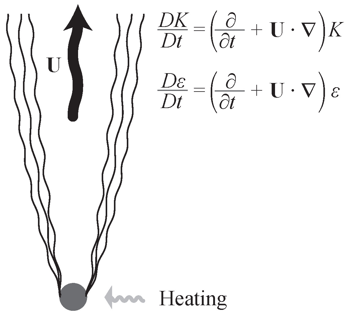
The non-equilibrium effect may help develop such a local model. In the presence of a plume, we can expect that the turbulence properties vary in the plume-flow direction. The non-equilibrium effect associated with the plume motion can be incorporated through the variation in the turbulent energy K and its dissipation rate $\epsilon$ along the plume motion in terms of the Lagrangian or advective derivatives, $DK/Dt=\left[\right(\partial /\partial t)+\mathbf{U}·\mathsf{\nabla }]K$ and $D\epsilon /Dt=\left[\right(\partial /\partial t)+\mathbf{U}·\mathsf{\nabla }]\epsilon$ (Figure 2). The effect of non-equilibrium turbulence can be implemented into the model of turbulent viscosity as (30) with the equilibrium turbulent viscosity given by (31).

Recently, a series of detailed experimental studies of the budgets of turbulent energy, Reynolds stresses and dissipation rate has been performed in single- and multi-phase jets/plumes, including a turbulent round jet discharged into an initially stationary ambient [27], a buoyant multi-phase bubble plume [28], a negatively buoyant multi-phase particle plume [25] and a variable density round jet with co-flow [26].

4.1. Round Jets

Using a set of stereoscopic particle image velocimetry (SPIV) measurements of a turbulent round water jet, the budget of the turbulent energy equation was investigated in Lai and Socolofsky [27]. In this experiment, it was reported that the magnitudes of the normal Reynolds stresses $R^{ii}$ decreased by 30 % over $27\le x/D\le 37$ in the downstream direction (D: exit diameter of the jet nozzle). In particular, the streamwise variation of the axial velocity fluctuation $\langle {\left(u^{\prime }{}^x\right)}^2\rangle /\sqrt{\epsilon }$ at the jet centerline shows a decreasing tendency at the major region of the axial locations $31\le x/D\le 37$ (

Table 1. Streamwise variation of normalized turbulent intensities, turbulent energy and turbulent axial velocity fluctuation normalized by the square root of the dissipation rate at the jet centerline. $x/D$: jet streamwise length, D: jet nozzle exit diameter ($D=11\mathrm{mm}$), $U_{\mathrm{c}}$: centerline jet velocity ($U_{\mathrm{c}}=50\mathrm{mm}{\mathrm{s}}^{-1}$). Data are taken from Figures 7 and 8 of Lai and Socolofsky [27].

$\mathit{x}/\mathit{D}$	$\sqrt{\langle {\left({\mathit{u}}^{\prime }{}^{\mathit{x}}\right)}^2\rangle }/{\mathit{U}}_{\mathbf{c}}$	$\sqrt{\langle {\left({\mathit{u}}^{\prime }{}^{\mathit{y}}\right)}^2\rangle }/{\mathit{U}}_{\mathbf{c}}$	$\sqrt{\langle {\left({\mathit{u}}^{\prime }{}^{\mathit{z}}\right)}^2\rangle }/{\mathit{U}}_{\mathbf{c}}$	$\mathit{K}/{\mathit{U}}_{\mathbf{c}}^2$	$\langle {\left({\mathit{u}}^{\prime }{}^{\mathit{x}}\right)}^2\rangle /\sqrt{{\mathit{\epsilon }}_{\mathbf{iso}}}$
31	0.26	0.20	0.19	0.1437	$3.25\times {10}^{-2}$
37	0.26	0.20	0.19	0.1437	$2.65\times {10}^{-2}$
					(−20%)

). Although in Lai and Socolofsky [27], these experimental results are argued in the context of the approximate achievement of the self-preserving state in the jet [36]; this decrease tendency may be interpreted as a deviation from the self-preserving state due to the non-equilibrium effect. Since the magnitude of axial velocity fluctuation $\sqrt{\langle {\left(u^{\prime }{}^x\right)}^2\rangle }$ is similar to and just slightly larger than the horizontal counterparts of the velocity fluctuations, $\sqrt{\langle {\left(u^{\prime }{}^y\right)}^2\rangle }$ and $\sqrt{\langle {\left(u^{\prime }{}^z\right)}^2\rangle }$, and since the energy dissipation rate $\epsilon$ is well represented by that of the isotropic turbulence, ${\epsilon }_{\mathrm{iso}}$, the evolution of squared axial velocity fluctuation, $\langle {\left(u^{\prime }{}^x\right)}^2\rangle /\sqrt{{\epsilon }_{\mathrm{iso}}}$, provides a reasonable surrogate for the basic behavior of $K^2/\epsilon$:

$$\frac{K^2}{\epsilon }\propto {\left[\frac{\langle {\left(u^{\prime }{}^x\right)}^2\rangle }{\sqrt{{\epsilon }_{\mathrm{iso}}}}\right]}^2.$$

(32)

The decrease in $\langle {\left(u^{\prime }{}^x\right)}^2\rangle /\sqrt{{\epsilon }_{\mathrm{iso}}}$ in the downstream direction indicates that the sign of the non-equilibrium effect term is negative as

$$\frac{D}{Dt}\frac{K^2}{\epsilon }<0\left(\mathrm{in}\mathrm{turbulent}\mathrm{round}\mathrm{jets}\right).$$

(33)

It follows from (30) that the turbulent viscosity is enhanced by the non-equilibrium effect as

$${\nu }_{\mathrm{NE}}={\nu }_{\mathrm{E}}\left(1-C_{\mathrm{N}}\frac{1}{K}\frac{D}{Dt}\frac{K^2}{\epsilon }\right)>{\nu }_{\mathrm{E}}.$$

(34)

In order to evaluate the non-equilibrium effect, we introduced the non-equilibrium correction factor $\mathsf{\Lambda }$ by

$$\mathsf{\Lambda }=C_{\mathrm{N}}\frac{1}{K}\frac{D}{Dt}\frac{K^2}{\epsilon },$$

(35)

where $C_{\mathrm{N}}$ is the model constant estimated as the order of unity ($C_{\mathrm{N}}=0.8$) through applications to the homogeneous-shear flow turbulence [6]. This factor is approximated in terms of the Lagrangian derivative as

$$\mathsf{\Lambda }\simeq C_{\mathrm{N}}\frac{1}{K}(\mathbf{U}·\mathsf{\nabla })\frac{K^2}{\epsilon }.$$

(36)

Using the data of Lai and Socolofsky [27], $\mathsf{\Lambda }$ is estimated as

$$\begin{array}{c}\hfill \mathsf{\Lambda }\simeq C_{\mathrm{N}}{\left(\frac{U_{\mathrm{c}}}{\sqrt{\langle {\left(u^{\prime }{}^x\right)}^2\rangle }}\right)}^2\frac{1}{U_{\mathrm{c}}}\frac{\Delta \left\{{[\langle {\left(u^{\prime }{}^x\right)}^2\rangle /\sqrt{\langle {\epsilon }_{\mathrm{iso}}\rangle }]}^2\right\}}{D\Delta (x/D)}\simeq 1.7\end{array}$$

(37)

with $C_{\mathrm{N}}=1$ (Table 1). Here, $\Delta \left\{{[\langle {\left(u^x\right)}^2\rangle /\sqrt{\langle {\epsilon }_{\mathrm{iso}}\rangle }]}^2\right\}$ in the nominator and $\Delta (x/D)$ in the denominator are the increments in ${[\langle {\left(u^x\right)}^2\rangle /\sqrt{\langle {\epsilon }_{\mathrm{iso}}\rangle }]}^2$ and $x/D$ along the jet streamwise direction.

In Lai and Socolofsky [27], the budgets of the turbulent energy and dissipation rate equations were also investigated. Using the balance in the budgets, the coefficients of each term of the K–$\epsilon$ model were examined. They suggested the befitting directions for the change in model coefficients. The eddy viscosity constant $C_{\nu }$ was increased from the standard value of $C_{\nu }=0.09$ to 0.09–0.27, whereas a reduction of $C_{\nu }$ to $0.07$ is suggested from the matching for the jet spreading rate. This implies that it is inadequate to use a constant model coefficient $C_{\nu }$ for the turbulent viscosity. The enhancement of eddy viscosity due to the non-equilibrium effect is basically in the correct direction to the evaluation of $C_{\nu }$, and the estimated value of $\mathsf{\Lambda }$ (37) is consistent with the suggested change of $C_{\nu }$. The degree of enhancement/suppression should be determined by the non-equilibrium property of the turbulence, which depends on the spatial location.

4.2. Buoyant Bubble Plumes

In Lai and Socolofsky [28], the turbulent energy budgets in bubble plume were experimentally investigated. There, the turbulent energy evolution was measured both in the adjustment phase of the plume dependent on the source conditions (source size and geometry) and in the asymptotic phase independent of the source condition.

These experimental results show that, in the asymptotic phase (Case A), the turbulent energy K, its dissipation rate $\epsilon$ and $K^2/\epsilon$ in the plume core region ($r\le b_g$) decrease in the axial or downstream direction along the plume velocity, while in the adjustment phase (Case B) K, $\epsilon$ and $K^2/\epsilon$ increase (

Table 2. Evolutions of turbulent energy and its dissipation rate along the plume flow. Case A is the asymptotic phase and Case B is the adjustment phase. $z/D$: vertical streamwise height; D: dynamic length scale ($D=6.8\mathrm{cm}$ for Case A and $D=20.4\mathrm{cm}$ for Case B); $W_{\mathrm{c}}$: plume centerline velocity; and $b_g$: Gaussian plume radius. Data are taken from Figures 20 and 25 of Lai and Socolofsky [28].

Case A (Asymptotic Phase)
$z/D$	$W_{\mathrm{c}}$ ($\mathrm{cm}{\mathrm{s}}^{-1}$)	$b_g$	$K/W_{\mathrm{c}}^2$	$(\epsilon /W_{\mathrm{c}}^3)b_g\times {10}^3$	K (${\mathrm{cm}}^2{\mathrm{s}}^{-2}$)	$\epsilon$ (${\mathrm{cm}}^2{\mathrm{s}}^{-3}$)	$K^2/\epsilon$ (${\mathrm{cm}}^2{\mathrm{s}}^{-1}$)
6.6	20.64	5.46	0.135	0.04	57.51	64.42	51.34
11.0	17.90	8.00	0.165	0.086	52.87	61.65	45.34
					(−8.1%)	(−4.3%)	(−11.7%)
Case B (Adjustment Phase)
$z/D$	$W_{\mathrm{c}}$ ($\mathrm{cm}{\mathrm{s}}^{-1}$)	$b_g$	$K/W_{\mathrm{c}}^2$	$(\epsilon /W_{\mathrm{c}}^3)b_g\times {10}^3$	K (${\mathrm{cm}}^2{\mathrm{s}}^{-2}$)	$\epsilon$ (${\mathrm{cm}}^2{\mathrm{s}}^{-3}$)	$K^2/\epsilon$ (${\mathrm{cm}}^2{\mathrm{s}}^{-1}$)
2.19	28.50	5.27	0.15	0.035	121.84	153.74	96.56
3.66	25.14	8.53	0.225	0.0896	142.20	165.78	121.97
					(+16.7%)	(+7.8%)	(+26.3%)

). However, the relative variation in the turbulent kinetic energy at the downstream to the upstream is much higher in the adjustment phase (Case B) than in the asymptotic phase (Case A). This means that the turbulent energy inhomogeneity along the plume flow, which may lead to the non-equilibrium effect is more prominent in the adjustment phase than in the asymptotic phase. This is natural since the non-equilibrium property is expected to be much higher in the adjustment phase than in the asymptotic phase. In the adjustment phase, the Lagrangian derivative of $K^2/\epsilon$ is positive as

$$\frac{D}{Dt}\frac{K^2}{\epsilon }>0\left(\mathrm{in}\mathrm{the}\mathrm{adjustment}\mathrm{phase}\mathrm{of}\mathrm{buoyant}\mathrm{bubble}\mathrm{plume}\right).$$

(38)

In this case, from (30)

$${\nu }_{\mathrm{NE}}={\nu }_{\mathrm{E}}{\left(1+\mathsf{\Lambda }\right)}^{-1}<{\nu }_{\mathrm{E}}\left(\mathrm{in}\mathrm{the}\mathrm{adjustment}\mathrm{phase}\mathrm{of}\mathrm{buoyant}\mathrm{bubble}\mathrm{plume}\right).$$

(39)

In the experiment of Lai and Socolofsky [28], $\mathsf{\Lambda }$ is estimated as

$$\begin{array}{ccc}\hfill \mathsf{\Lambda }& \simeq & \hfill C_{\mathrm{N}}\frac{1}{K}{W}_{\mathrm{c}}\frac{\Delta (K^2/\epsilon )}{D\Delta (z/D)}\simeq 0.20\hfill \end{array}$$

(40)

with $C_{\mathrm{N}}=1$ (Table 2). Here, $\Delta (K^2/\epsilon )$ and $\Delta (z/D)$ are the increments of $K^2/\epsilon$ and $z/D$ along the vertical streamwise height, respectively. This suggests that due to the non-equilibrium effect, the turbulent mixing in the buoyant bubble plumes is expected to be suppressed by a few 10% as compared to the standard equilibrium turbulent transport.

4.3. Variable Density Jets

There are several studies on the buoyancy-driven variable density turbulence with jets and plumes [26,37]. In recent experiments by Charonko and Prestridge [26], variable density effects in turbulent round jets with co-flow at high- and low-density ratios are experimentally investigated. There, the axial and radial mixing mechanisms of jet are compared between the cases with low and high variable density contrast. It was confirmed that the Reynolds stress is suppressed by the turbulent mass flux in the increased variable density case. It was also reported that the radial transport of momentum and the energy cascade down to small scales are significantly suppressed in the variable density case. These suppressions mostly take place in locations where the density fluctuation is large.

At the upstream region ($x_1/d_0<16.3$, $x_1$: axial location; $d_0$: inner diameter), the turbulent energy—regardless of both whether averaging is mass-weighted or the Reynolds and whether turbulent energy is normalized by excess momentum or the initial kinetic energy of the mean flow—develops with a downstream distance along the centerline as

$$\frac{DK}{Dt}>0\left(\mathrm{at}\mathrm{upstream}\mathrm{region}\mathrm{of}\mathrm{variable}\mathrm{density}\mathrm{jets}\right).$$

(41)

This increase in turbulent energy along the mean flow takes place in both the small- and large-density variation cases. Since the evolution of the dissipation rate $\epsilon$ with the axial distance is not explicitly presented in Charonko and Prestridge [26], that of $K^2/\epsilon$ cannot be accurately evaluated. However, the analysis of several flows later in Section 5.1 implies that the trend of the $K^2/\epsilon$ evolution along the mean flow or the sign of $K^2/\epsilon$ can be surmised from the evolution of K itself. From the non-equilibrium effect $D(K^2/\epsilon )/Dt[\sim (K/\epsilon )DK/Dt]$ in (30), we see that the turbulent transport is suppressed at the upstream region.

At the same time, Charonko and Prestridge [26] showed that the variable density effects decrease both the peak and asymptotic values of turbulent energy. By considering the budget in the evolution equation of turbulent energy, they suggested that in the high variable density case, the density fluctuation contributes to the suppression of energy transfer into small-scale fluctuations and preserving the mean-flow structures further downstream. These features can be well understood from the viewpoint of a density-variance effect; the presence of density variance $K_{\rho }(=\langle {\rho }^{\prime }{}^2\rangle )$ leads to the suppression of turbulent transport as in (30). Charonko and Prestridge [26] concluded that the variable density effect must be modeled to accurately capture dynamical mixing in jets and other variable density flow phenomena. The combination of the non-equilibrium and density-variance effects proposed in the present work is a candidate for modeling the variable density effect in these flows.

5. Plumes in Stellar Convection Zone

In the previous section, we argued the non-equilibrium effect associated with a single plume and jet. In modeling such a situation, the velocity of the single plume/jet is treated as the local mean velocity, and the non-equilibrium effect associated with the mean velocity can be captured by the Lagrangian or advective derivative $D/Dt=\partial /\partial t+\mathbf{U}·\mathsf{\nabla }$ [$\mathbf{U}(\equiv \langle \mathbf{u}\rangle )$: mean velocity]. However, in the practical application of the turbulence model to geo/astrophysical flow phenomena, we often encounter situations where the effect of numerous plumes and jets on the global or averaged flow dynamics must be properly evaluated.

One example is the turbulent transport in the stellar convection zone. In some flow configurations, such as in the convective motion in a closed domain, the mean velocity formulated with a simple ensemble average or averaging in the statistically homogeneous plane is very small because of the statistical cancellations due to symmetry. Furthermore, such an averaged quantity cannot capture localized flow structures such as plumes. Because of the small mean flow ($\langle \mathbf{u}\rangle \equiv \mathbf{U}\simeq 0$), the non-equilibrium effect represented by the mean flow advection, $(\mathbf{U}·\mathsf{\nabla })K^2/\epsilon$ in $DK/Dt$, is not suitable for capturing the plume effects. With a simple ensemble or space-averaging procedure, the direct impact due to the non-equilibrium effect might be negligible. However, the presence of grid-scale (GS) or large-eddy velocity component suggests that the counterpart of the non-equilibrium effect at GS may arise as a result of the alternation of the subgrid-scale (SGS) turbulent transport.

5.1. Non-Equilibrium Effect in the Stellar Convection

Recently, in the context of the stellar convection, the non-equilibrium effects associated with the convective plume motion were investigated in the framework of double averaging [29]. For the purpose of exploring the non-equilibrium effect associated with the plumes, fluid dynamics in the stellar convection zone was investigated with the aid of direct numerical simulations (DNSs). In the setup of the simulations, the diving plumes are driven by the cooling layer at the upper surface of the stellar convection zone. Because of the cooling, the surface layer is convectively unstable.

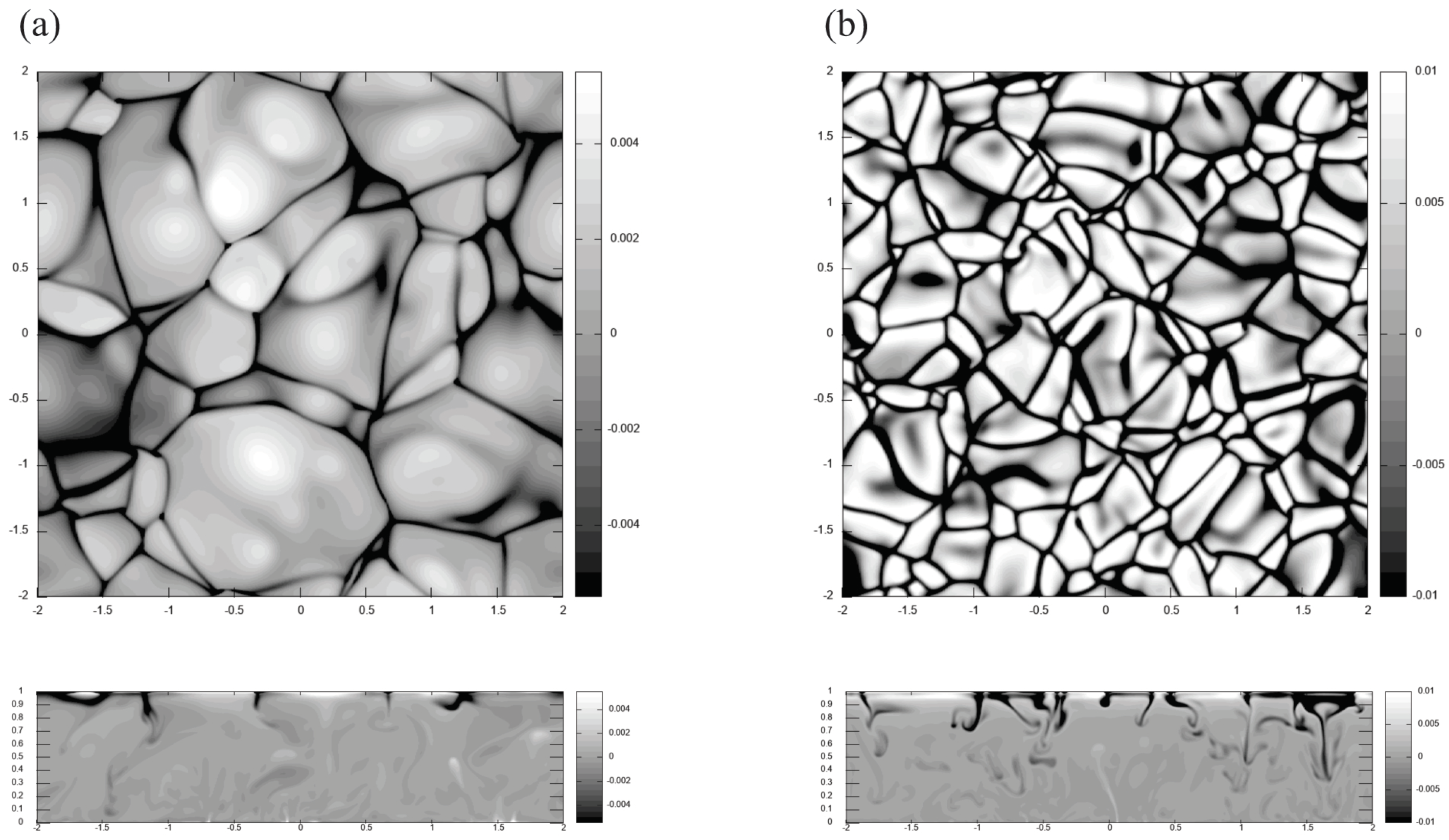
In the non-locally driven convection case, there exist a lot of downward plumes in the shallow region of the convection zone as in the lower plot of Figure 3b.

In order to capture the dynamics of plume motion, the time–space double-averaging procedure was adopted there. A field quantity f is divided into

$$f=\stackrel{\overline{f}}{\overbrace{\langle \overline{f}\rangle +\underset{\begin{array}{c}\overline{f}-\langle \overline{f}\rangle \\ \mathrm{coherent}\\ \mathrm{fluctuation}\end{array}}{\underbrace{\tilde{f}}}}}+\underset{\begin{array}{c}f-\overline{f}\\ \mathrm{incoherent}\\ \mathrm{fluctuation}\end{array}}{\underbrace{f^{″}}},$$

(42)

where $\overline{f}$ denotes the time average, $\langle f\rangle$ denotes the space or ensemble average and $\tilde{f}(=\overline{f}-\langle \overline{f}\rangle )$ denotes the residual of the temporal average subtracted by the ensemble average part. This part may be called the dispersion or coherent fluctuation of f, $f^{″}(=f-\overline{f})$, the fluctuation around the time average $\overline{f}$. As for the time averaging, the resolved part of a quantity f, $\overline{f}$, is defined by the relation

$$\overline{f}(\mathbf{x};t)=\int f(\mathbf{x};s)G(t-s)ds$$

(43)

with the simplest top-hat time filter function $G(t-s)$ defined by

$$G(t-s)=\left\{\begin{array}{cc}1/T\hfill & \left(\right|t-s|\le T/2),\hfill \\ 0\hfill & \left(\mathrm{otherwise}\right).\hfill \end{array}\right.$$

(44)

Here, T is the averaging time window, which should be put in the range:

$$\tau \ll T\ll \Xi ,$$

(45)

where $\tau$ is the eddy turnover time of turbulence and $\Xi$ is the time scale of the mean-field evolution.

In this formalism, the fluctuation around the space or ensemble average, $f^{\prime }$, is divided into the coherent and incoherent parts as

$$f^{\prime }=\tilde{f}+f^{\prime \prime }.$$

(46)

With this double-averaging procedure, the time-averaged velocity $\overline{\mathbf{u}}$ is divided into the space-averaged velocity $\langle \overline{\mathbf{u}}\rangle$ and the dispersion velocity $\tilde{\mathbf{u}}$ as

$$\overline{\mathbf{u}}=\langle \overline{\mathbf{u}}\rangle +\tilde{\mathbf{u}}.$$

(47)

The non-equilibrium effect along the plume motion is represented by the factor

$${\tilde{\mathsf{\Lambda }}}_{\mathrm{D}}=〈(\tilde{\mathbf{u}}·\mathsf{\nabla })\overline{{\mathbf{u}}^{\prime }{}^2}〉.$$

(48)

This means that, if the turbulent energy is inhomogeneous along the plume motion $\tilde{\mathbf{u}}$, the turbulent fluxes are enhanced or suppressed depending on the sign of ${\tilde{\mathsf{\Lambda }}}_{\mathrm{D}}$.

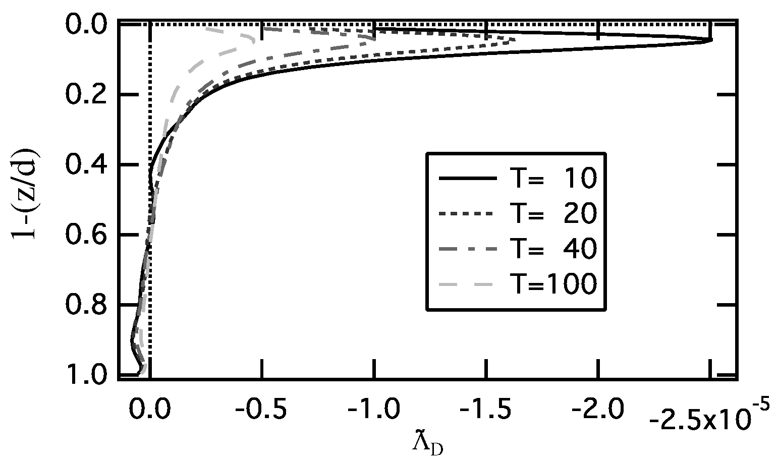
Realizations of the non-equilibrium factor ${\tilde{\mathsf{\Lambda }}}_{\mathrm{D}}=\langle (\tilde{\mathbf{u}}·\mathsf{\nabla })\overline{{\mathbf{u}}^{\prime }{}^2}\rangle$ in the stellar convection simulations are plotted in Figure 4. In this case, statistically, the plume velocity is in the downward direction (${\tilde{u}}^z<0$) while the turbulent energy $\overline{{\mathbf{u}}^{\prime }{}^2}$ decreases in the downward direction ($\partial \overline{{\mathbf{u}}^{\prime }{}^2}/\partial z>0$). As a result, the non-equilibrium factor ${\tilde{\mathsf{\Lambda }}}_{\mathrm{D}}$ is statistically negative as

$${\tilde{\mathsf{\Lambda }}}_{\mathrm{D}}=〈(\tilde{\mathbf{u}}·\mathsf{\nabla })\overline{{\mathbf{u}}^{\prime }{}^2}〉=〈{\tilde{u}}^z\frac{\partial \overline{{\mathbf{u}}^{\prime }{}^2}}{\partial z}〉<0.$$

(49)

The spatial distribution of ${\tilde{\mathsf{\Lambda }}}_{\mathrm{D}}$ is concentrated in the region near the surface where the diving plume structures are prominently observed. The magnitude of ${\tilde{\mathsf{\Lambda }}}_{\mathrm{D}}$ shows a much larger value in the case with the smaller averaging time window T defined in (44). This clearly shows that the non-equilibrium effect associated with the plume motion can be captured by the Lagrangian derivative of the turbulent energy along the plume motion.

In the framework of the time–space-averaging procedure, the non-equilibrium effect is incorporated into the turbulent internal-energy flux. On the basis of the eddy viscosity expression (30) in the usual ensemble averaging procedure, the turbulent internal-energy diffusivity ${\kappa }_{\mathrm{T}}$ with the non-equilibrium effect in the time–space-averaging procedure may be formulated as

$${\kappa }_{\mathrm{T}}={\kappa }_{\mathrm{TE}}\left(1-\tilde{C}{\langle \overline{\rho }\rangle }^{-1/3}{\tilde{\mathsf{\Lambda }}}_{\mathrm{D}}\right),$$

(50)

where ${\kappa }_{\mathrm{TE}}$ is the equilibrium turbulent internal-energy diffusivity, $\langle \overline{\rho }\rangle$ is the horizontally averaged density and $\tilde{C}$ is the model constant. The mean density dependence ${\langle \overline{\rho }\rangle }^{-1/3}$ in (50) is obtained from the argument that the coherent dissipation rate $\tilde{\epsilon }$ is proportional to the cubic root of the buoyancy flux associated with a plume. See Section 6.3 and Appendix C of Yokoi, Masada and Takiwaki [29] for the detailed arguments on this dependence.

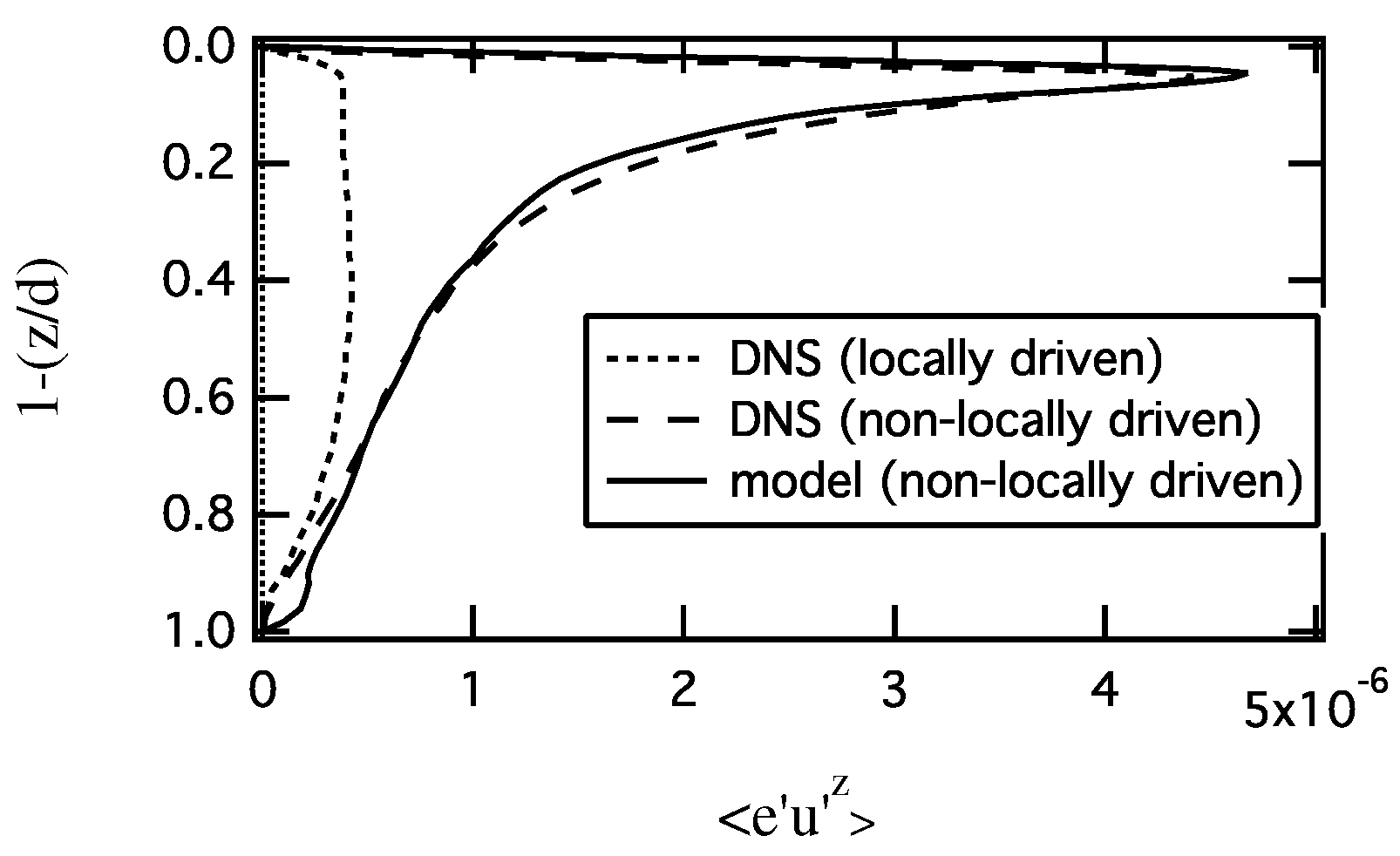
The turbulent internal-energy flux $\langle e^{\prime }{u}^{\prime }{}^z\rangle$ obtained from the DNSs in the locally and non-locally driven convection cases, which, respectively, correspond to (a) and (b) of Figure 3, are plotted in Figure 5. We see from the figure that the spatial profiles of these two cases are fairly different. First, the magnitude of $\langle e^{\prime }{u}^{\prime }{}^z\rangle$ is much larger in the non-locally driven convection case. At the same time, turbulent transport is significantly localized near the surface region in the non-locally driven case. These prominent properties of turbulent transport in the non-locally driven convection cannot be properly reproduced by the usual gradient-diffusion model with the mixing-length theory.

The spatial distribution of $\langle e^{\prime }{u}^{\prime }{}^z\rangle$ calculated by the model with the non-equilibrium effect (50):

$$\langle e^{\prime }{u}^{\prime }{}^z\rangle =-{\kappa }_{\mathrm{T}}\mathsf{\nabla }E$$

(51)

which is also plotted in Figure 5 (E: mean internal energy). The comparison with the DNS results shows that the spatial distribution of $\langle e^{\prime }{u}^{\prime }{}^z\rangle$ in the non-locally driven convection is well reproduced by the present model with the non-equilibrium effect.

5.2. Interaction between Coherent and Incoherent Fluctuations

In this double-averaging formulation, the fluctuation around the space or ensemble average, $f^{\prime }$, is divided into the coherent and incoherent components as $f^{\prime }=\tilde{f}+f^{″}$. These two components are not independent but interact with each other. For instance, let us consider the Reynolds stress in the time–space double-averaging procedure. The evolutions of the Reynolds stress of the coherent velocity fluctuation, $\langle \overline{\tilde{\mathbf{u}}\tilde{\mathbf{u}}}\rangle$, are subject to

$$\left(\frac{\partial }{\partial t}+\langle \overline{\mathbf{u}}\rangle ·\mathsf{\nabla }\right)\langle \overline{{\tilde{u}}^i{\tilde{u}}^j}\rangle ={\tilde{P}}^{ij}+{\tilde{\mathsf{\Pi }}}^{ij}-{\tilde{\epsilon }}^{ij}+\frac{\partial {\tilde{T}}^{ij\mathsf{\ell }}}{\partial x^{\mathsf{\ell }}}+{\tilde{\mathcal{P}}}^{ij},$$

(52)

where $\tilde{\mathbf{P}}(=\left\{{\tilde{P}}^{ij}\right\})$, $\tilde{\mathsf{\Pi }}(=\left\{{\tilde{\mathsf{\Pi }}}^{ij}\right\})$, $\tilde{\mathbf{\epsilon }}(=\left\{{\tilde{\epsilon }}^{ij}\right\})$ and $\mathsf{\nabla }·\tilde{\mathbf{T}}(=\left\{\partial {\tilde{T}}^{ij\mathsf{\ell }}/\partial x^{\mathsf{\ell }}\right\})$ are the production, re-distribution, dissipation and the transport rates of the coherent components, respectively. They are defined as

$${\tilde{P}}^{ij}=-\langle {\tilde{u}}^j{\tilde{u}}^{\mathsf{\ell }}\rangle \frac{\partial {\langle u\rangle }^i}{\partial x^{\mathsf{\ell }}}-\langle {\tilde{u}}^i{\tilde{u}}^{\mathsf{\ell }}\rangle \frac{\partial {\langle u\rangle }^j}{\partial x^{\mathsf{\ell }}},$$

(53)

$${\tilde{\mathsf{\Pi }}}^{ij}=-\frac{1}{{\rho }_0}〈\tilde{p}\left(\frac{\partial {\tilde{u}}^i}{\partial x^j}+\frac{\partial {\tilde{u}}^j}{\partial x^i}\right)〉,$$

(54)

$${\tilde{\epsilon }}^{ij}-2\nu 〈\frac{\partial {\tilde{u}}^i}{\partial x^{\mathsf{\ell }}}\frac{\partial {\tilde{u}}^j}{\partial x^{\mathsf{\ell }}}〉,$$

(55)

$$\frac{\partial {\tilde{T}}^{ij\mathsf{\ell }}}{\partial x^{\mathsf{\ell }}}=+\frac{\partial }{\partial x^{\mathsf{\ell }}}\left(-〈{\tilde{u}}^{\mathsf{\ell }}{\tilde{u}}^i{\tilde{u}}^j〉+\langle \tilde{p}{\tilde{u}}^i\rangle {\delta }^{\mathsf{\ell }j}+\langle \tilde{p}{\tilde{u}}^j\rangle {\delta }^{\mathsf{\ell }i}+\nu \frac{\partial }{\partial x^{\mathsf{\ell }}}\langle {\tilde{u}}^i{\tilde{u}}^j\rangle \right).$$

(56)

On the other hand, the evolution of the Reynolds stress of the incoherent velocity fluctuation, $\langle \overline{{\mathbf{u}}^{″}{\mathbf{u}}^{″}}\rangle$, is subject to

$$\left(\frac{\partial }{\partial t}+\langle \overline{\mathbf{u}}\rangle ·\mathsf{\nabla }\right)\langle \overline{u^{″}{}^i{u}^{″}{}^j}\rangle =P^{″}{}^{ij}+{\mathsf{\Pi }}^{″}{}^{ij}-{\epsilon }^{″}{}^{ij}+\frac{\partial T^{″}{}^{ij\mathsf{\ell }}}{\partial x^{\mathsf{\ell }}}+{\mathcal{P}}^{″}{}^{ij},$$

(57)

where ${\mathbf{P}}^{″}(=\left\{P^{″}{}^{ij}\right\})$, ${\mathsf{\Pi }}^{″}(=\left\{{{\mathsf{\Pi }}^{″}}^{ij}\right\})$, ${\mathbf{\epsilon }}^{″}(=\left\{{{\epsilon }^{″}}^{ij}\right\})$ and $\mathsf{\nabla }·{\mathbf{T}}^{″}(=\left\{\partial {T^{″}}^{ij\mathsf{\ell }}/\partial x^{\mathsf{\ell }}\right\})$ are defined as

$$P^{″}{}^{ij}=-\langle u^{″}{}^j{u}^{″}{}^{\mathsf{\ell }}\rangle \frac{\partial {\langle u\rangle }^i}{\partial x^{\mathsf{\ell }}}-\langle u^{″}{}^i{u}^{″}{}^{\mathsf{\ell }}\rangle \frac{\partial {\langle u\rangle }^j}{\partial x^{\mathsf{\ell }}},$$

(58)

$${\mathsf{\Pi }}^{″}{}^{ij}=-\frac{1}{{\rho }_0}〈p^{″}\left(\frac{\partial u^{″}{}^i}{\partial x^j}+\frac{\partial u^{″}{}^j}{\partial x^i}\right)〉-2\nu 〈\frac{\partial u^{″}{}^i}{\partial x^{\mathsf{\ell }}}\frac{\partial u^{″}{}^j}{\partial x^{\mathsf{\ell }}}〉,$$

(59)

$${\epsilon }^{″}{}^{ij}=-2\nu 〈\frac{\partial u^{″}{}^i}{\partial x^{\mathsf{\ell }}}\frac{\partial u^{″}{}^j}{\partial x^{\mathsf{\ell }}}〉,$$

(60)

$$\frac{\partial T^{″}{}^{ij\mathsf{\ell }}}{\partial x^{\mathsf{\ell }}}=+\frac{\partial }{\partial x^{\mathsf{\ell }}}\left(-〈u^{″}{}^{\mathsf{\ell }}{u}^{″}{}^i{u}^{″}{}^j〉+\langle p^{″}{u}^{″}{}^i\rangle {\delta }^{\mathsf{\ell }j}+\langle p^{″}{u}^{″}{}^j\rangle {\delta }^{\mathsf{\ell }i}+\nu \frac{\partial }{\partial x^{\mathsf{\ell }}}\langle u^{″}{}^i{u}^{″}{}^j\rangle \right).$$

(61)

The terms (53)–(56) and (58)–(61) are similar to the counterparts of the Reynolds stress equation without using the double-averaging procedure. Actually, for example, the addition of ${\tilde{P}}^{ij}$ and $P^{″}{}^{ij}$ just gives the usual production term of $\langle u^{\prime }{}^i{u}^{\prime }{}^j\rangle$. On the other hand, the final terms in (52) and (57) originate from the double-averaging procedure. These terms, ${\tilde{\mathcal{P}}}^{ij}$ and ${\mathcal{P}}^{″}{}^{ij}$, are defined by

$${\mathcal{P}}^{″}{}^{ij}=-〈\widetilde{u^{″}{}^{\mathsf{\ell }}{u}^{″}{}^j}\frac{\partial {\tilde{u}}^i}{\partial x^{\mathsf{\ell }}}〉-〈\widetilde{u^{″}{}^{\mathsf{\ell }}{u}^{″}{}^i}\frac{\partial {\tilde{u}}^j}{\partial x^{\mathsf{\ell }}}〉=-{\tilde{\mathcal{P}}}^{ij},$$

(62)

and represent the transfer rates between the coherent and incoherent components. Here, the dispersion part of the incoherent Reynolds stress is defined by

$$\widetilde{u^{″}{}^i{u}^{″}{}^j}=\overline{u^{″}{}^i{u}^{″}{}^j}-〈\overline{u^{″}{}^i{u}^{″}{}^j}〉.$$

(63)

If we add (52) and (57), these two terms cancel each other out, and will not contribute to the budget of the total Reynolds stress $\langle {\mathbf{u}}^{\prime }{\mathbf{u}}^{\prime }\rangle$ but to the transfer between the coherent and incoherent components. The dispersion part of the incoherent Reynolds stress $\widetilde{u^{″}{}^{\mathsf{\ell }}{u}^{″}{}^j}$ (63) coupled with the spatial structure of the coherent motion, $\partial {\tilde{u}}^j/\partial x^{\mathsf{\ell }}$, the turbulent stress are transferred between the coherent and incoherent components.

Taking the contraction of i and j in (52) and (57), we obtain the evolution equations of the coherent and incoherent energies as

$$\left(\frac{\partial }{\partial t}+\langle \overline{\mathbf{u}}\rangle ·\mathsf{\nabla }\right)〈\frac{1}{2}{\tilde{\mathbf{u}}}^2〉=\tilde{P}-\tilde{\epsilon }+\mathsf{\nabla }·\tilde{\mathbf{T}}+〈\widetilde{u^{″}{}^{\mathsf{\ell }}{u}^{″}{}^m}\frac{\partial {\tilde{u}}^m}{\partial x^{\mathsf{\ell }}}〉,$$

(64)

$$\left(\frac{\partial }{\partial t}+\langle \overline{\mathbf{u}}\rangle ·\mathsf{\nabla }\right)〈\frac{1}{2}{\mathbf{u}}^{″}{}^2〉=P^{″}-{\epsilon }^{″}+\mathsf{\nabla }·{\mathbf{T}}^{″}-〈\widetilde{u^{″}{}^{\mathsf{\ell }}{u}^{″}{}^m}\frac{\partial {\tilde{u}}^m}{\partial x^{\mathsf{\ell }}}〉,$$

(65)

where $\tilde{P}$ and $P^{″}$ are the production rates, $\tilde{\epsilon }$ and ${\epsilon }^{″}$ are the dissipation rates, $\mathsf{\nabla }·\tilde{\mathbf{T}}$ and $\mathsf{\nabla }·{\mathbf{T}}^{″}$ is the transport rate of the coherent and incoherent turbulent energies, respectively. The final terms in (64) and (65) represent the energy transfer rates between the coherent and incoherent turbulent energies. They are denoted by

$$P_{K^{″}}=-〈\widetilde{u^{″}{}^{\mathsf{\ell }}{u}^{″}{}^m}\frac{\partial {\tilde{u}}^m}{\partial x^{\mathsf{\ell }}}〉=-P_{\tilde{K}}.$$

(66)

If we approximate the dispersion part of the Reynolds stress by the eddy viscosity-type model by

$$\widetilde{u^{″}{}^{\mathsf{\ell }}{u}^{″}{}^m}\simeq -\tilde{\nu }\frac{\partial {\tilde{u}}^m}{\partial x^{\mathsf{\ell }}},$$

(67)

the energy transfer rate from the coherent to incoherent fluctuations, $P_{K^{″}}$, is expressed as

$$P_{K^{″}}=-〈\widetilde{u^{″}{}^{\mathsf{\ell }}{u}^{″}{}^m}\frac{\partial {\tilde{u}}^m}{\partial x^{\mathsf{\ell }}}〉\simeq +\tilde{\nu }{\left(\frac{\partial {\tilde{u}}^m}{\partial x^{\mathsf{\ell }}}\right)}^2>0.$$

(68)

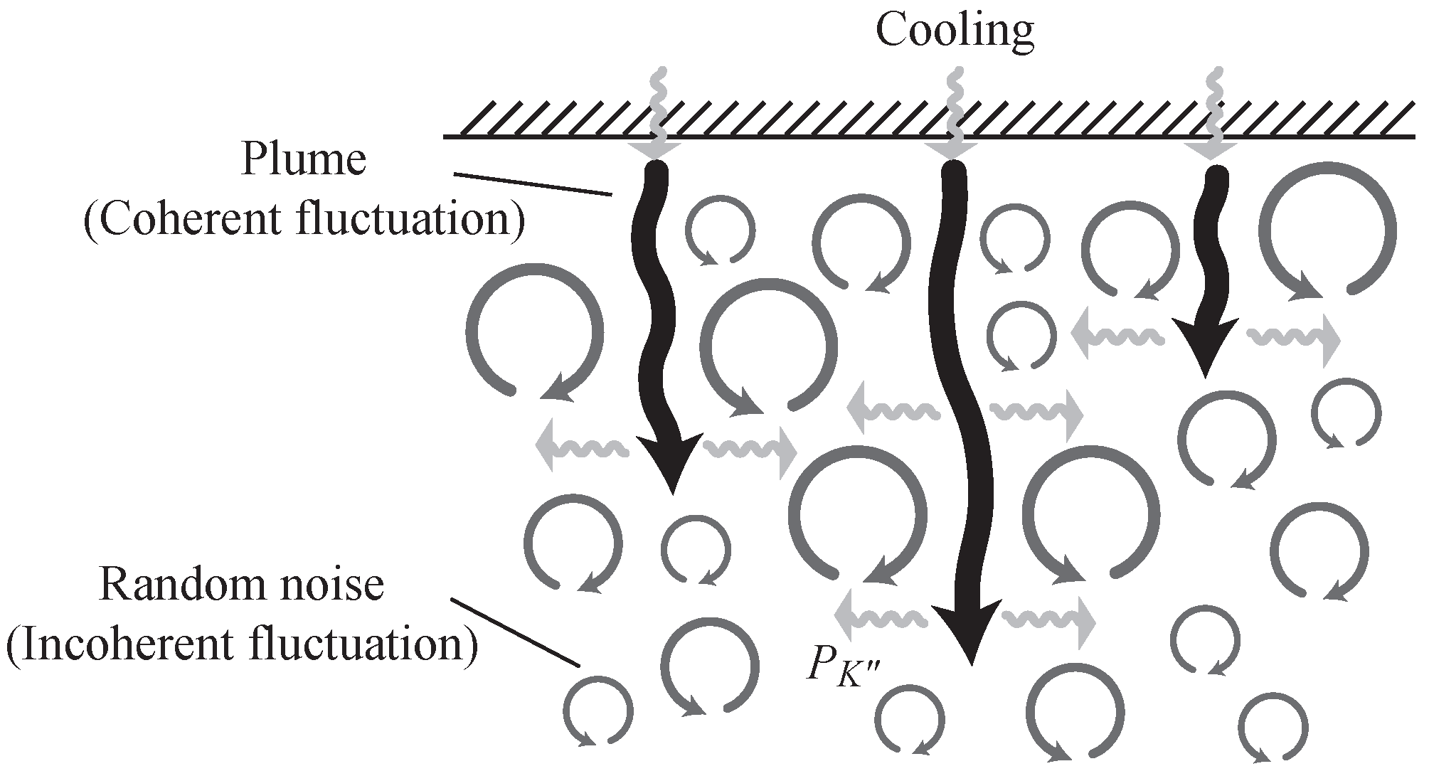
As (66) shows, the sink of the coherent fluctuation energy, $P_{\tilde{K}}<0$, corresponds to the production of the incoherent fluctuation energy, $P_{K^{″}}>0$. In this case, the kinetic energy of the plume or coherent fluctuation motion driven by the surface cooling is transferred towards the kinetic energy of the random or incoherent fluctuation motions as schematically depicted in Figure 6.

In this picture, the diving plumes driven by the surface cooling enhances the turbulent transport through the non-equilibrium effect along the plume motions. During this process, the energy of plumes (coherent fluctuations) is transferred to the energy of random noises (incoherent fluctuations) through the inhomogeneous motions of plumes $\mathsf{\nabla }\tilde{\mathbf{u}}$ coupled with the incoherent fluctuations $\widetilde{{\mathbf{u}}^{″}{\mathbf{u}}^{″}}$. Of course, there are several other mechanisms such as the production $P^{″}$, dissipation ${\epsilon }^{″}$, etc. in (65), that contribute to the evolution of the incoherent fluctuation energy $\langle {\mathbf{u}}^{″}{}^2\rangle$. In this sense, the present picture is a fairly simplified one.

With the non-equilibrium effect, the energy transfer rate to the incoherent component of the fluctuation is written as

$$P_{K^{″}}=-〈\widetilde{u^{″}{}^{\mathsf{\ell }}{u}^{″}{}^m}\frac{\partial {\tilde{u}}^m}{\partial x^{\mathsf{\ell }}}〉\simeq +\tilde{\nu }\left(1-{\tilde{\mathsf{\Lambda }}}_{\mathrm{D}}\right){\left(\frac{\partial {\tilde{u}}^m}{\partial x^{\mathsf{\ell }}}\right)}^2.$$

(69)

As the DNSs of the surface cooling case show (Figure 4), the non-equilibrium-effect coefficient ${\tilde{\mathsf{\Lambda }}}_{\mathrm{D}}$ is negative:

$${\tilde{\mathsf{\Lambda }}}_{\mathrm{D}}<0.$$

(70)

In this case, the energy transfer to the incoherent or random fluctuation is enhanced by the non-equilibrium turbulence effect along the plume motion. This matches the tendency of the surface cooling-driven convection case. The presence of the diving plumes strongly enhances the turbulence mixing through the non-equilibrium effect. This picture is based on several simplifications, but still suggests the importance of the non-equilibrium effect associated with the plume motions in the turbulent transport in convection.

6. Conclusions

Linear gradient-transport-type turbulence models for the turbulent fluxes with the eddy viscosity and diffusivity representation work poorly in some turbulent flows. For example, the K–$\epsilon$ turbulence model based on the eddy viscosity ${\nu }_{\mathrm{T}}=C_{\nu }{K}^2/\epsilon$ cannot be applied to the homogeneous-shear turbulence; it leads to the overestimation of K and $\epsilon$. Convective turbulence with plumes/jets and supersonic turbulence accompanying shocks constitute other examples. Simulations with a simple linear model provide substantially over- or underestimated turbulent transports (turbulent viscosity, mass flux, heat flux, etc.). To rectify this deficiency of linear gradient-transport models, in this work, the non-equilibrium effect mediated by the streamwise variation in turbulence are incorporated into the turbulence model. A turbulence model with these effects implemented in combination was proposed. In the model, in addition to the usual eddy viscosity and diffusivity representations for the turbulent transports, deviations from the simple representations due to the non-equilibrium effect are taken into account.

Relevance of the non-equilibrium effects was argued with utilizing recent elaborated experiments in turbulent jets and plumes. It was pointed out that the expected results of the non-equilibrium effect on turbulent transports in the turbulent jets and plumes are transport enhancement or suppression due to the non-equilibrium effect (depending on the turbulence variation along the jets/plumes). These evaluations of turbulent transports seem to be in preferable directions to correct the discrepant results obtained from simple conventional gradient-transport-type models.

References

- Launder, B.E.; Spalding, D.B. Lectures in Mathematical Models of Turbulence; Academic Press: London, UK, 1972. [Google Scholar]
- Rodi, W. Turbulence Models and Their Application in Hydraulics: A State-of-the-Art Review, 3rd ed.; Taylor and Francis: London, UK, 2000. [Google Scholar]
- Yokoi, N. Turbulence, transport and reconnection. In Topics in Magnetohydrodynamic Topology, Reconnection and Stability Theory: CISM International Centre for Mechanical Sciences, 591; MacTaggart, D., Hillier, A., Eds.; Springer: Berlin/Heidelberg, Germany, 2020; pp. 177–265. [Google Scholar]
- Yokoi, N.; Yoshizawa, A. Statistical analysis of the effects of helicity in inhomogeneous turbulence. Phys. Fluids A 1993, 5, 464–477. [Google Scholar] [CrossRef]
- Yokoi, N.; Brandenburg, A. Large-scale flow generation by inhomogeneous helicity. Phys. Rev. E 2016, 93, 033125. [Google Scholar] [CrossRef] [PubMed] [Green Version]
- Yoshizawa, A.; Nisizima, S. A non-equilibrium representation of the turbulent viscosity based on the two-scale turbulence theory. Phys. Fluids A 1993, 5, 3302–3304. [Google Scholar] [CrossRef]
- Kraichnan, R.H. The structure of isotropic turbulence at very high Reynolds numbers. J. Fluid Mech. 1959, 5, 497–543. [Google Scholar] [CrossRef] [Green Version]
- Edwards, S.F. The statistical dynamics of homogeneous turbulence. J. Fluid Mech. 1964, 18, 239–273. [Google Scholar] [CrossRef]
- Herring, J.R. Self-consistent-field approach to turbulence theory. Phys. Fluids 1965, 8, 2219–2225. [Google Scholar] [CrossRef]
- Herring, J.R. Self-consistent-field approach to nonstationary turbulence. Phys. Fluids 1966, 9, 2106–2110. [Google Scholar] [CrossRef]
- Spruit, H.C. Convection in stellar envelopes: A changing paradigm. Mem. Soc. Astron. Ital. 1997, 68, 397–413. [Google Scholar]
- Rast, M.P. Compressible plume dynamics and stability. J. Fluid Mech. 1998, 369, 125–149. [Google Scholar] [CrossRef]
- Cossette, J.-F.; Rast, M.P. Supergranulation as the largest buoyant driven convective scale of the Sun. Astrophys. J. Lett. 2016, 829, L17. [Google Scholar] [CrossRef] [Green Version]
- Brandenburg, A. Stellar mixing length theory. Astrophys. J. 2016, 832, 6. [Google Scholar] [CrossRef] [Green Version]
- Bethe, H.A.; Wilson, J.R. Revival of stalled supernova shock by neutrino heating. Astrophys. J. 1985, 295, 14–23. [Google Scholar] [CrossRef]
- Couch, S.M.; Warren, M.L.; O’Connor, E.P. Simulating turbulence-aided neutrino-driven core-collapse supernova explosions in one dimension. Astrophys. J. 2020, 890, 127. [Google Scholar] [CrossRef]
- Janka, H.-T.; Müller, E. Neutrino heating, convection, and mechanism of Type-II supernova explosions. Astron. Astrophys. 1996, 306, 167–198. [Google Scholar]
- Mabanta, J.W.; Murphy, Q.A. How turbulence enables core-collapse supernova explosion. Astrophys. J. 2018, 856, 22. [Google Scholar] [CrossRef] [Green Version]
- Marek, A.; Janka, H.-T. Delayed neutrino-driven supernova explosions aided by the standing accretion-shock instability. Astrophys. J. 2009, 694, 664–696. [Google Scholar] [CrossRef] [Green Version]
- Müller, B. A critical assessment of turbulence models for 1D core-collapse supernova simulations. Mon. Not. R. Astron. Soc. 2019, 487, 5304–5323. [Google Scholar] [CrossRef] [Green Version]
- Murphy, Q.A.; Meakin, C. A global turbulence model for neutrino-driven convection in core-collapse supernovae. Astrophys. J. 2011, 742, 74. [Google Scholar] [CrossRef]
- Layek, G.C.; Sunita, V. Non-Kolmogorov scaling and dissipation laws in planar turbulent plume. Phys. Fluids 2018, 30, 115105. [Google Scholar] [CrossRef]
- Cafiero, G.; Vassilicos, J.C. Nonequilibrium turbulence scalings and self-similarity in turbulent planar jets. Proc. R. Soc. Lond. A 2019, 475, 20190038. [Google Scholar]
- Sunita, V.; Layek, G.C. Nonequilibrium turbulent dissipation in buoyant axisymmetric plume. Phys. Rev. Fluids 2021, 6, 104602. [Google Scholar] [CrossRef]
- Bordoloi, A.D.; Lai, C.C.K.; Clark, L.; Veliz, G.; Variano, E. Turbulence statistics in a negatively buoyant multiphase plume. J. Fluid Mech. 2020, 896, A19. [Google Scholar] [CrossRef]
- Charonko, J.J.; Prestridge, K. Variable-density mixing in turbulent jets with coflow. J. Fluid Mech. 2017, 825, 887–921. [Google Scholar] [CrossRef]
- Lai, C.C.K.; Socolofsky, S.A. Budgets of turbulent kinetic energy, Reynolds stresses, and dissipation in a turbulent round jet discharged into a stagnant ambient. Environ. Fluid Mech. 2019, 19, 349–377. [Google Scholar] [CrossRef]
- Lai, C.C.K.; Socolofsky, S.A. The turbulent kinetic energy budget in a bubble plume. J. Fluid Mech. 2019, 865, 993–1041. [Google Scholar] [CrossRef]
- Yokoi, N.; Masada, Y.; Takiwaki, T. Modelling stellar convective transport with plumes—I. Non-equilibrium turbulence effect in double-averaging formulation. Mon. Not. R. Astron. Soc. 2022, 516, 2718–2735. [Google Scholar] [CrossRef]
- Yoshizawa, A. Statistical analysis of the deviation of the Reynolds stress from its eddy-viscosity representation. Phys. Fluids 1984, 27, 1377–1387. [Google Scholar] [CrossRef]
- Yoshizawa, A. Hydrodynamic and Magnetohydrodynamic Turbulent Flows: Modeling and Statistical Theory; Kluwer: Dordrecht, The Netherlands, 1998; pp. 265–303. [Google Scholar]
- Yokoi, N. Cross helicity and related dynamo. Geophys. Astrophys. Fluid Dyn. 2013, 107, 114–184. [Google Scholar] [CrossRef] [Green Version]
- Yokoi, N. Electromotive force in strongly compressible magnetohydrodynamic turbulence. J. Plasma Phys. 2018, 84, 735840501. [Google Scholar] [CrossRef]
- Yokoi, N. Mass and internal-energy transports in strongly compressible magnetohydrodynamic turbulence. J. Plasma Phys. 2018, 84, 735840603. [Google Scholar] [CrossRef]
- Okamoto, M. Theoretical investigation of an eddy-viscosity-type representation of the Reynolds stress. J. Phys. Soc. Jpn. 1994, 63, 2101–2122. [Google Scholar] [CrossRef]
- Tennekes, H.; Lumley, J.L. A First Course in Turbulence; The MIT Press: Cambridge, MA, USA, 1972. [Google Scholar]
- Livescu, D.; Ristorcelli, J.R. Variable-density mixing in buoyancy-driven turbulence. J. Fluid Mech. 2008, 605, 145–180. [Google Scholar] [CrossRef]
Figure 1.
Schematically depicted evolution of the turbulent energy in the simulations of homogeneous-shear flow. •: DNS, : standard K– model simulation; and ―: non-equilibrium model simulation. Onset of the model simulations is set at a scaled time using the DNS data (S: shear rate).
Figure 2.
The non-equilibrium effect associated with a plume motion. A plume is thermobuoyantly formed above a heat source. The non-equilibrium effect is taken into account through the Lagrangian or advective derivatives of the turbulent energy K and its dissipation rate , and , where is the plume velocity.
Figure 3.
Entropy distributions in the direct numerical simulations (DNSs) for the locally driven case (a) and the non-locally driven case (b). The horizontal cross-sections of the entropy fluctuation at the top surface (Top). In the non-locally or cooling-driven case, the horizontal extension of the cell structures is much more limited than the counterpart in the locally driven case. The vertical cross-sections of the entropy fluctuation from the horizontal mean (bottom). In the non-locally driven case, the low-entropy down flow or plume structures produced at the surface are prominent in the upper region.
Figure 4.
Spatial distributions of the non-equilibrium effect factor . The left axis is the depth from the surface (). The magnitude of the non-equilibrium effect factor depends on the time averaging window T.
Figure 5.
Spatial distributions of the turbulent internal-energy flux obtained by the direct numerical simulations (DNSs) and the model with the non-equilibrium effect. The left axis is the depth from the surface (). The DNS results for the locally driven convection case (⋯), for the non-locally driven convection case () and the result from the model with the non-equilibrium effect for the non-locally driven convection case (―).
Figure 6.
Schematic picture of the interaction between the coherent and incoherent fluctuations. Plumes (coherent fluctuations, depicted by thick black curved lines) are driven by the surface cooling. The energy of the plume motions are transferred to the energy of the random noise (incoherent fluctuation, depicted by gray circle eddies) by the interaction if .