Article

A Parametric Model of Elliptic Orbits for Annual Evolutions of Northern Hemisphere Stratospheric Polar Vortex and Their Interannual Variability

1
Key Laboratory of Meteorological Disaster, Ministry of Education (KLME)/Joint International Research Laboratory of Climate and Environment Change (ILCEC)/Collaborative Innovation Center on Forecast and Evaluation of Meteorological Disasters (CIC-FEMD), Nanjing University of Information Science & Technology, Nanjing 211544, China
2
State Key Laboratory of Numerical Modeling for Atmospheric Sciences and Geophysical Fluid Dynamics (LASG), Institute of Atmospheric Physics, Chinese Academy of Sciences, Beijing 100029, China
3
Department of Earth, Ocean & Atmospheric Sciences, Florida State University, Tallahassee, FL 32304, USA
4
Reading Academy, Nanjing University of Information Science & Technology, Nanjing 210044, China
*
Author to whom correspondence should be addressed.
Atmosphere 2023, 14(5), 870; https://doi.org/10.3390/atmos14050870
Submission received: 12 April 2023 / Revised: 11 May 2023 / Accepted: 12 May 2023 / Published: 14 May 2023

Abstract

:
The year-to-year varying annual evolutions of the stratospheric polar vortex (SPV) have an important downward impact on the weather and climate from winter to summer and thus potential implications for seasonal forecasts. This study constructs a parametric elliptic orbit model for capturing the annual evolutions of mass-weighted zonal momentum at 60° N (MU) and total air mass above the isentropic surface of 400 K (M) over the latitude band of 60–90° N from 1 July 1979 to 30 June 2021. The elliptic orbit model naturally connects two time series of a nonlinear oscillator. As a result, the observed coupling relationship between MU and M associated with SPV as well as its interannual variations can be well reconstructed by a limited number of parameters of the elliptic orbit model. The findings of this study may pave a new way for short-time climate forecasts of the annual evolutions of SPV, including its temporal evolutions over winter seasons as well as the spring and fall seasons, and timings of the sudden stratospheric warming events by constructing its elliptic orbit in advance.

1. Introduction

The Northern Hemisphere stratospheric polar vortex (SPV) is characterized by a significant annual evolution or annual cycle [1]. It spins up from autumn and persists through winter into spring, at which point it breaks up and the typical wintertime subpolar westerlies are replaced by easterly summer circulation until the subsequent autumn [2,3]. The transition from a winter to a summer circulation regime is known as the stratospheric final warming (SFW) [4], which is influenced by both solar radiation and dynamics [5].
There are various indices commonly used to describe the strength of the stratospheric polar vortex. These indices include polar cap (60–90° N) height [6], polar cap temperature, potential vorticity on isentropic surfaces [7,8,9], polar mass [10], zonal-mean zonal wind at subpolar latitudes [11,12,13] and Northern Annular Mode (NAM) [14,15,16,17]. Baldwin and Thompson [18] have made a comprehensive comparison among those indices and found that these indices generally correspond well with each other and are capable of representing the variability in the SPV. The anomalous changes in these indicators always exhibit remarkably larger amplitudes from late fall to early spring each year and are dominated by intra-seasonal variabilities [14,15,19,20].
The dynamic influence of the stratospheric polar vortex during the winter months is known to play a part in shaping the winter circulation patterns of the troposphere such as Arctic Oscillation and blockings [17,20,21,22,23,24,25,26]. As a result, the anomalous signals in the stratospheric polar vortex can exert important downward impacts on weather and climate in the extratropical troposphere. For instance, during the 1–2 months after a weaker stratospheric polar vortex event such as sudden stratospheric warming (SSW) and negative stratospheric northern annular mode event, below-normal temperatures tend to occur more frequently over the Northern Hemispheric continents [24,27,28,29,30,31,32,33,34,35,36,37,38]. In addition, the polar temperature related to the SPV in the late winter months is closely related to the formation of polar stratospheric clouds and thus affects the Arctic ozone depletion [39,40,41,42]. The interannual variations in seasonal timing and the features of stratospheric final warming have been found to affect the spring circulation anomalies, which in turn modifies the summer monsoon [4,43], and affect precipitation anomalies over South Asia in May and the temperature anomalies over Central Asia in March [44]. Later, stratospheric final warming and stronger SPV in springtime have also been found to lead to negative ice thickness anomalies in the East Siberian Sea [3]. The strength of SPV can be the sub-seasonal to seasonal forewarning of anomalous atmospheric river frequency [45]. Therefore, identifying and understanding the year-to-year varying annual cycle of SPV has potential implications for winter seasonal forecasts, as the December–February mean behavior may miss important sub-seasonal events.
Hardiman et al. [46] formulate a simple sine wave fit to the observed vacillations in the daily zonal, mean zonal wind anomalies at 10 hPa, which can be used to explain much of the sub-seasonal and interannual variability in the monthly mean vortex strength. Additionally, consistent with wave-mean flow interaction theory, their amplitude correlates positively with the magnitude of winter mean planetary wave driving. They then tested the predictive skill of this simple sine wave model throughout the winter against the persistence of the vortex strength and against a state-of-the-art seasonal forecasting system, and reported improved prediction skills of the vortex strength one month ahead.
Not only the zonal wind surrounding the SPV but also the thermal condition in the stratospheric polar region are important indicators of the SPV intensity changes. The changes in momentum and thermal fields associated with SPV variations are intimately coupled as expected from the thermal wind relationship. According to Zuev and Savelieva [47], the temperature distribution inside the SPV at a specific range of wind speed was approximately in the same temperature range, but the temperature clearly shows year-to-year differences. This study formulates a parametric ellipse orbit model for better capturing the coupled annual evolutions of both the zonal momentum of the polar jet and the total air mass in the polar cap of the stratosphere and their interannual variability.

2. Data and Methods

2.1. Data

Daily mean fields are derived from the hourly ERA5 reanalysis dataset [48], which is on 1.5° × 1.5° grids and covers 42 years (July of the previous year to June of the current year) from 1979/80 to 2020/21. We use variables including the three-dimensional temperature, geopotential height and wind fields at 37 pressure levels from 1000 hPa to 1 hPa, air pressure, 2 m air temperature and wind fields at the surface. A 7-day running mean is applied to minimize synoptic-scale perturbations.

2.2. Methods

In this study, we use the stratospheric polar mass (M) above the isentropic surface of 400 K inside the Arctic polar circle and mass-weighted zonally integrated zonal momentum at 60° N (MU) to represent the polar vortex and polar jet changes. The isentropic level 400 K is about 100 hPa in the subpolar latitudes. This level is chosen in our study because the stratospheric circulation signals above 400 K can actively interact with the upward propagating tropospheric waves [49,50,51,52,53,54,55,56], which in turn exert significant downward impacts on the tropospheric circulation and the weather in winter [19,57,58]. The latitude of 60° N is chosen to better capture the edge of the stratospheric polar vortex and the maximum of the westerly surrounding the vortex in the winter seasons. These two variables are addable and closely linked to the mass budget and angular momentum budget [10,26,59], and thus can be quantitatively attributed to the adiabatic processes mainly driven by wave dynamics and diabatic processes.
Following Pauluis et al. [60,61] and Yu et al. [10,62], we first interpolated the daily potential temperature and wind fields onto 200 equally spaced sigma (σ) levels from 1 to 0. The air mass between two adjacent sigma surfaces per unit area is m σ   = Δσ/g Ps, where g is the gravitational constant, Δσ = 1/200 and Ps is the surface pressure. According to Yu et al. [10], the M can be measured by the integrated mass above 400 K isentropic level north of 60° N (kg), which is derived as
M ( t ) = π / 3 π / 2 0 2 π 0 1 m σ ( λ ,   ϕ , σ , t ) · H ( θ ( λ ,   ϕ , σ , t ) , 400   K ) d σ Rcos ϕ d λ Rd ϕ
where λ is the longitude and ϕ is the latitude, R is the Earth radius; H is the Heaviside function, namely H(x, x0) = 1 if x   x 0, and otherwise H(x,x0) = 0. In (1) and (2) below, x = θ(λ,φ,σ,t) and x0 = 400 K.
Similarly, the intensity of the polar jet can be measured by the zonally integrated zonal momentum in the stratospheric layer above 400 K across 60° N (MU, unit: kg m s−1), which can be obtained according to
M U ( t ) = 0 2 π 0 1 m σ ( λ ,   ϕ = 60   N , σ , t ) · u ( λ ,   ϕ = 60   N , σ , t ) · H ( θ ( λ ,   ϕ = 60   N , σ , t ) , 400   K ) d σ Rcos ϕ d λ
Smaller values of M indicate a stronger stratospheric polar vortex, while larger values of MU indicate a stronger polar jet and vice versa.

3. Results

3.1. Statistics of the SPV Indices

From the annual evolutions (Figure 1), we see that the stratospheric mass in the polar region (M) and the relative zonal momentum around the polar jet (MU) vary generally out of phase. Namely, the MU increases while the M decreases before February and then the MU decreases while the M increases afterward. This illustrates that the Northern Hemisphere SPV and the polar jet surrounding it persist in the winter months and peak around mid-January. Radiative heating/cooling processes provide overall control of the annual cycle of M thermodynamically and adiabatic eddy-driven poleward mass transport processes affect the amplitude and phase of the annual cycle dynamically. The annual cycle of MU, besides through the thermal wind balance which is a fast process (less than a day), is controlled by planetary-scale waves that drive the poleward mass transport in the first place. Specifically, a stronger (weaker) poleward transport tends to coincide with the weakening (strengthening) of MU, which is about a few days prior to the increase in M [10]. In other words, at seasonal scales, the annual cycle of MU is driven by the radiative processes via thermal wind balance. However, at sub-seasonal time scales, particularly in the winter seasons, temporal evolutions of MU are driven by planetary-scale waves, which in turn drive the temporal evolution of M through eddy-driven poleward mass transport. The standard deviations of MU and M become remarkably larger in the months from December to March compared to the other months throughout the year, consistent with previous studies [14,15,19,20]. Note that the MU shows larger interannual variations around its climatology than the M. In particular, the maximum standard deviation of MU during the winter months is around 60% of its climatological mean, while for the M, its maximum standard deviation is only about 10% of its climatological mean. The seasonal changes of the coupled M and MU also exhibit remarkable interannual variation, as can be seen clearly from Figure 2. The timing of the strongest SPV, which can be represented by the minimum M and maximum MU, ranges from December to April, during the period from 1980 to 2020.
A closer look at the temporal evolutions of the M and MU in a few selected years (Figure 3) reveals that MU leads M by a few days, even though they are generally negatively correlated. We then investigate the lead–lag correlations of M and MU in each year and the lead days of the MU relative to the M when their maximum negative correlations are reached (Figure 4). It is seen that the maximum negative correlations occur mostly when the MU leads the M. The lead time is mainly in the range of 1–10 days with a climatological mean value of about a week. As discussed above, it is the planetary-scale wave activity that drives the temporal evolutions of MU, which in turn leads to changes in the M field with a lead-time of a few days [10]. Therefore, temporal evolutions of M at sub-seasonal time scales are strongly modulated by eddy-driven poleward energy transport.
In summary, the observed annual evolutions of M and MU, respectively, representing the changes in the thermal and dynamical conditions of the SPV throughout the year, have three main features: (i) the M and MU are dominated by the annual cycle with the largest interannual variability in winter; (ii) the MU has a larger interannual variability than the M; and (iii) the MU varies out of phase with the M but with MU leads to M by 1–10 days.

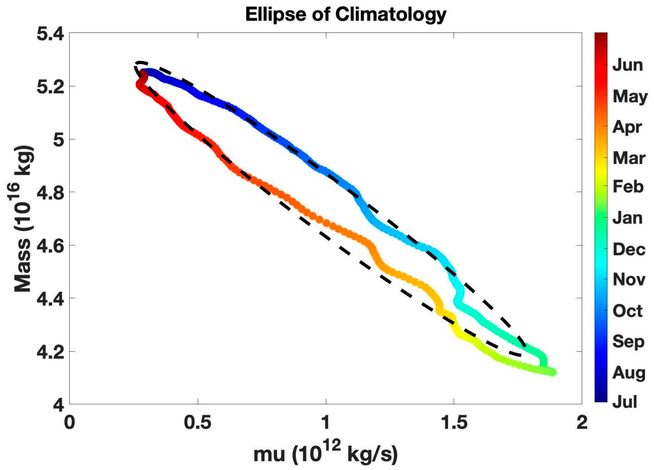
3.2. The Parametric Elliptic Orbit Model

In this section, we will construct a parametric model of elliptic orbits to capture the coupled changes of the M and MU. To begin with, because the annual cycle of the M or the MU is close to a sine or cosine function, we can first formulate two variables, X, and Y, as
{ X = X 0 + a cos Θ cos α + b sin Θ sin α Y = Y 0 + a cos Θ sin α b sin Θ cos α
where X0 and Y0 are the coordinates of the elliptic central point; a and b are the amplitudes; Θ is the phase angle in the range from 0 to 2 π ; and a corresponds to the tilting angle of the elliptic obit with the x-axis ranging from − π to π . The other form of (3) is the familiar elliptic equation, namely
( X X 0 ) 2 a 2 + ( Y Y 0 ) 2 b 2 = 1
Displayed in Figure 5 is an idealized elliptic orbit with α = 0.25 π . It is seen that when the Θ increases from 0 to π , X increases to a maximum while Y decreases to a minimum. Then, from Θ   = π to 2 π , X decreases to minimum while Y increases to maximum. If we consider MU as the X and M as the Y, such changes that accompany Θ = 0 to 2 π are quite consistent with their annual cycle from the previous year, from summer to winter and then to the concurrent summer.
According to the parametric elliptic orbit model, the maximum negative correlations between X and Y can occur at different lead-lag times, which highly depend on the ratio b/a and the angle α . For the α in the range of 0~ π 2 , a larger b/a would yield a longer lead time for the X relative to Y to achieve their maximum negative correlation. Contrarily, for the α in the range of π 2 ~ π , a smaller b/a would yield a longer lead time for the X relative to Y.
We apply a MATLAB function, “fit_ellipse” to a pair of daily time series of MU and M from 1 July to 30 June of the next year to determine the parameters X0, Y0, a, b and α with Θ = 2 π t 365   , where t starts on 1 July as t = 1 and ends on June 30 as t = 365 (29 February in a leap year is excluded in our analysis). The information from “fit_ellipse” can be found at https://www.mathworks.com/matlabcentral/fileexchange/3215-fit_ellipse (accessed on 15 January 2023). To better capture the observed lead time information of MU with respect to M, we introduce an auxiliary equation when applying the “fit_ellipse” function such that the constructed time series of MU and M from the fitted elliptic orbit meet the same lead time of the observed MU with respect to the observed M. As illustrated in Figure 5, when the value of α is fixed, the lead-lag days of maximum correlation and the ratio b/a have a one-to-one correspondence relation. The climatological mean annual cycles of MU and M and their elliptic orbit are displayed in Figure 6. The close resemblance between the fitted orbit elliptic (dashed magenta) and the scattering plot of the observed MU and M (colored dots) indicates that an elliptic orbit is capable of capturing the annual evolutions of MU and M. In particular, the fitted MU also varies out of phase with the fitted M.

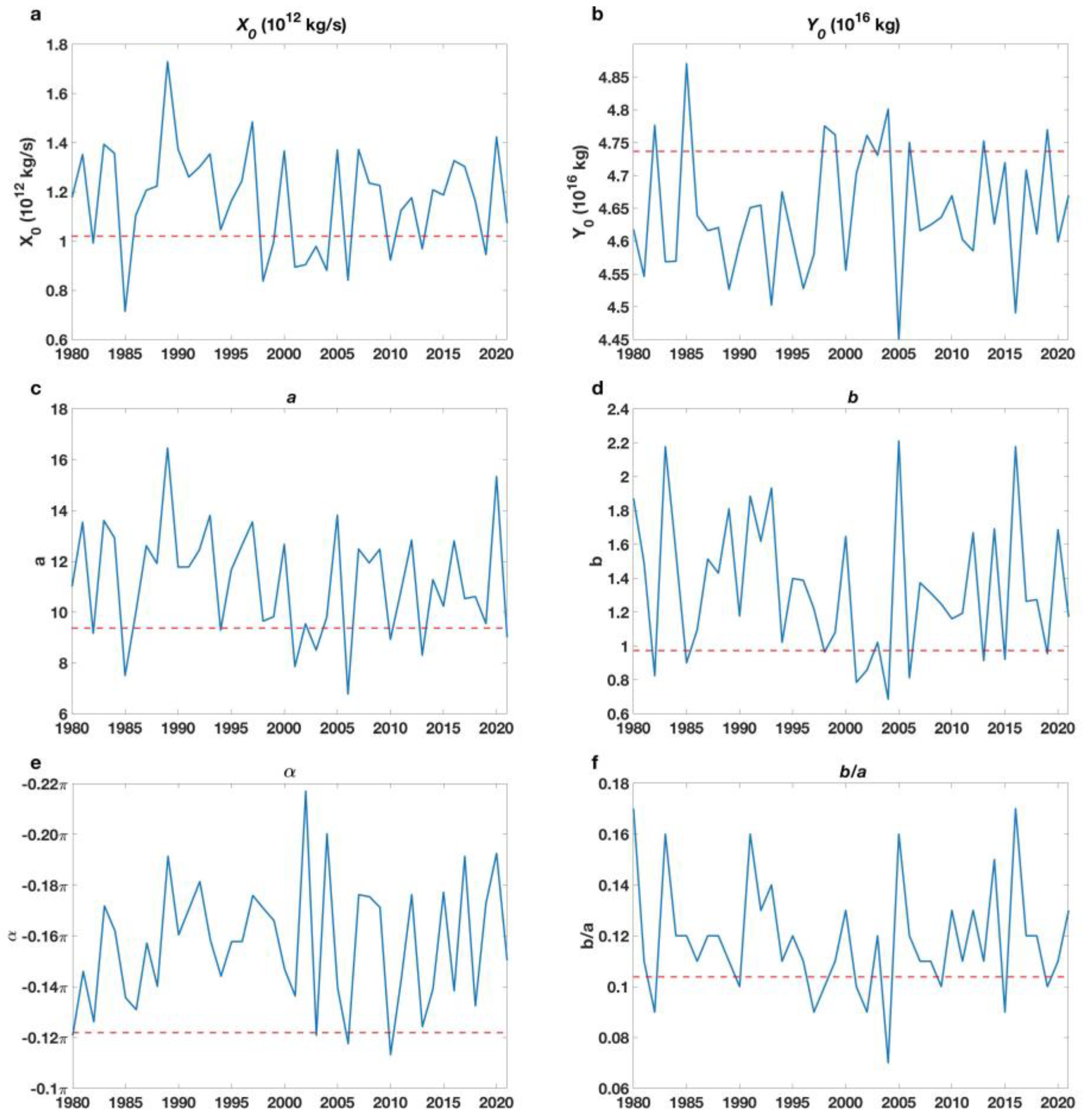
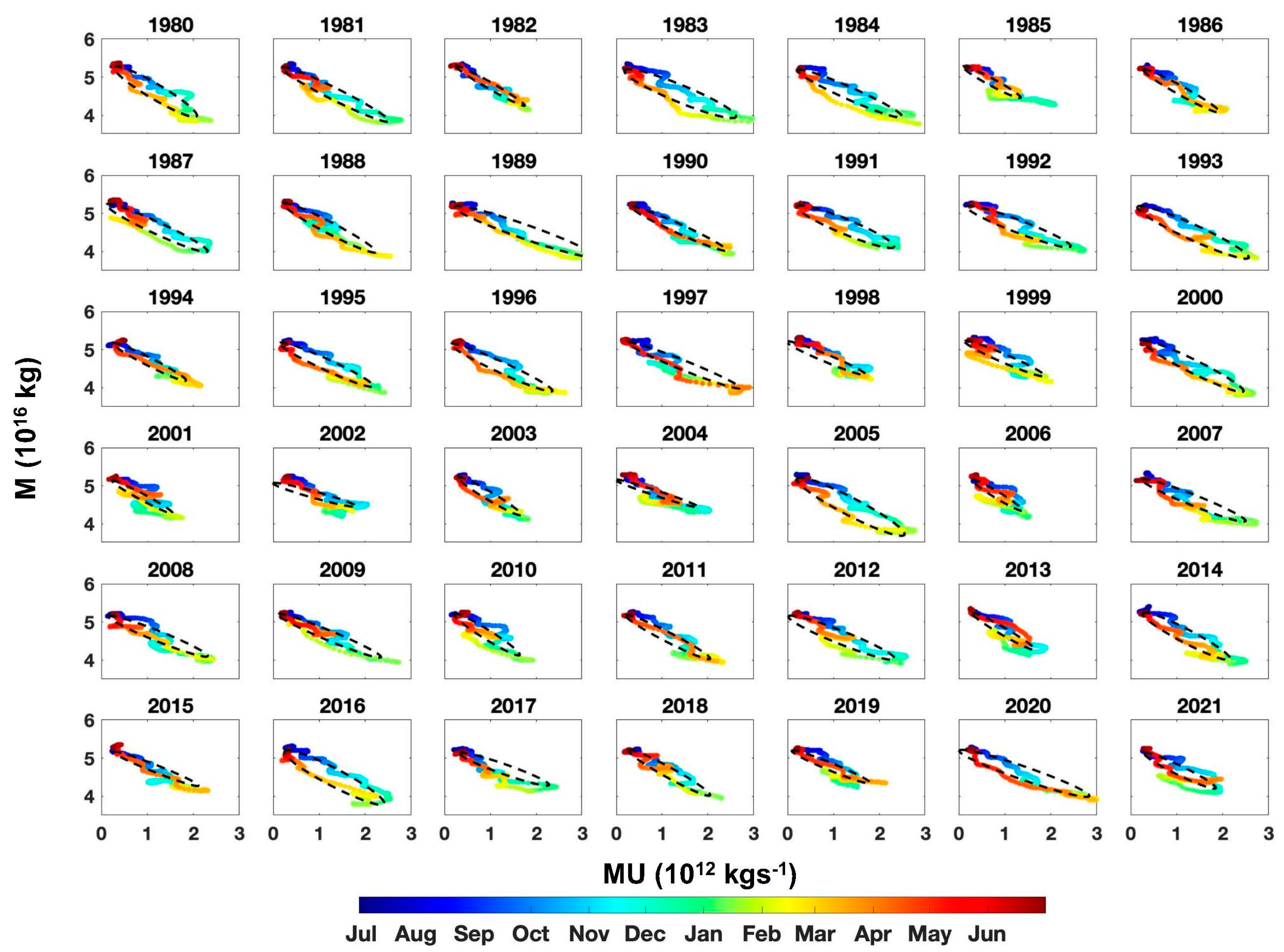
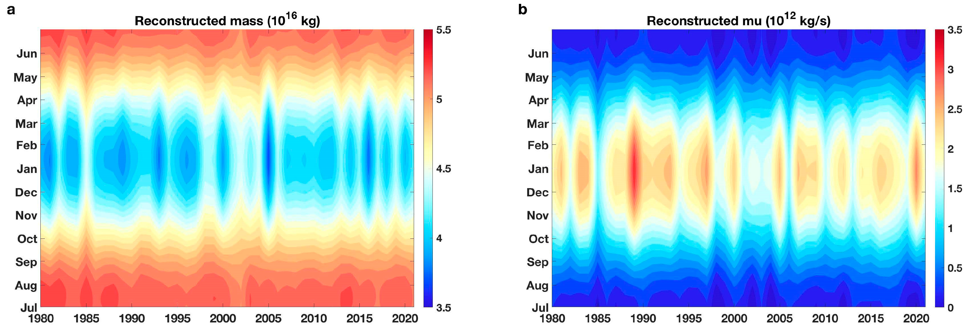
3.3. Year-to-Year Variations of the Elliptic Orbits for the Annual Evolutions of M and MU

In this section, we will examine the effectiveness of the parametric elliptic orbit model in capturing the inter-annual variations in the annual evolutions of the MU and M. The yearly time series of the parameters derived from the ellipse orbit fitting function are shown in Figure 7. It is seen that each of these yearly time series exhibits a strong year-to-year variability. In particular, they have pronounced differences to their counterparts derived from the climatological orbit (dashed magenta), indicating a strong year-to-year variation in the elliptic orbits. The generally larger values of X0 and smaller values of Y0 than their counterparts for the climatological elliptic orbit are observed, and the general out-of-phase relationship between MU and M is also present in the year-to-year variation in their annual means. The generally larger values of a and b than their climatological counterparts indicate that the amplitudes of the seasonal cycles of individual years are stronger than those of the climatological annual cycle. The generally larger values of b/a and α than their climatological counterparts indicate that the lead days of MU with respect to M in individual years are longer than for their climatological counterpart.
It is seen from Figure 8 that the fitted elliptic orbits of individual years exhibit similar patterns to the yearly scatter plots of MU versus M in terms of both timing and intensity. In particular, the fitted orbits capture faithfully the interannual variations in extreme values of both MU and M in the winter seasons. For example, the fitted orbits capture the weaker SPV in the winters of 1982/83, 2001/02, 2002/03, 2003/04, 2006/07 and 2013/2014, which correspond to the panels in Figure 8 (or the abscissa’s tick marks in Figure 9), labeled as 1982, 2001, 2003, 2006 and 2013, respectively. The year-to-year annual evolutions of MU and M obtained from the fitted elliptic orbits are shown in Figure 9. In comparison with Figure 2, it can be seen that the fitted elliptic orbits can capture both the annual evolutions and their interannual variability in MU and M, as well as the generally negative correlation between MU and M at both intraseasonal and interannual scales.
Next, we quantitatively compare the extremes of MU and M in the winter seasons and their annual-cycle amplitudes obtained from the fitted orbits with the original time series of MU and M. Figure 10a,b shows that the yearly extreme values of both MU and M in winter seasons obtained from the fitted orbits have a high positive correlation (exceeding 0.94) with their counterparts obtained from the 31-day running mean time series of observed MU and M. The slightly larger values of the maximum MU and minimum M indicate that the fitted orbits tend to overestimate the strength of SPV in the winter seasons. The year-to-year variations in the amplitude of the annual cycle of MU and M (defined as the differences between the maximum and minimum values in the annual evolutions of MU and M) are displayed in Figure 10c,d, where the orbit-fitted amplitudes are compared with the observed ones. The figures show that the fitted orbits can almost perfectly capture the observed year-to-year variations in the annual cycle amplitudes for both MU and M, as is evident from the positive correlation exceeding 0.9. Next, we examine if the parametric elliptic orbit model can faithfully reflect the coupling between MU and M at the interannual time scale, as it does at the annual time scales (e.g., Figure 9 versus Figure 2). Figure 10e shows the scatter plot of the yearly time series of maximum MU and minimum M, which jointly measure the year-to-year variations in the strength of the SPV in the winter seasons. It is seen that the correlation between the yearly time series of MU and M derived from the fitted orbits (red circles) is identical to that derived from the observations (blue circles), equaling −0.78. Therefore, the observed negative correlation between the interannual variability in MU and that in M is well captured by the fitted orbits. Figure 10f shows the scatter plot of the yearly time series of the amplitude of the annual evolutions of MU and M. The observations show that the annual evolution amplitude of MU of individual years is positively and strongly correlated with that of M (about 0.69) and so are the fitted orbits (0.72) and the observation (0.69). It can be summarized from Figure 8, Figure 9 and Figure 10 that both the annual evolutions and their yearly variations in MU and M are well coupled with significant correlations (about or larger than 0.7), which can be captured with almost identical correlations by the orbit fitting method, with five parameters varying yearly, as illustrated in Figure 7.

4. Conclusions

The year-to-year varying annual evolutions of the stratospheric polar vortex (SPV) have an important downward impact on the weather and climate from winter to summer and thus potential implications for seasonal forecasts. This study considers the necessity of investigating both the thermal and dynamical conditions of SPV by jointly considering the daily time series of the zonally integrated mass-weighted zonal momentum at 60° N (MU) and the total air mass above the isentropic surface of 400 K (M) over the latitude band of 60–90° N. The annual evolutions of MU are characterized by a generally out-of-phase relationship with the annual evolutions of M, and the changes in MU tend to lead the changes in M by 1–10 days. Moreover, their annual evolutions have significant interannual variations, which also exhibit a strong negative correlation between MU and M.
By constructing a parametric elliptic orbit model to fit the daily time series of MU and M in each year, we can closely reproduce the year-to-year variations in the annual evolutions of the observed MU and M jointly from the year-to-year variations in their elliptic orbits, including their amplitude, extremes in winter seasons, as well the strong negative correlation between MU and M and their amplitudes in the annual cycle at the interannual time scales. The findings of this study may pave a new way for short-time climate forecasts of the annual evolutions of SPV, including its temporal evolutions over individual cold seasons (including the spring and fall seasons). In particular, one would be able to predict timings of the minimum MU and maximum M in a given year by predicting the five parameters (X0, Y0, a, b, and α) of the corresponding yearly elliptic orbit. Because the timings of minimum MU and maximum M correspond closely to the timings of SSW events, one could in turn predict the timings of the high probability occurrence of SSW events in winters. Such a circulation condition during this timing would provide a favorable background for the break-up of the stratospheric polar vortex, which may yield a higher probability of the occurrence of SSW, which will be a topic of our future studies.
We here wish to add that this study is focused on the seasonal cycle of the stratospheric polar vortex in the Northern Hemisphere. In the Southern Hemisphere, the annual cycle of the stratospheric polar vortex also plays an important role in extreme surface weather conditions and natural hazards, as it may raise the risk of increased rainfall in the latitudinal band of 35–50° S [63,64,65]. According to previous studies, the Southern Hemisphere stratospheric polar vortex tends to be steadier and varies at a longer period [9,66] and break-up events occur less frequently [65]. It is expected that the annual cycle of the stratospheric polar vortex as well as extreme events such as SSW in the Southern Hemisphere could be also well captured by our parametric elliptic orbit model, which will be verified in our future work.

Author Contributions

Conceptualization, M.C. and Y.Y.; methodology, Y.Y.; validation, J.S., M.S. and Y.Y.; formal analysis, J.S. and M.S.; investigation, M.C.; data curation, J.S.; writing—original draft preparation, Y.Y.; writing—review and editing, M.C., J.S., M.S. and X.L.; visualization, J.S.; supervision, M.C.; project administration, M.C.; funding acquisition, M.C. and Y.Y. All authors have read and agreed to the published version of the manuscript.

Funding

This research was jointly funded in part by the National Science Foundation of China, grant number 42075052, and the Natural Science Foundation of Jiangsu Province, grant number BK20211288, Climate Program Office of National Oceanic and Atmospheric Administration (NA20OAR4310380), and the National Science Foundation (AGS-2032542).

Data Availability Statement

Acknowledgments

We would like to thank the three anonymous reviewers for their constructive comments.

Conflicts of Interest

The authors declare no conflict of interest.

References

  1. Hu, J.G.; Ren, R.C.; Yu, Y.Y.; Xu, H.M. The boreal spring stratospheric final warming and its interannual and interdecadal variability. Sci. China Earth Sci. 2014, 57, 710–718. [Google Scholar] [CrossRef]
  2. Schoeberl, M.R.; Newman, P.A. Chapter middle atmosphere: Polar vortex. In Encyclopedia of Atmospheric Sciences, 2nd ed.; North, J.G.R., Pyle, F.Z., Eds.; Academic Press: Cambridge, MA, USA, 2015; Volume 4, pp. 12–17. [Google Scholar]
  3. Kelleher, M.E.; Blanca, A.; James, A.S. Interseasonal Connections between the Timing of the Stratospheric Final Warming and Arctic Sea Ice. J. Clim. 2020, 33, 3079–3092. [Google Scholar] [CrossRef]
  4. Hu, J.G.; Ren, R.C.; Xu, H.M. Occurrence of winter stratospheric sudden warming events and the seasonal timing of spring stratospheric final warming. J. Atmos. Sci. 2014, 71, 2319–2334. [Google Scholar] [CrossRef]
  5. Wei, K.; Wen, C.M.; Huang, R.H. Dynamical diagnosis of the breakup of the stratospheric polar vortex in the Northern Hemisphere. Sci. China-Earth Sci. 2007, 50, 1369–1379. [Google Scholar] [CrossRef]
  6. Cohen, J.; Salstein, D.; Saito, K. A dynamical framework to understand and predict the major Northern Hemisphere mode. Geophys. Res. Lett. 2002, 29, 51. [Google Scholar] [CrossRef]
  7. Cai, M.; Ren, R.C. Meridional and Downward Propagation of Atmospheric Circulation Anomalies. Part I: Northern Hemisphere Cold Season Variability. J. Atmos. Sci. 2007, 64, 1880–1901. [Google Scholar] [CrossRef]
  8. Ren, R.C.; Cai, M. Meridional and vertical out-of-phase relationships of temperature anomalies associated with the Northern Annular Mode variability. Geophys. Res. Lett. 2007, 34. [Google Scholar] [CrossRef]
  9. Ren, R.C.; Cai, M. Meridional and downward propagation of atmospheric circulation anomalies. Part II: Southern Hemisphere cold season variability. J. Atmos. Sci. 2008, 65, 2343–2359. [Google Scholar] [CrossRef]
  10. Yu, Y.; Cai, M.; Ren, R.A. Stochastic model with a low-frequency amplification feedback for the stratospheric northern annular mode. Clim. Dyn. 2018, 50, 3757–3773. [Google Scholar] [CrossRef]
  11. Lorenz, D.J.; Hartmann, D.L. Eddy–zonal flow feedback in the Northern Hemisphere winter. J. Clim. 2003, 16, 1212–1227. [Google Scholar] [CrossRef]
  12. Christiansen, B. Downward propagation and statistical forecast of the near-surface weather. J. Geophys. Res. 2005, 110, D14104. [Google Scholar] [CrossRef]
  13. Christiansen, B. Is the atmosphere interesting? A projection pursuit study of the circulation in the Northern Hemisphere winter. J. Clim. 2009, 22, 1239–1254. [Google Scholar] [CrossRef]
  14. Thompson, D.W.J.; Wallace, J.M. The Arctic Oscillation signature in the wintertime geopotential height and temperature fields. Geophys. Res. Lett. 1998, 25, 1297–1300. [Google Scholar] [CrossRef]
  15. Thompson, D.W.J.; Wallace, J.M. Annular modes in the extratropical circulation. Part I: Month-to-month variability. J. Clim. 2000, 13, 1000–1016. [Google Scholar] [CrossRef]
  16. Limpasuvan, V.; Hartmann, D.L. Wave-maintained annular modes of climate variability. J. Clim. 2000, 13, 4414–4429. [Google Scholar] [CrossRef]
  17. Baldwin, M.P.; Dunkerton, T.J. Stratospheric Harbingers of Anomalous Weather Regimes. Science 2001, 294, 581–584. [Google Scholar] [CrossRef]
  18. Baldwin, M.P.; Thompson, D.W.J. A critical comparison of stratosphere–troposphere coupling indices. Q. J. R. Meteorol. Soc. 2009, 135, 1661–1672. [Google Scholar] [CrossRef]
  19. Cai, M.; Yu, Y.; Deng, Y.; van den Dool, H.M.; Ren, R.; Saha, S.; Wu, X.; Huang, J. Feeling the Pulse of the Stratosphere: An Emerging Opportunity for Predicting Continental-Scale Cold-Air Outbreaks 1 Month in Advance. Bull. Am. Meteorol. Soc. 2016, 97, 1475–1489. [Google Scholar] [CrossRef]
  20. Baldwin, M.P.; Dunkerton, T.J. Propagation of the Arctic Oscillation from the stratosphere to the troposphere. J. Geophys. Res. Atmos. 1999, 104, 30937–30946. [Google Scholar] [CrossRef]
  21. Christiansen, B. Downward propagation of zonal mean zonal wind anomalies from the stratosphere to the troposphere: Model and reanalysis. J. Geophys. Res. Atmos. 2001, 106, 27307–27322. [Google Scholar] [CrossRef]
  22. Thompson, D.W.; Baldwin, M.P.; Wallace, J.M. Stratospheric Connection to Northern Hemisphere Wintertime Weather: Implications for Prediction. J. Clim. 2002, 15, 1421–1428. [Google Scholar] [CrossRef]
  23. Zhou, S.; Miller, A.J.; Wang, J.; Angell, J.K. Downward-Propagating Temperature Anomalies in the Preconditioned Polar Stratosphere. J. Clim. 2002, 15, 781–792. [Google Scholar] [CrossRef]
  24. Wang, L.; Chen, W. Downward Arctic Oscillation signal associated with moderate weak stratospheric polar vortex and the cold December 2009. Geophys. Res. Lett. 2010, 37, L09707. [Google Scholar] [CrossRef]
  25. Davini, P.; Cagnazzo, C.; Anstey, J.A. A blocking view of the stratosphere-troposphere coupling. J. Geophys. Res. Atmos. 2014, 119, 11, 100–111, 115. [Google Scholar] [CrossRef]
  26. Yu, Y.; Ren, R.; Hu, J.; Wu, G. A mass budget analysis on the interannual variability of the polar surface pressure in the winter season. J. Atmos. Sci. 2014, 71, 3539–3553. [Google Scholar] [CrossRef]
  27. Deng, S.; Chen, Y.; Luo, T.; Bi, Y.; Zhou, H. The possible influence of stratospheric sudden warming on East Asian weather. Advice Atmos. Sci. 2008, 25, 841–846. [Google Scholar] [CrossRef]
  28. Kenyon, J.; Hegerl, G.C. Influence of Modes of Climate Variability on Global Temperature Extremes. J. Clim. 2008, 21, 3872–3889. [Google Scholar] [CrossRef]
  29. Scaife, A.A.; Knight, J.R. Ensemble simulations of the cold European winter of 2005–2006. Q. J. R. Meteorol. 2008, 134, 1647–1659. [Google Scholar] [CrossRef]
  30. Kolstad, E.W.; Breiteig, T.; Scaife, A.A. The association between stratospheric weak polar vortex events and cold air outbreaks in the Northern Hemisphere. Q. J. R. Meteorol. Soc. 2010, 136, 886–893. [Google Scholar] [CrossRef]
  31. Cohen, J.; Jones, J. Tropospheric Precursors and Stratospheric Warmings. J. Clim. 2011, 24, 6562–6572. [Google Scholar] [CrossRef]
  32. Mitchell, D.M.; Gray, L.J.; Anstey, J.; Baldwin, M.P.; Charlton-Perez, A.J. The Influence of Stratospheric Vortex Displacements and Splits on Surface Climate. J. Clim. 2013, 26, 2668–2682. [Google Scholar] [CrossRef]
  33. Kidston, J.; Scaife, A.A.; Hardiman, S.C.; Mitchell, D.M.; Butchart, N.; Baldwin, M.P.; Gray, L.J. Stratospheric influence on tropospheric jet streams, storm tracks and surface weather. Nat. Geosci. 2015, 8, 433–440. [Google Scholar] [CrossRef]
  34. Domeisen, D.I.V.; Butler, A.H. Stratospheric drivers of extreme events at theEarth’s surface. Commun. Earth Environ. 2020, 1, 59. [Google Scholar] [CrossRef]
  35. Huang, J.; Hitchcock, P.; Maycock, A.C.; McKenna, C.M.; Tian, W. Northern hemisphere cold air outbreaks are more likely to be severe during weak polar vortex conditions. Commun. Earth Environ. 2021, 2, 147. [Google Scholar] [CrossRef]
  36. Yu, Y.; Li, Y.; Ren, R.; Cai, M.; Guan, Z.; Huang, W. An isentropic mass circulation view on the extreme cold events in the 2020/21 winter. Adv. Atmos. Sci. 2022, 39, 643–657. [Google Scholar] [CrossRef]
  37. Zhang, X.D.; Fu, Y.F.; Han, Z.; Overland, J.E.; Rinke, A.; Tang, H.; Vihma, T.; Wang, M.Y. Extreme Cold Events from East Asia to North America in Winter 2020/21: Comparisons, Causes, and Future Implications. Adv. Atmos. Sci. 2022, 39, 553–565. [Google Scholar] [CrossRef]
  38. Zhang, Y.X.; Si, D.; Ding, Y.H.; Jiang, D.B.; Li, Q.Q.; Wang, G.F. Influence of Major Stratospheric Sudden Warming on the Unprecedented Cold Wave in East Asia in January 2021. Adv. Atmos. Sci. 2022, 39, 576–590. [Google Scholar] [CrossRef]
  39. Arnone, E.; Castelli, E.; Papandrea, E.; Carlotti, M.; Dinelli, B.M. Extreme ozone depletion in the 2010–2011 Arctic winter strato-sphere as observed by MIPAS/ENVISAT using a 2-Dtomographic approach. Atmos. Chem. Phys. 2012, 12, 9149–9165. [Google Scholar] [CrossRef]
  40. Chipperfield, M.P.; Jones, R.L. Relative influences of atmospheric chemistry and transport on Arctic ozone trends. Nature 1999, 400, 551–554. [Google Scholar] [CrossRef]
  41. Daniel, J.S.; Solomon, S.; Portmann, R.W.; Garcia, R.R. Stratospheric ozone destruction: The importance of bromine relative to chlorine. J. Geophys. Res. Atmos. 1999, 104, 23871–23880. [Google Scholar] [CrossRef]
  42. Solomon, S.; Garcia, R.R.; Ravishankara, A.R. On the role of iodine in ozone depletion. J. Geophys. Res. Atmos. 1994, 99, 20491–20499. [Google Scholar] [CrossRef]
  43. Hauchecorne, A.; Claud, C.; Keckhut, P.; Mariaccia, A. Stratospheric Final Warmings fall into two categories with different evolution over the course of the year. Commun. Earth Environ. 2022, 3, 4. [Google Scholar] [CrossRef]
  44. Shen, X.; Xu, G.M.; Hu, J.G. Inter-annual variation of the Northern Hemisphere stratospheric polar vortex breakdown and its impact on the precipitation over the South Asia in May. J. Meteorol. Sci. 2017, 37, 718–726. [Google Scholar]
  45. Lee, S.H.; Lorenzo, M.P.; Guan, B. Modulation of Atmospheric Rivers by the Arctic Stratospheric Polar Vortex. Geophys. Res. Lett. 2022, 49, e2022GL100381. [Google Scholar] [CrossRef]
  46. Hardiman, S.C.; Scaife, A.A.; Dunstone, N.J.; Wang, L. Subseasonal vacillations in the winter stratosphere. Geophys. Res. Lett. 2022, 47, e2020GL087766. [Google Scholar] [CrossRef]
  47. Zuev, V.V.; Savelieva, E. Stratospheric polar vortex dynamics according to the vortex delineation method. J. Earth Syst. Sci. 2023, 132, 39. [Google Scholar] [CrossRef]
  48. Hersbach, H.; Bell, B.; Berrisford, P.; Hirahara, S.; Thépaut, J. The ERA5 global reanalysis. Q. J. R. Meteorol. Soc. 2020, 146, 1999–2049. [Google Scholar] [CrossRef]
  49. Perlwitz, J.; Graf, H.F. Troposphere-stratosphere dynamic coupling under strong and weak polar vortex conditions. Geophys. Res. Lett. 2001, 28, 271–274. [Google Scholar] [CrossRef]
  50. Perlwitz, J.; Harnik, N. Observational evidence of a stratospheric influence on the troposphere by planetary wave reflection. J. Clim. 2003, 16, 3011–3026. [Google Scholar] [CrossRef]
  51. Perlwitz, J.; Harnik, N. Downward coupling between the stratosphere and troposphere: The relative roles of wave and zonal mean processes. J. Clim. 2004, 17, 4902–4909. [Google Scholar] [CrossRef]
  52. Butler, A.H.; Thompson, D.W.; Heikes, R. The steady-state atmospheric circulation response to climate change-like thermal forcings in a simple general circulation model. J. Clim. 2010, 23, 3474–3496. [Google Scholar] [CrossRef]
  53. Domeisen, D.I.; Sun, L.; Chen, G. The role of synoptic eddies in the tropospheric response to stratospheric variability. Geophys. Res. Lett. 2013, 40, 4933–4937. [Google Scholar] [CrossRef]
  54. Hitchcock, P.; Simpson, I.R. The downward influence of stratospheric sudden warmings. J. Atmos. Sci. 2014, 71, 3856–3876. [Google Scholar] [CrossRef]
  55. Karpechko, A.Y.; Hitchcock, P.; Peters, D.H.; Schneidereit, A. Redictability of downward propagation of major sudden stratospheric warmings. Q. J. R. Meteorol. Soc. 2017, 143, 1459–1470. [Google Scholar] [CrossRef]
  56. Rupp, P.; Birner, T. Tropospheric eddy feedback to different stratospheric conditions in idealised baroclinic life cycles. Weather Clim. Dyn. 2021, 2, 111–128. [Google Scholar] [CrossRef]
  57. Yu, Y.; Cai, M.; Ren, R.; Rao, J. A closer look at the relationships between meridional mass circulation pulses in the stratosphere and cold air outbreak patterns in northern hemispheric winter. Clim. Dyn. 2018, 51, 3125–3143. [Google Scholar] [CrossRef]
  58. Yu, Y.; Cai, M.; Shi, C.; Ren, R. On the linkage among strong stratospheric mass circulation, stratospheric sudden warming, and cold weather events. Mon. Weather Rev. 2018, 146, 2717–2739. [Google Scholar] [CrossRef]
  59. Cai, M.; Shin, C.S. A Total Flow Perspective of Atmospheric Mass and Angular Momentum Circulations: Boreal Winter Mean State. J. Atmos. Sci. 2014, 71, 2244–2263. [Google Scholar] [CrossRef]
  60. Pauluis, O.; Czaja, A.; Korty, R. The Global Atmospheric Circulation on Moist Isentropes. Science 2008, 321, 1075–1078. [Google Scholar] [CrossRef]
  61. Pauluis, O.; Shaw, T.; Laliberte, F. A Statistical Generalization of the Transformed Eulerian-Mean Circulation for an Arbitrary Vertical Coordinate System. J. Atmos. Sci. 2011, 68, 1766–1783. [Google Scholar] [CrossRef]
  62. Yu, Y.; Cai, M.; Ren, R.; Dool, H.M. Relationship between warm airmass transport into the upper polar atmosphere and cold air outbreaks in winter. J. Atmos. Sci. 2015, 72, 349–368. [Google Scholar] [CrossRef]
  63. Gillett, N.P.; Kell, T.D.; Jones, P.D. Regional climate impacts of the southern annular mode. Geophys. Res. Lett. 2006, 33, L23704. [Google Scholar] [CrossRef]
  64. Lim, E.; Hendon, H.H.; Boschat, G.; Hudson, D.; Thompson, D.W.J.; Dowdy, A.J.; Arblaster, J.M. Australian hot and dry extremes induced by weakenings of the stratospheric polar vortex. Nat. Geosci. 2019, 12, 896–901. [Google Scholar] [CrossRef]
  65. Wang, L.; Hardiman, S.C.; Bett, P.E.; Comer, R.E.; Kent, C.; Scaife, A.A. What chance of a sudden stratospheric warming in the southern hemisphere? Environ. Res. Lett. 2020, 15, 104038. [Google Scholar] [CrossRef]
  66. Scaife, A.A.; James, I.N. Response of the stratosphere to interannual variability of tropospheric planetary waves. Q. J. R. Meteorol. Soc. 2020, 126, 275–297. [Google Scholar] [CrossRef]
Figure 1. The 42-year climatological annual evolutions (red curves) and their interannual variability (blue shadings) in M, (a) units: 1016 kg and MU (b) units: 1012 kg s−1).
Atmosphere 14 00870 g001
Figure 2. Annual evolutions (the ordinate) of (a) M (units: 1016 kg) and (b) MU (units: 1012 kg s−1) in the years from 1980 to 2020 (abscissa).
Atmosphere 14 00870 g002
Figure 3. Time series of M (red curves, units: 1016 kg) and MU (blue curves, units: 1012 kg s−1) in four example years: (a) 1980, (b) 1990, (c) 2000, (d) 2010. The solid brown curves and light blue curves are 7-day running means of M (ordinate on the right-hand-side) and MU (ordinate on the left-hand-side), respectively; and dashed curves are original time series of M and MU, respectively. The solid magenta and blue curves in each panel (which are, respectively, identical in the four panels) are the 42-year climatology for M and MU, respectively.
Atmosphere 14 00870 g003
Figure 4. Yearly time series of the lead days of MU with respect to M when their negative correlations reach maximum values in years from 1980 to 2021, derived from observational fields.
Atmosphere 14 00870 g004
Figure 5. (a) Orbits of two variables, X and Y, satisfy the idealized parametric ellipse orbit model, with the tilting angle of the ellipse with the horizontal axis ( α ) equaling −0.25   π . (b) Lead days of X with respect to Y when their negative correlations reach maximum values as a function of the ratio of b to a and the tilting angle α .
Atmosphere 14 00870 g005
Figure 6. Scatter plot of the climatological mean M versus MU (colored dots) in the period 1980–2021 and its fitted ellipse orbit (dashed black curve).
Atmosphere 14 00870 g006
Figure 7. Yearly time series of the parameters of the fitted elliptic orbit model for M and MU. (a) The parameter X0, (b) the parameter Y0, (c) the parameter a, (d) the parameter b, (e) the parameter α, and (f) the ratio of b to a. The horizontal dashed red lines are the values of the parameters for the fitted orbit of the climatological mean annual cycles of MU and M.
Atmosphere 14 00870 g007
Figure 8. Scatter plot (color dots) of the M and MU in all years from 1980 to 2021 and the fitted elliptic orbit (black orbit).
Atmosphere 14 00870 g008
Figure 9. As in Figure 2, but for the (a) M and (b) MU derived from the parametric model of ellipse orbit with the parameter b calculation scheme adjusted.
Atmosphere 14 00870 g009
Figure 10. Scatter plot of the orbit-fitted extremes (red circles), and the observed extremes of maximum value of MU and minimum value of M in each winter season. (a) The maximum of MU from orbit fitting (ordinate) versus the observation (abscissa), (b) the same as (a) but for the minimum of M, (c) the same as (a) but for the yearly difference between maximum and minimum values of MU, (d) the same as (a) but for the difference between maximum and minimum values of M, (e) the maximum of MU (abscissa) versus the minimum of M (ordinate) for observation (blue circles) and fitted orbits (red circles), and (f) the same as (e) but for the yearly differences between maximum and minimum values of MU and M.
Atmosphere 14 00870 g010
Disclaimer/Publisher’s Note: The statements, opinions and data contained in all publications are solely those of the individual author(s) and contributor(s) and not of MDPI and/or the editor(s). MDPI and/or the editor(s) disclaim responsibility for any injury to people or property resulting from any ideas, methods, instructions or products referred to in the content.

