

A System Coupled GIS and CFD for Atmospheric Pollution Dispersion Simulation in Urban Blocks

Abstract
:1. Introduction
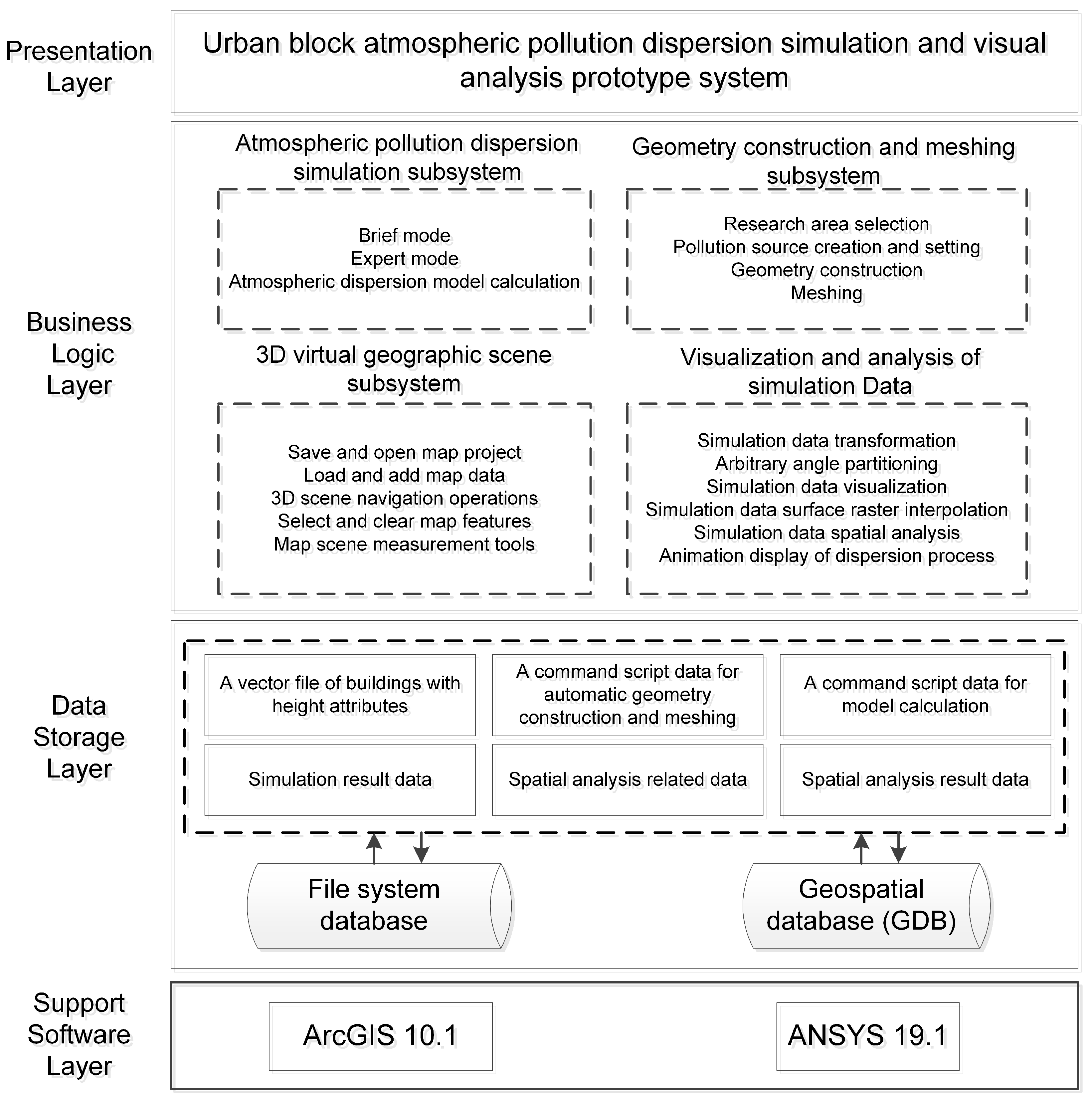
2. Methodology
2.1. Introduction of ICEM CFD and Fluent Software
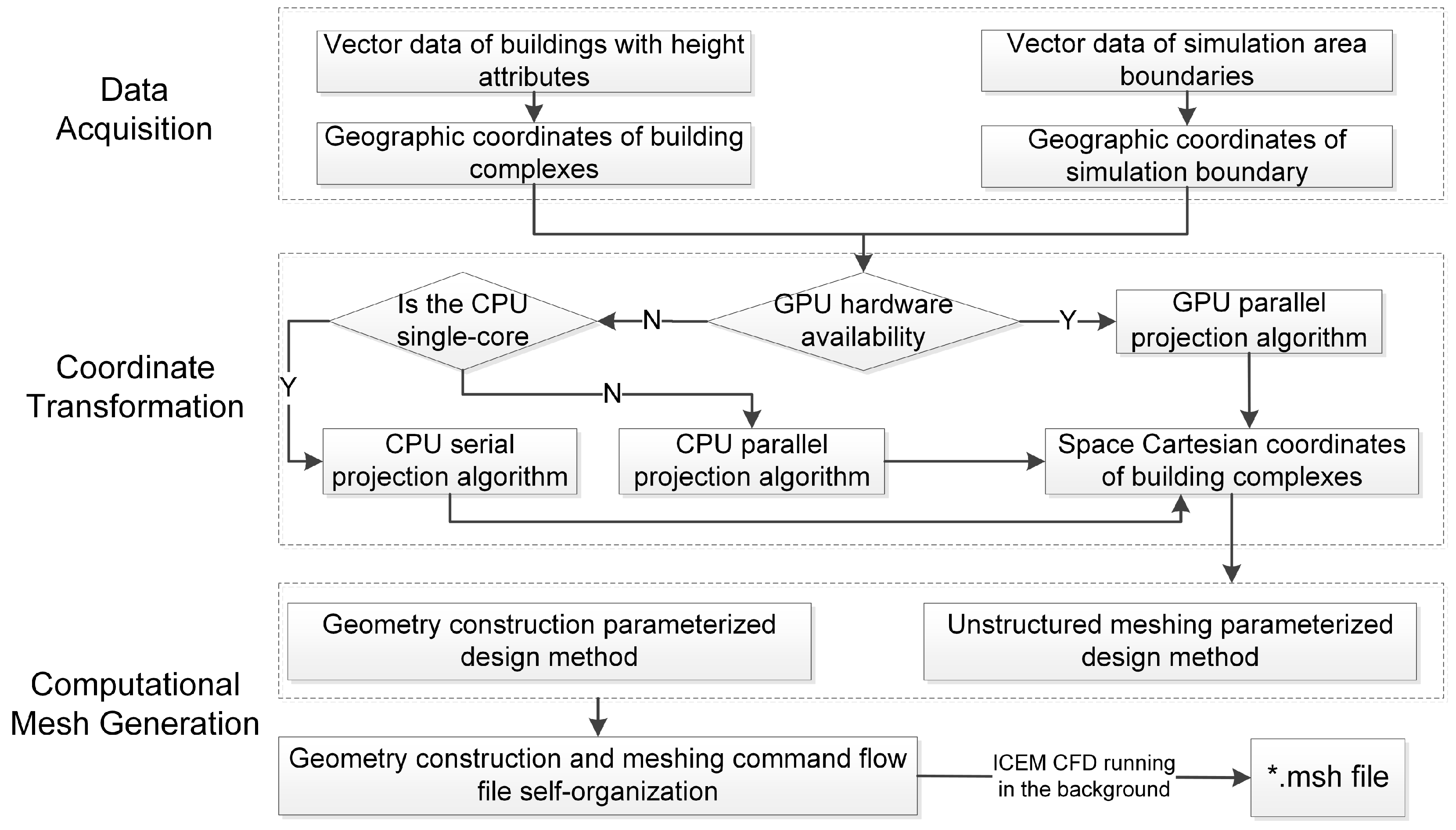
2.2. Automatic Geometry Construction and Meshing
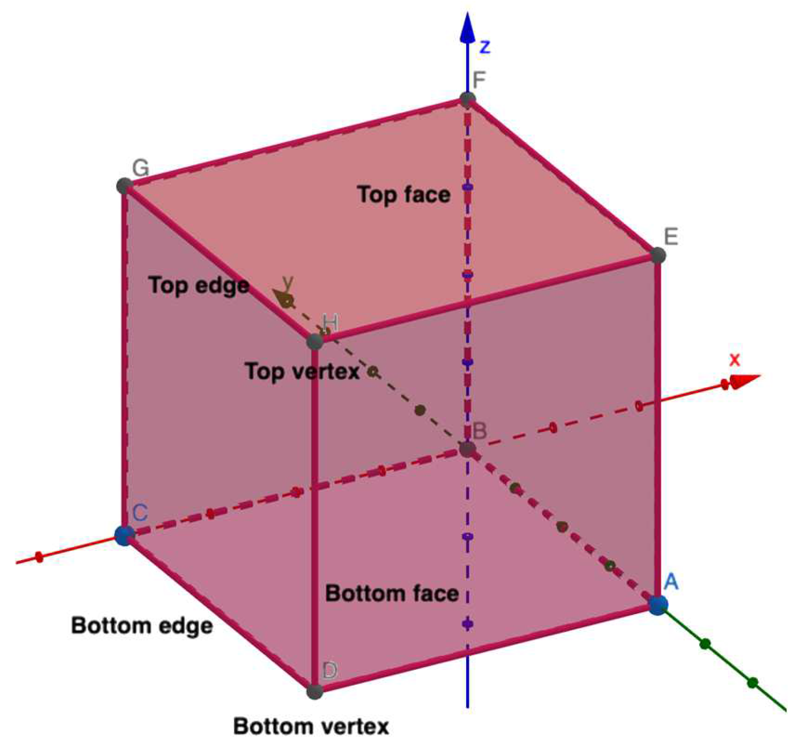
2.2.1. Extraction of Geometry Coordinates
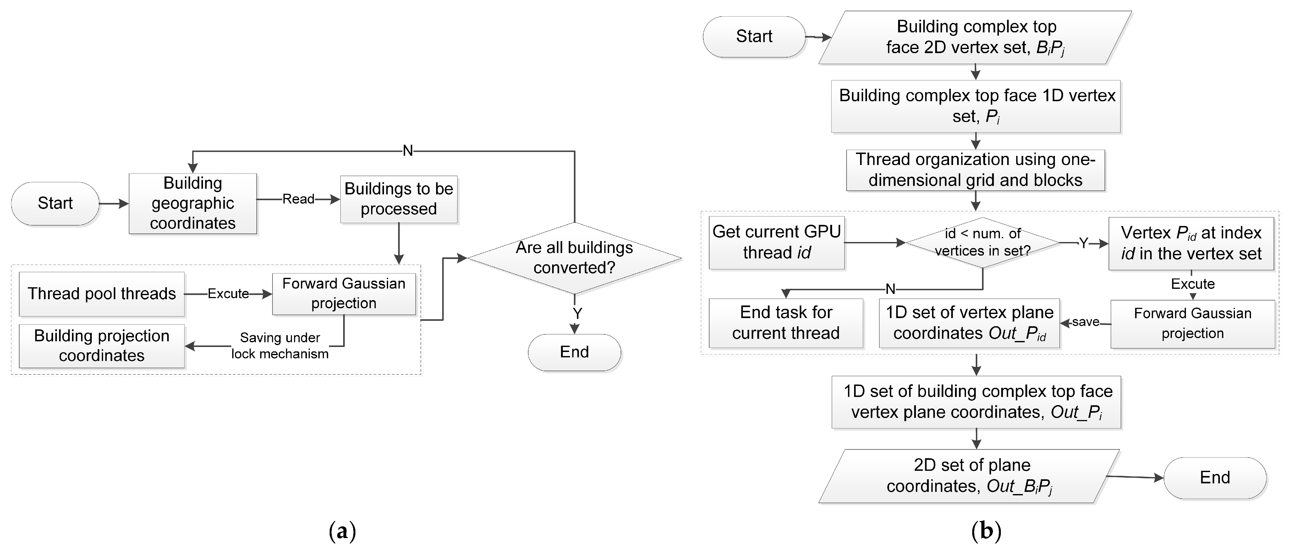
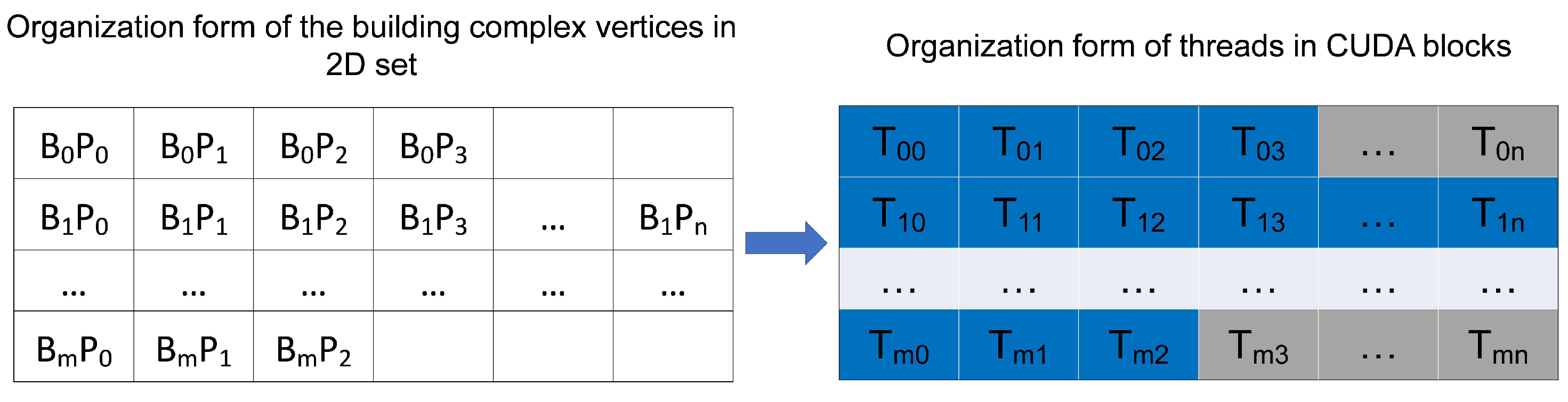
2.2.2. Parallel Approach-Based Coordinate Conversion of Building Complex
| Algorithm 1. Algorithm steps of the parallel GPU coordinate conversion of building complex vertices in CUDA-based framework. GPU parallel calculation of building vertex geographic coordinates to plane coordinates | |||
| Input: Coordinates of all building vertices λφZ_in ← {BiPj}, Number of all building vertices n | |||
| Output: Space Cartesian coordinates of all building vertices after conversion XYZ_out ← {XYZi} | |||
| 1 | function __global__ Kernel(XYZ_out, λφZ_in, n)//GPU-side functions | ||
| 2 | id ← (blockIdx.x * blockDim.x) + threadIdx.x//Get thread id | ||
| 3 | if id < n do//Perform coordinate conversion for threads that meet the condition | ||
| 4 | //Perform forward Gaussian projection | ||
| 5 | λφZ ← λφZ_in[id] | ||
| 6 | X, Y, Z = GaussianForward(λφZ) | ||
| 7 | XYZ_out[id] ← X, Y, Z//Store the converted coordinates | ||
| 8 | end if | ||
| 9 | end function | ||
| 10 | function __host__ buildsProjection(XYZ_out, λφZ_in, n)//CPU-side functions | ||
| 11 | //Apply for space on the device end | ||
| 12 | cudaMalloc(dev_λφZ_in, …), cudaMalloc(dev_ XYZ_out, …) | ||
| 13 | //Copy data from host side to device side | ||
| 14 | cudaMemcpy(dev_λφZ_in, λφZ_in, …) | ||
| 15 | cudaMemcpy(dev_XYZ_out, XYZ_out, …) | ||
| 16 | block ← blockMax/2, grid = (n − 0.5)/block + 1//Design CUDA thread organization | ||
| 17 | Kernel<<<grid,block>>>(dev_XYZ_out, dev_λφZ_in, n)//Call core functions | ||
| 18 | //Copy the calculation results from the device side back to the host side | ||
| 19 | cudaMemcpy(XYZ_out, dev_XYZ_out, …) | ||
| 20 | //Release space requested on the device side | ||
| 21 | cudaFree(dev_λφZ_in), cudaFree(dev_XYZ_out) | ||
| 22 | end function | ||
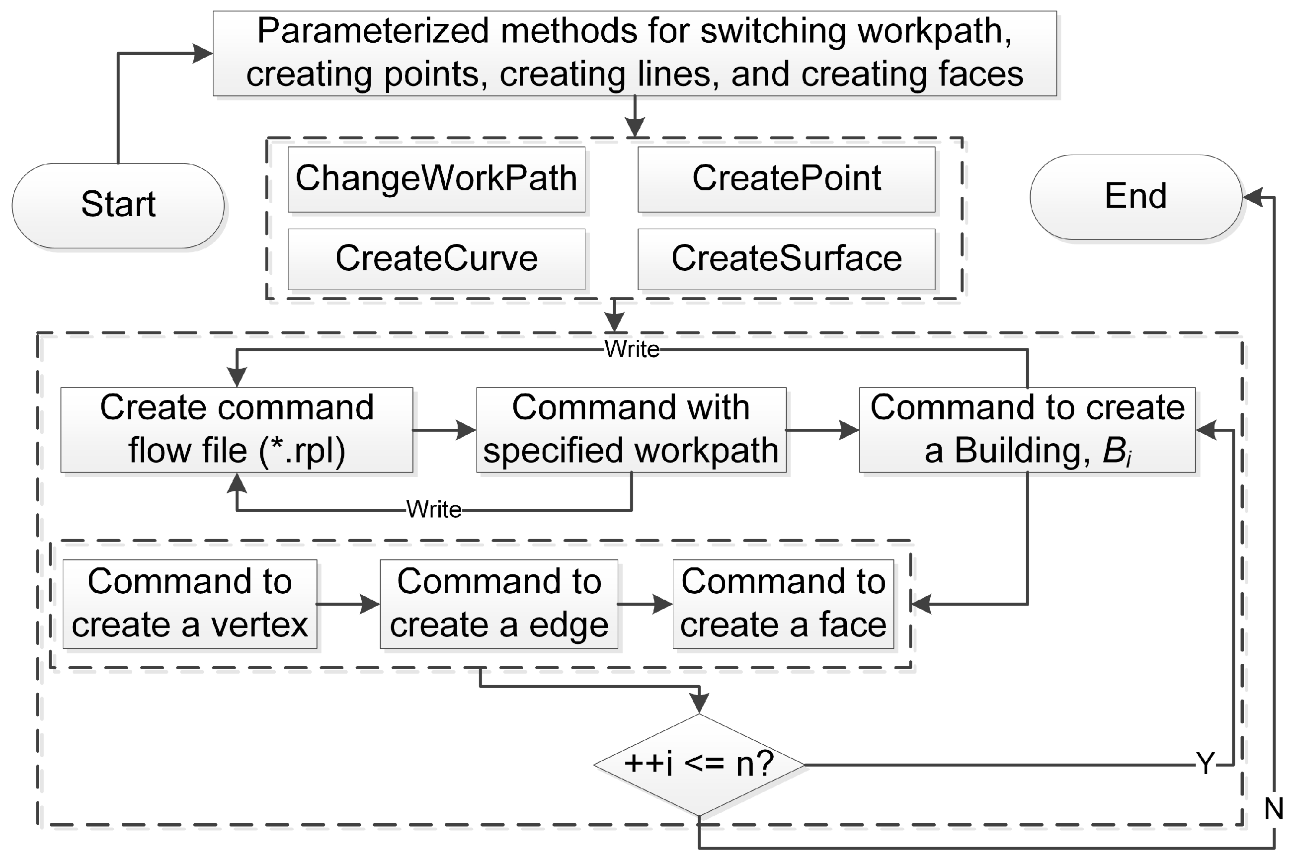
2.2.3. Parametric Design Method for Geometry Construction and Meshing
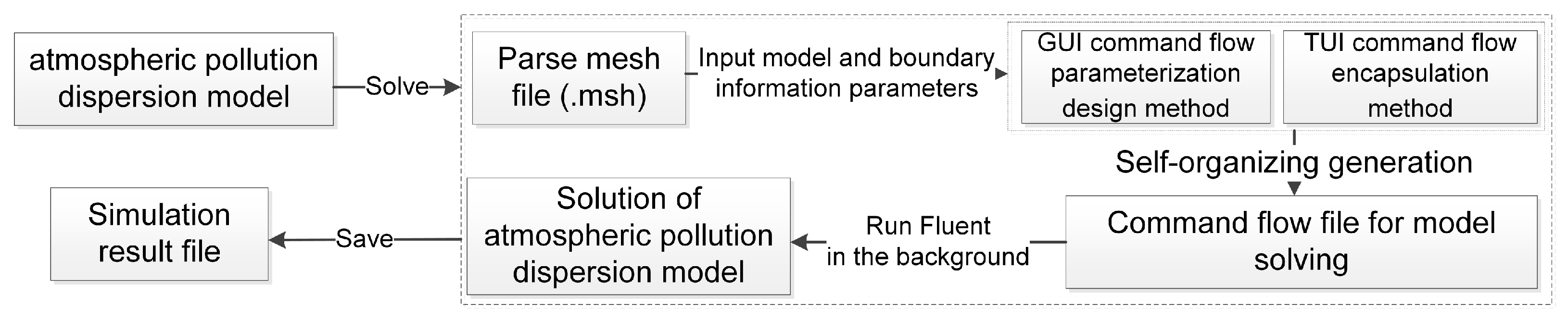
2.3. Fluent-Based Solution for Atmospheric Dispersion Models
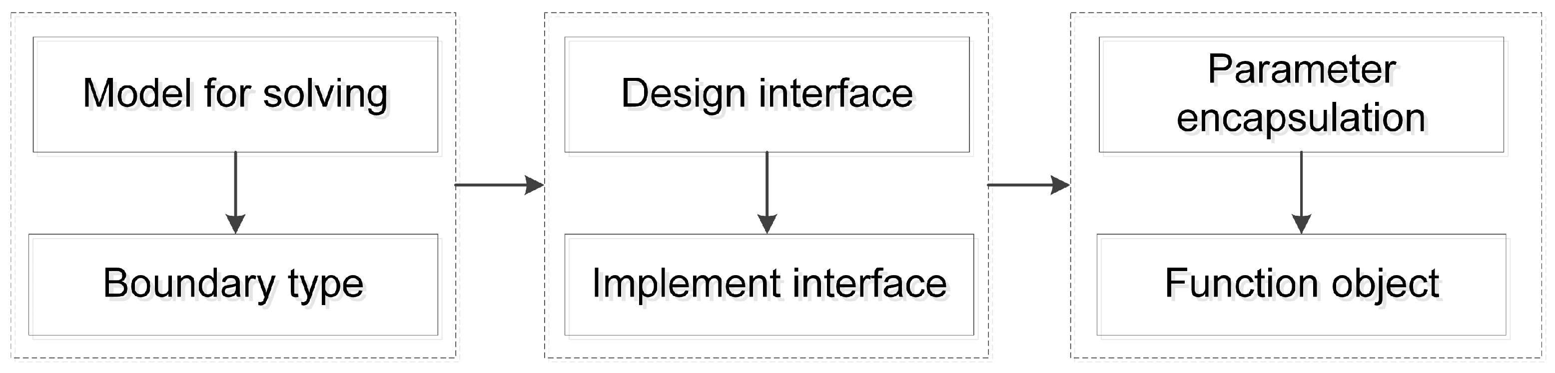
2.3.1. GUI Command Flow Parameterization Design Method
2.3.2. TUI Command Flow Encapsulation Method
2.4. Visualization and Analysis of Simulation Outputs
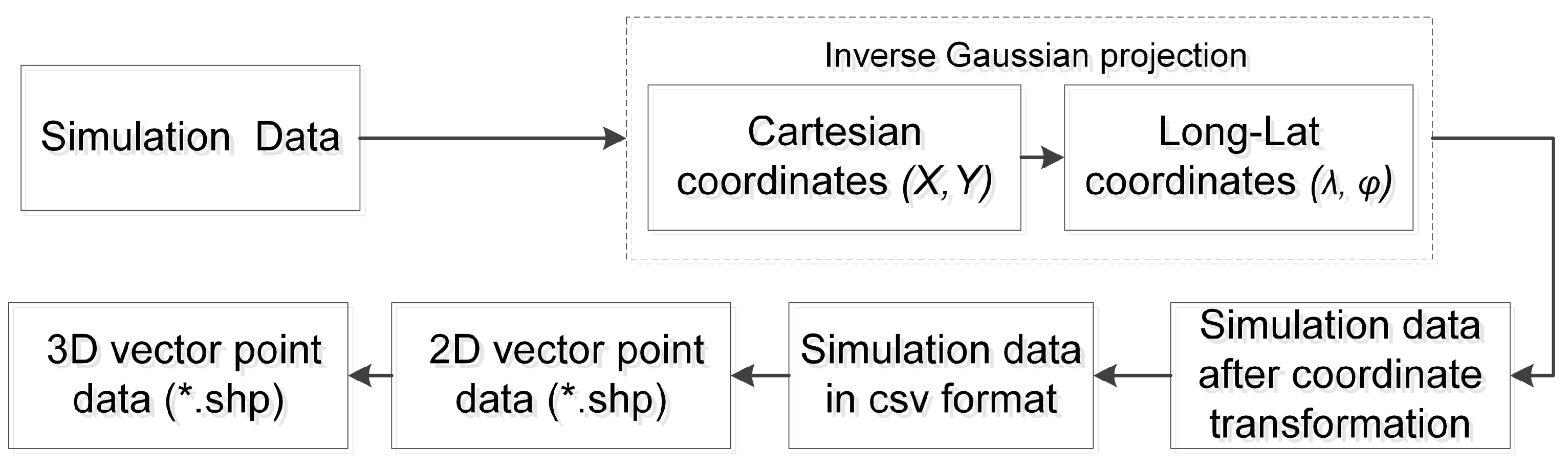
2.4.1. Conversion of Simulation Outputs to 3DGIS Data
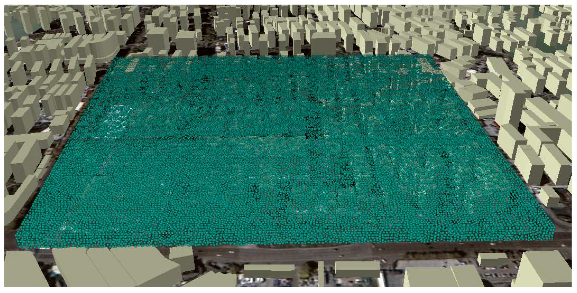
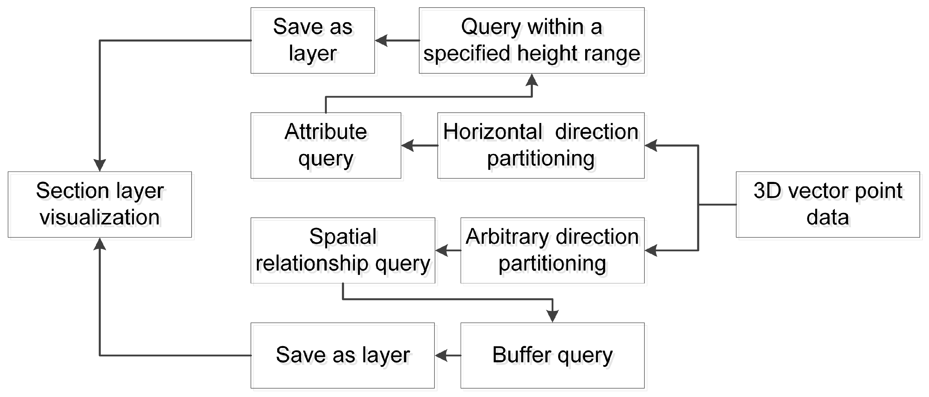
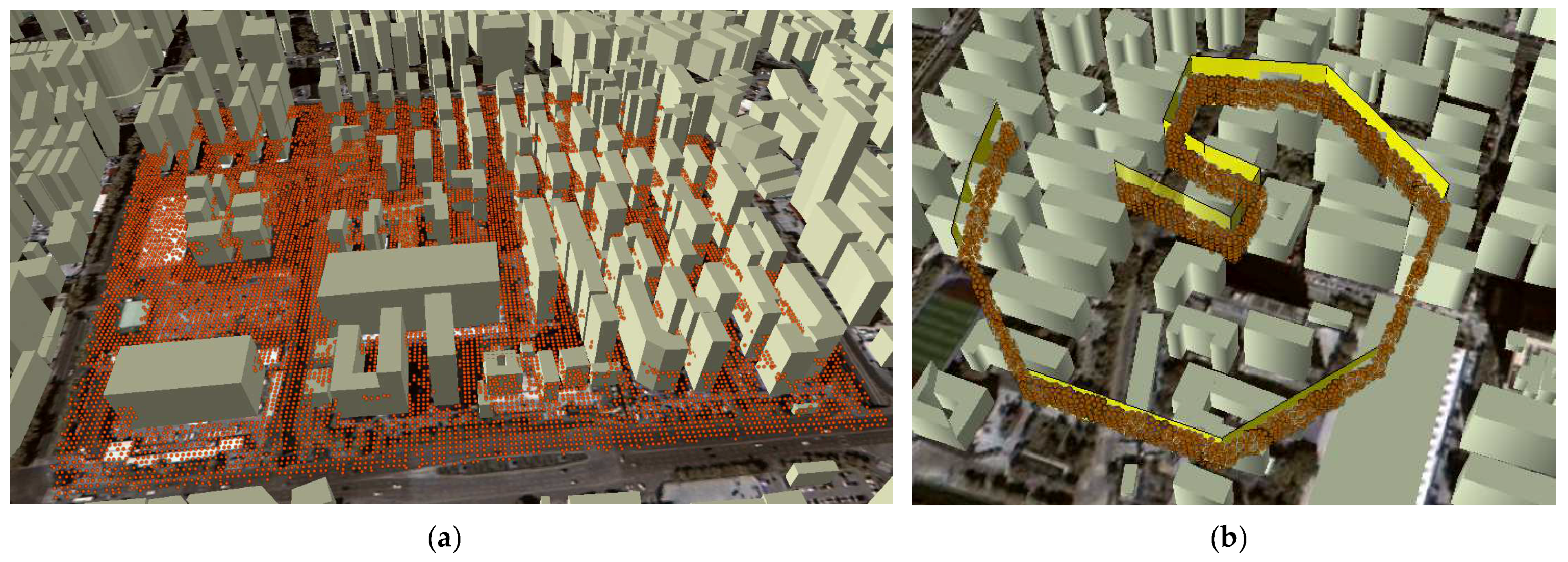
2.4.2. Multi-Angle Spatial Partitioning of Three-dimensional Spatial Simulation Outputs
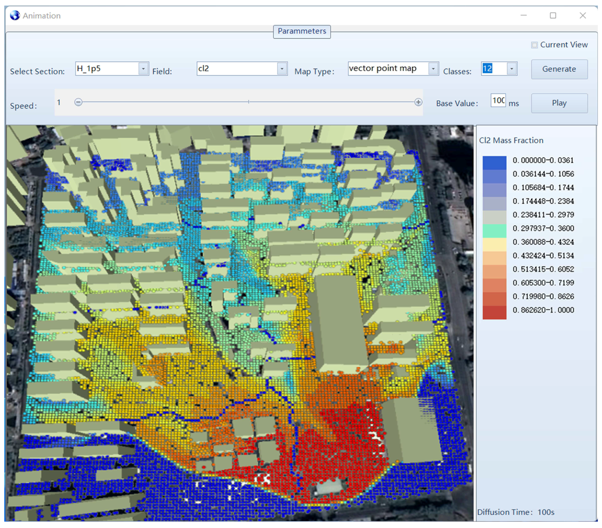
2.4.3. Spatiotemporal Multidimensional Visualization and Analysis
2.5. Implementation of the CFD Coupled with 3DGIS
3. Experiments and Results
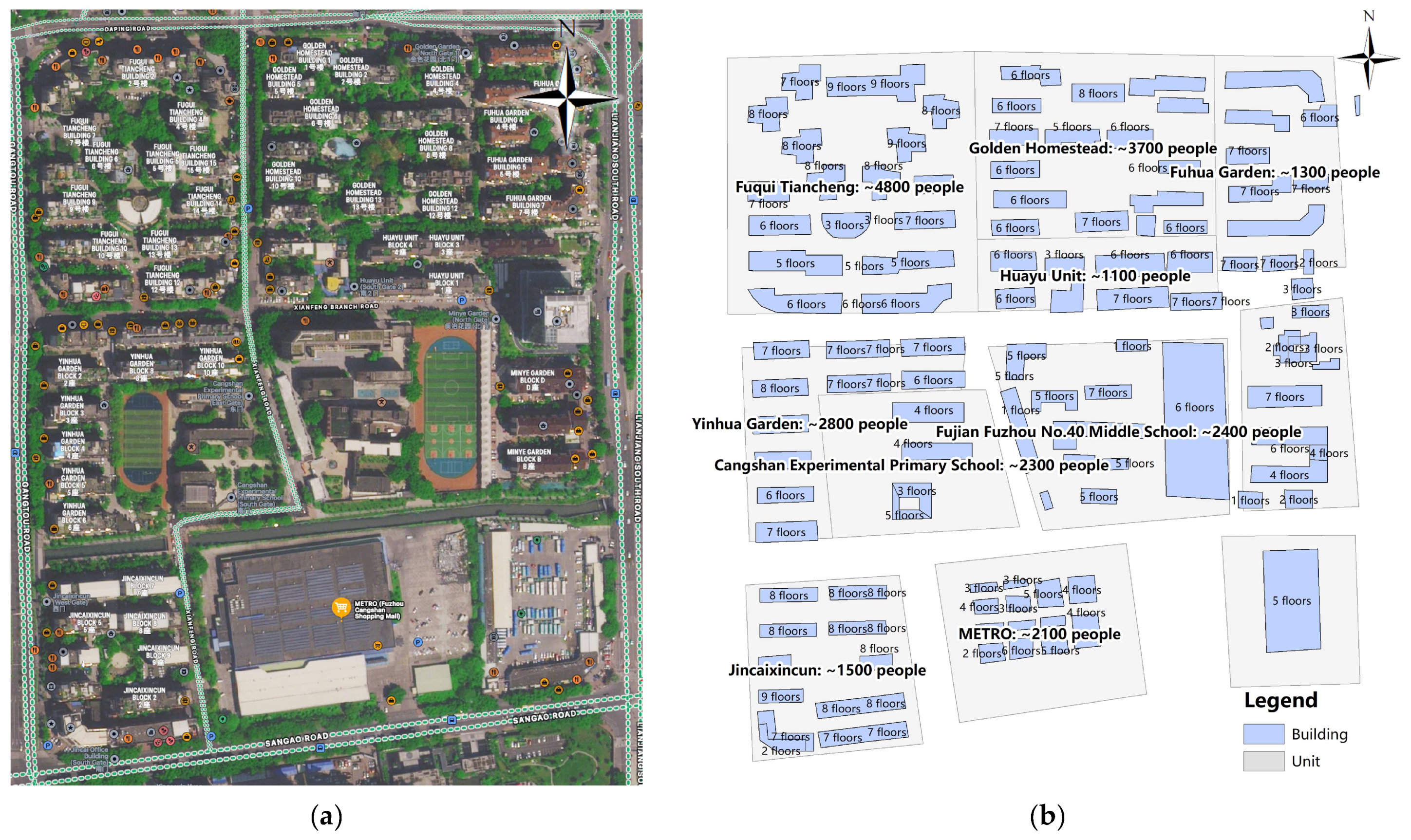
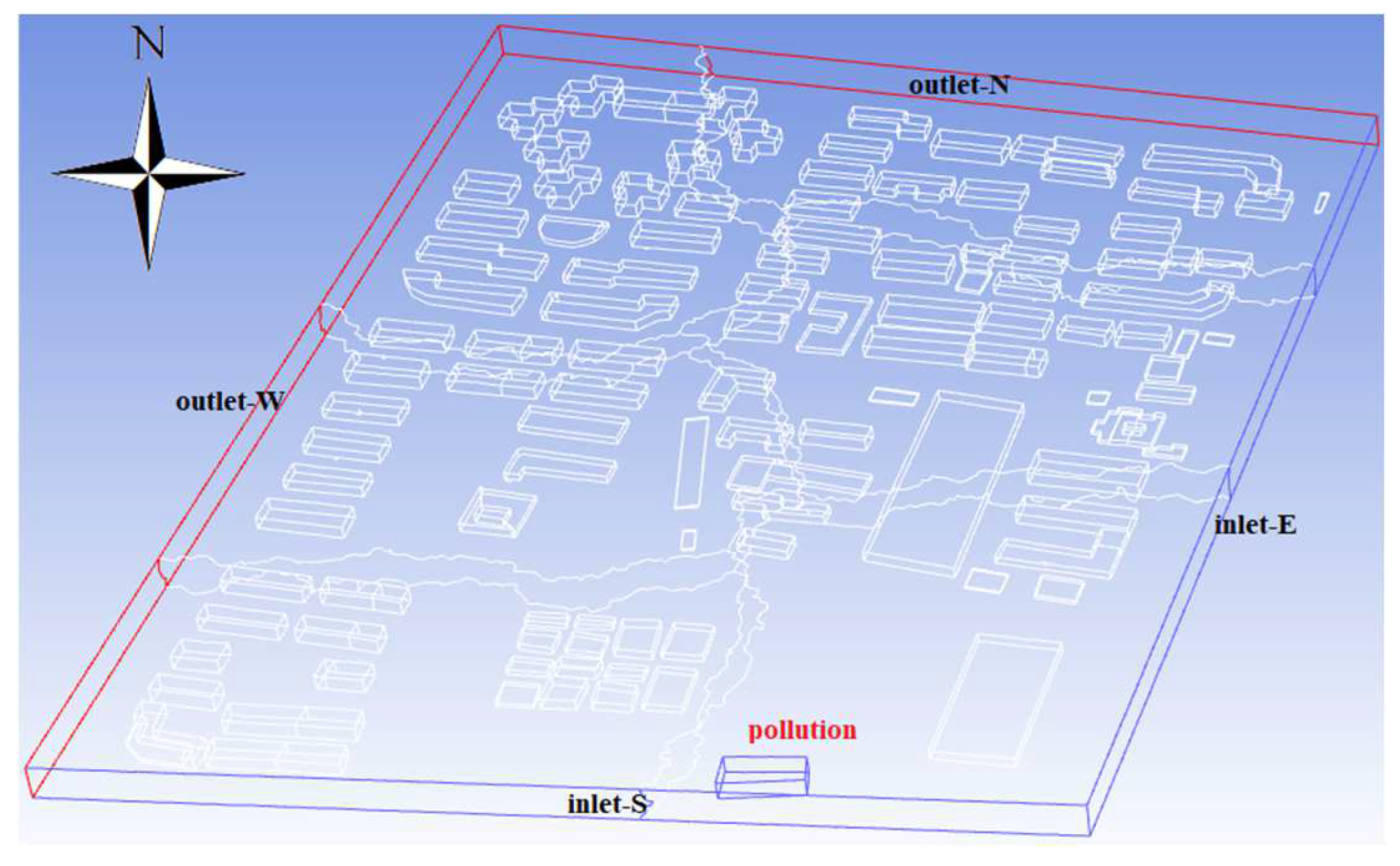
3.1. Study Area and Data
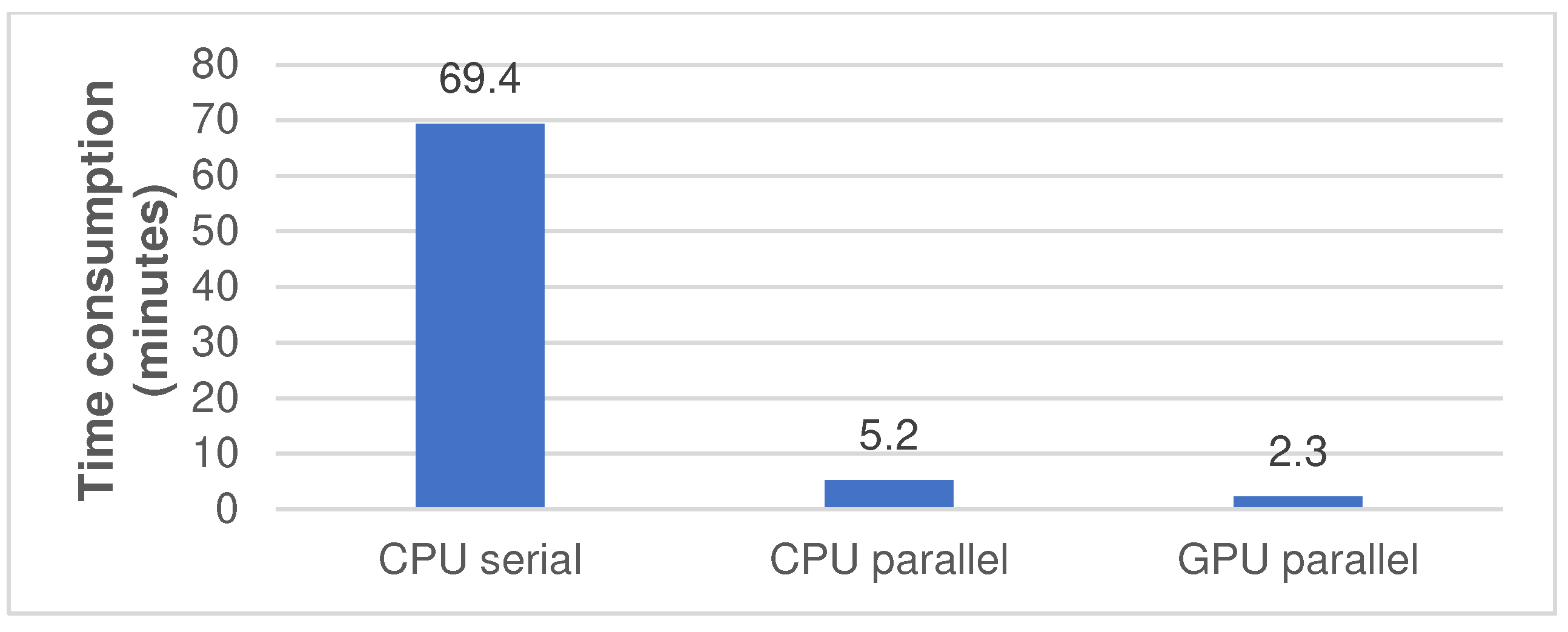
3.2. Comparison of The Efficiency of Coordinate Conversion Algorithm for Building Complex
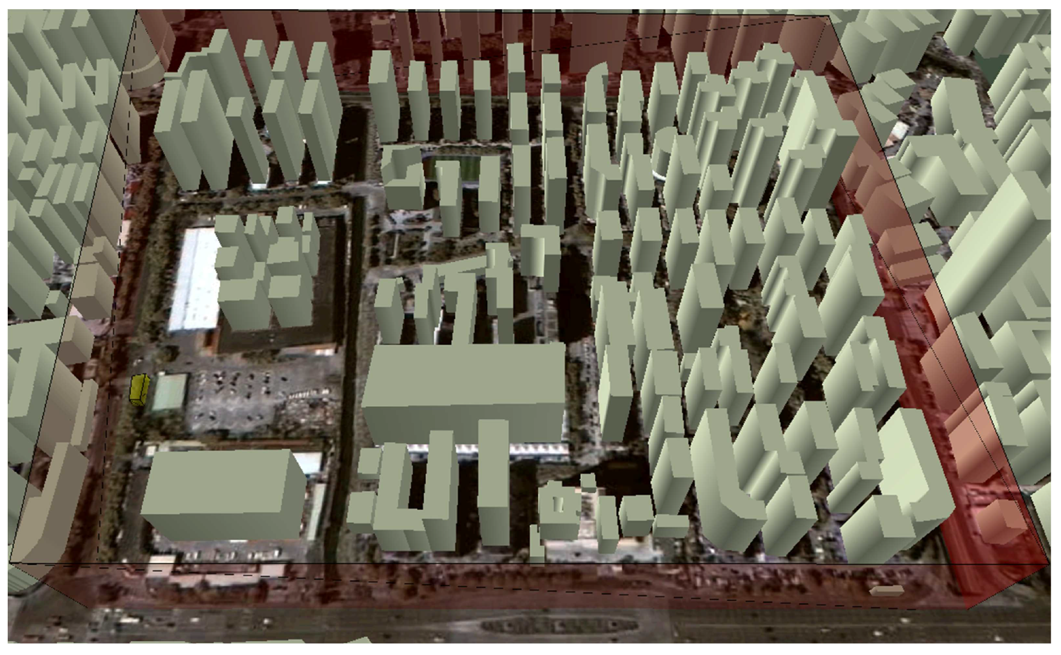
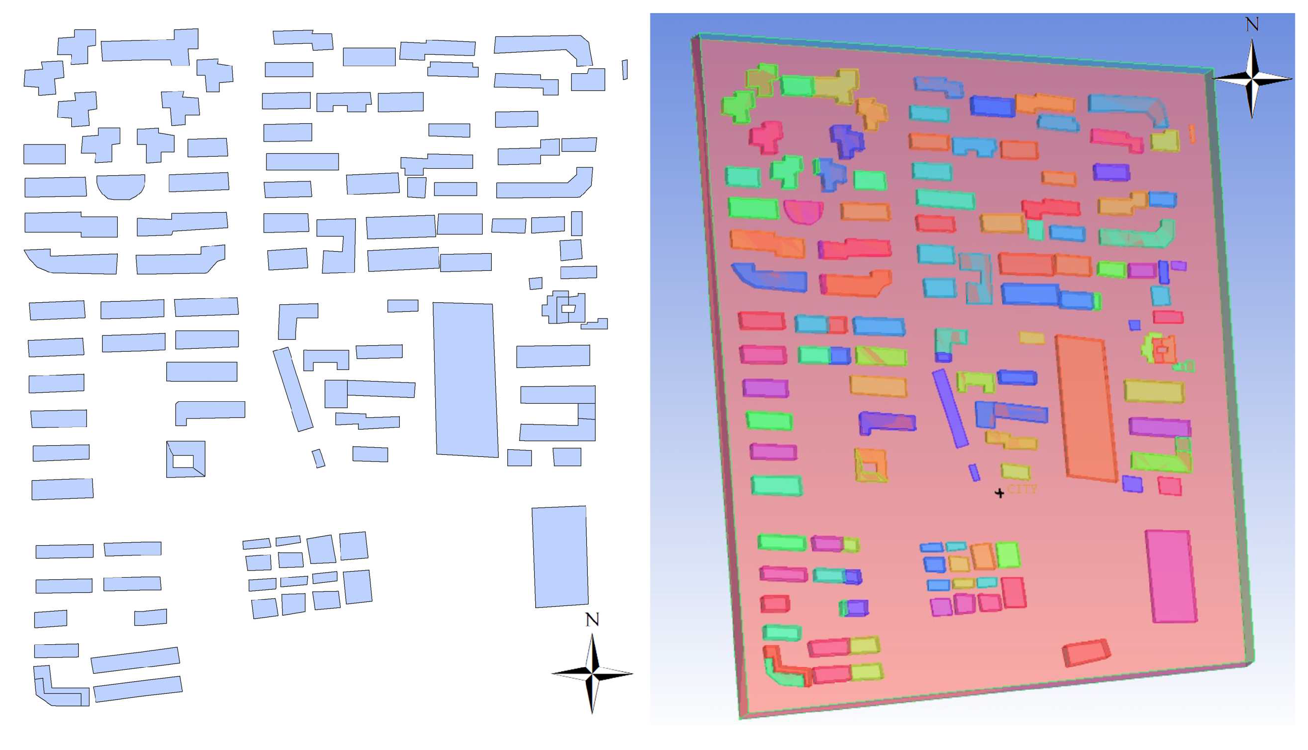
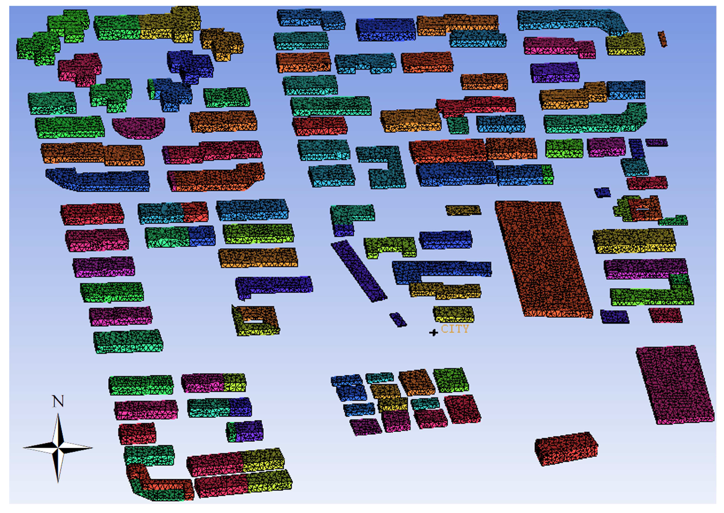
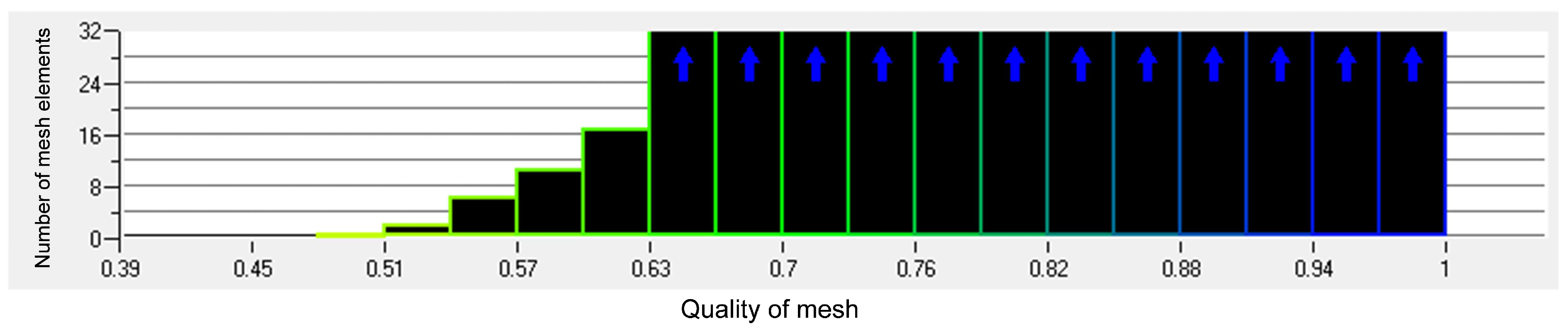
3.3. Validation of Geometry Construction and Meshing
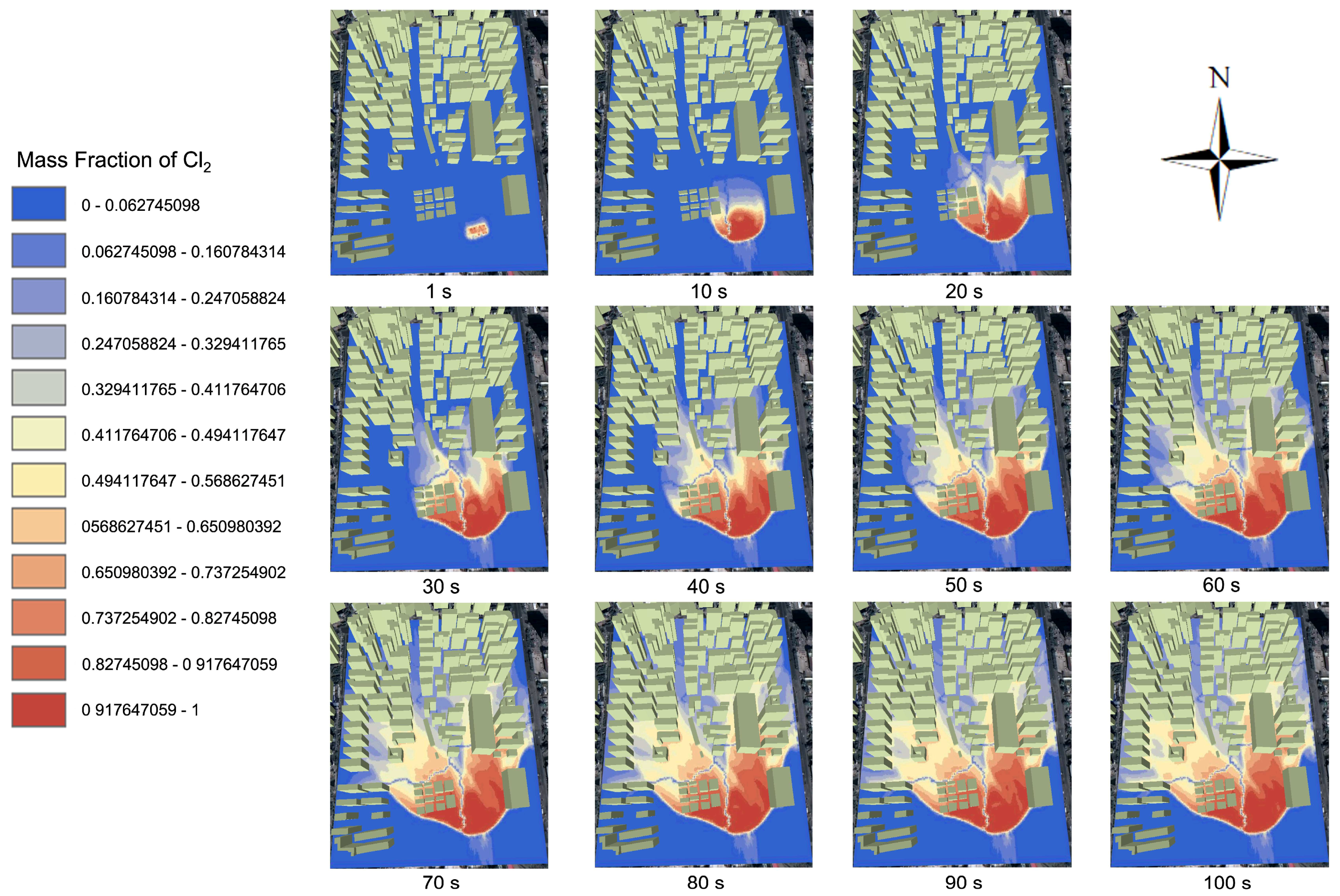
3.4. Case Study of Chlorine Dispersion Simulation
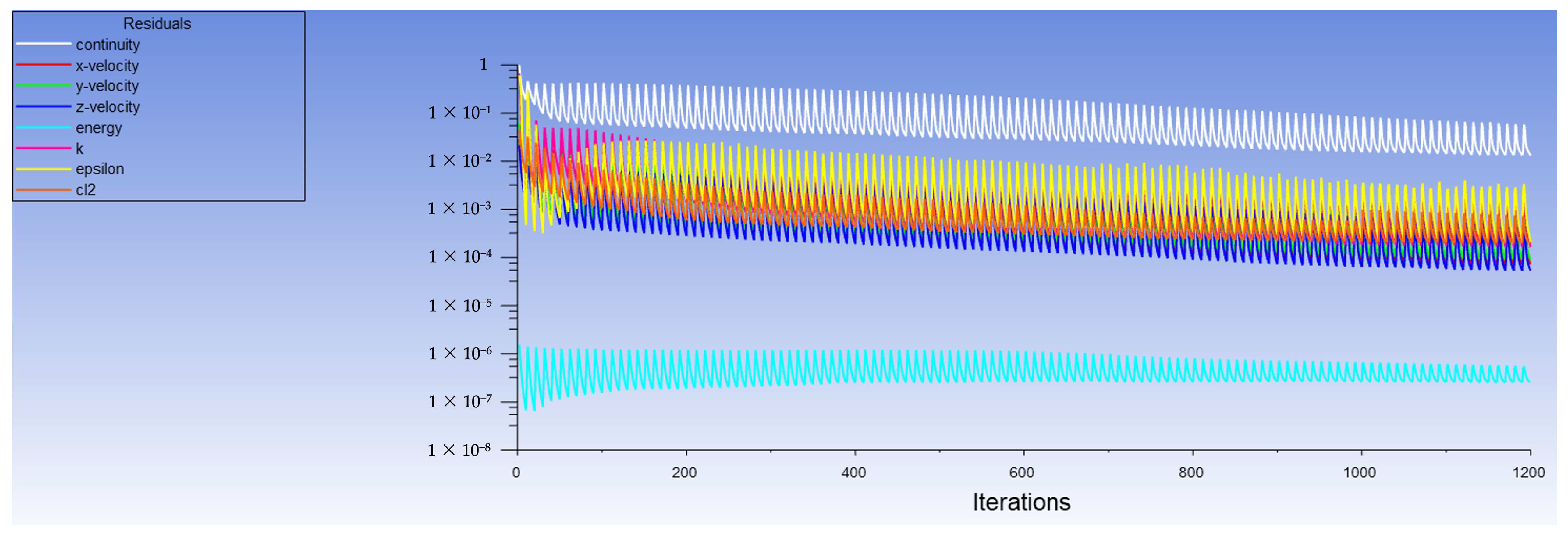
3.4.1. Simulation Parameter Setting and Model Solving
3.4.2. Analysis of Simulation Results
4. Discussion and Conclusions
- (1)
- We propose an approach for automating the construction of geometry and meshing required for CFD simulations of urban blocks. Specifically, we design both CPU and CUDA-based GPU parallel algorithms to convert building vertex coordinates in spherical coordinate systems to Cartesian coordinates in the plane quickly. We also propose using a parametric design method to encapsulate geometry construction and meshing commands to achieve automatic and rapid construction of geometry and unstructured meshing. Through experiments on the study area, we validate that the constructed geometry is correct, and the mesh quality meets the requirements with all values above 0.45. Additionally, the CPU and GPU parallel algorithms are 13.3× and 25× faster than serial, respectively.
- (2)
- We investigated CFD models related to atmospheric dispersion and proposed a parameterization design method for Fluent GUI command flow and an encapsulation method for TUI command flow, providing secondary development APIs for Fluent customization. By designing simple parameter interaction interfaces, users enabled solving CFD atmospheric dispersion models in urban blocks.
- (3)
- We propose a spatio-temporal multidimensional visualization and analysis method based on three-dimensional GIS for simulation results. Specifically, we developed a method for converting CFD simulation results into three-dimensional GIS data and achieve the coupling of CFD simulation results with three-dimensional GIS. By using three-dimensional GIS attribute and spatial topological relationship queries, we enable multi-angle spatial partitioning of simulation results. We also propose two methods for achieving spatiotemporal multidimensional visualization and animation of simulation results: layer visualization and image animation visualization.
- (4)
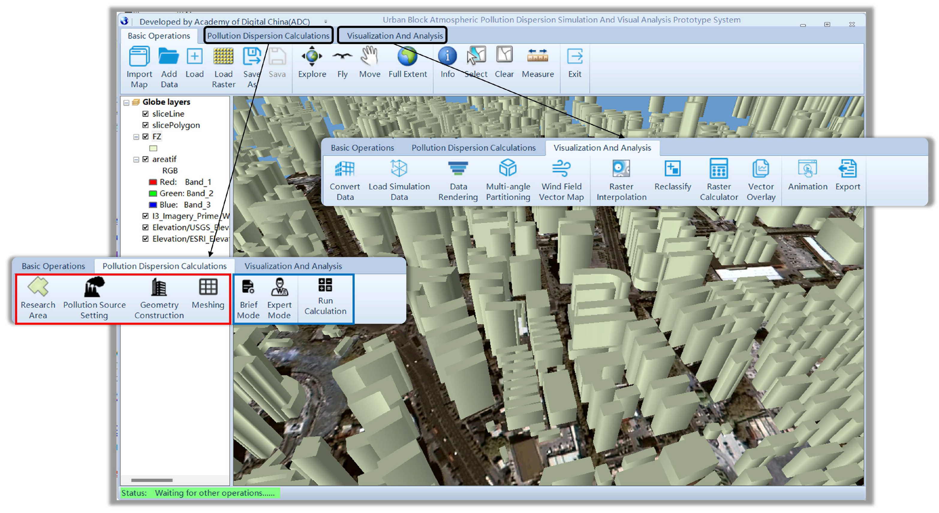
- We integrated the above-mentioned methods to develop a system coupled GIS and CFD for atmospheric pollution dispersion simulation in urban blocks. This system provides a user-friendly and easy-to-use tool for relevant departments and researchers to simulate the dispersion of atmospheric pollutants in urban areas, as well as to easily explore deep-level information.
- (1)
- The geometry is constructed only considering the buildings within the urban blocks, but not the topography, public facilities and green vegetation of the urban blocks.
- (2)
- The coupling of 3DGIS and CFD in this study is achieved through a tight integration of ArcGlobe and ANSYS software based on the .NET Framework technology framework. This involves converting GIS data into the required format for geometric construction in ICEM CFD and integrating Fluent simulation results back into GIS. All of thiese data are stored locally on the user’s computer. Consequently, our approach requires local access and conversion of shared data, which reduces efficiency and necessitates the installation of third-party software, thereby making the environment configuration complex.. In the future, open-source GIS libraries and CFD libraries can be chosen to fully integrate 3DGIS and CFD based on the method proposed in this paper.
- (3)
- For large simulation areas, the huge amount of vector point data generated by the simulation results can significantly decrease the efficiency of three-dimensional visualization, resulting in a poor user experience. In the future, it may be possible to explore the use of popular front-end two-dimensional/three-dimensional map engines, such as Cesium and Three.js, to enable three-dimensional visualization and related analysis of simulation results on the web, which could improve efficiency and user experience.
Author Contributions
Funding
Institutional Review Board Statement
Informed Consent Statement
Data Availability Statement
Conflicts of Interest
References
- Wu, C.; Wu, H.; Liu, B. Numeral Simulation of the Effects of Wind on Pipeline Natural Gas Leakage and Diffusion. Ind. Saf. Environ. Prot. 2013, 39, 46–49. [Google Scholar]
- Yang, J. Diffusion of Natural Gas Concentration Field under Humidity Gradient. Master’s Thesis, Chongqing Jiaotong University, Chongqing, China, 2014. Available online: https://kns.cnki.net/kcms2/article/abstract?v=3uoqIhG8C475KOm_zrgu4lQARvep2SAkbl4wwVeJ9RmnJRGnwiiNVnB5v6Bh-uVuVe-OXi2WINw7RONPKDGVl5QT9n3mabxH&uniplatform=NZKPT (accessed on 11 April 2023).
- Cormier, B.R.; Qi, R.; Yun, G.; Zhang, Y.; Sam Mannan, M. Application of Computational Fluid Dynamics for LNG Vapor Dispersion Modeling: A Study of Key Parameters. J. Loss Prev. Process Ind. 2009, 22, 332–352. [Google Scholar] [CrossRef]
- Tauseef, S.M.; Rashtchian, D.; Abbasi, S.A. CFD-Based Simulation of Dense Gas Dispersion in Presence of Obstacles. J. Loss Prev. Process Ind. 2011, 24, 371–376. [Google Scholar] [CrossRef]
- Yoshie, R.; Jiang, G.; Shirasawa, T.; Chung, J. CFD Simulations of Gas Dispersion around High-Rise Building in Non-Isothermal Boundary Layer. J. Wind Eng. Ind. Aerodyn. 2011, 99, 279–288. [Google Scholar] [CrossRef]
- Siddiqui, M.; Jayanti, S.; Swaminathan, T. CFD Analysis of Dense Gas Dispersion in Indoor Environment for Risk Assessment and Risk Mitigation. J. Hazard. Mater. 2012, 209–210, 177–185. [Google Scholar] [CrossRef]
- Han, G. Research on the Leakage of Buried Gas Pipeline and Diffusion Regularity. Master’s Thesis, Chongqing University, Chongqing, China, 2014. Available online: https://kns.cnki.net/kcms2/article/abstract?v=3uoqIhG8C475KOm_zrgu4lQARvep2SAkbl4wwVeJ9RmnJRGnwiiNVmSXvA452kamwJJZqoomuqhF3Ht0QXL8gR67RqjCspBj&uniplatform=NZKPT (accessed on 11 April 2023).
- Fu, J.; Xiong, X.; Li, Y.; Wei, C.; Wang, Q. Numerical Study on Leakage and Diffusion of Buried High Sulfur Natural Gas Pipelines. Contemp. Chem. Ind. 2014, 43, 1923–1926. [Google Scholar] [CrossRef]
- Feißel, T.; Büchner, F.; Kunze, M.; Rost, J.; Ivanov, V.; Augsburg, K.; Hesse, D.; Gramstat, S. Methodology for Virtual Prediction of Vehicle-Related Particle Emissions and Their Influence on Ambient PM10 in an Urban Environment. Atmosphere 2022, 13, 1924. [Google Scholar] [CrossRef]
- Schalau, S.; Habib, A.; Michel, S. A Modified K-ε Turbulence Model for Heavy Gas Dispersion in Built-Up Environment. Atmosphere 2023, 14, 161. [Google Scholar] [CrossRef]
- Sabatino, S.D.; Buccolieri, R.; Pulvirenti, B.; Britter, R.E. Flow and Pollutant Dispersion in Street Canyons Using FLUENT and ADMS-Urban. Environ. Model. Assess. 2008, 13, 369–381. [Google Scholar] [CrossRef]
- Toja-Silva, F.; Chen, J.; Hachinger, S.; Hase, F. CFD Simulation of CO2 Dispersion from Urban Thermal Power Plant: Analysis of Turbulent Schmidt Number and Comparison with Gaussian Plume Model and Measurements. J. Wind Eng. Ind. Aerodyn. 2017, 169, 177–193. [Google Scholar] [CrossRef]
- Yuan, X.; Chen, C.; Lei, X.; Yuan, Y.; Muhammad Adnan, R. Monthly Runoff Forecasting Based on LSTM–ALO Model. Stoch. Environ. Res. Risk Assess. 2018, 32, 2199–2212. [Google Scholar] [CrossRef]
- Adnan, R.M.; Mostafa, R.R.; Elbeltagi, A.; Yaseen, Z.M.; Shahid, S.; Kisi, O. Development of New Machine Learning Model for Streamflow Prediction: Case Studies in Pakistan. Stoch. Environ. Res. Risk Assess. 2022, 36, 999–1033. [Google Scholar] [CrossRef]
- Adnan, R.M.; Mostafa, R.; Kisi, O.; Yaseen, Z.M.; Shahid, S.; Zounemat-Kermani, M. Improving Streamflow Prediction Using a New Hybrid ELM Model Combined with Hybrid Particle Swarm Optimization and Grey Wolf Optimization. Knowl. -Based Syst. 2021, 230, 107379. [Google Scholar] [CrossRef]
- Adnan, R.M.; Kisi, O.; Mostafa, R.R.; Ahmed, A.N.; El-Shafie, A. The Potential of a Novel Support Vector Machine Trained with Modified Mayfly Optimization Algorithm for Streamflow Prediction. Hydrol. Sci. J. 2022, 67, 161–174. [Google Scholar] [CrossRef]
- Ikram, R.M.A.; Ewees, A.A.; Parmar, K.S.; Yaseen, Z.M.; Shahid, S.; Kisi, O. The Viability of Extended Marine Predators Algorithm-Based Artificial Neural Networks for Streamflow Prediction. Appl. Soft Comput. 2022, 131, 109739. [Google Scholar] [CrossRef]
- Wu, Q.; Lin, H. A Novel Optimal-Hybrid Model for Daily Air Quality Index Prediction Considering Air Pollutant Factors. Sci. Total Environ. 2019, 683, 808–821. [Google Scholar] [CrossRef]
- Li, X.; Luo, A.; Li, J.; Li, Y. Air Pollutant Concentration Forecast Based on Support Vector Regression and Quantum-Behaved Particle Swarm Optimization. Environ. Model. Assess. 2019, 24, 205–222. [Google Scholar] [CrossRef]
- Niu, M.; Zhang, Y.; Ren, Z. Deep Learning-Based PM2.5 Long Time-Series Prediction by Fusing Multisource Data—A Case Study of Beijing. Atmosphere 2023, 14, 340. [Google Scholar] [CrossRef]
- Ong, B.T.; Sugiura, K.; Zettsu, K. Dynamically Pre-Trained Deep Recurrent Neural Networks Using Environmental Monitoring Data for Predicting PM2.5. Neural Comput. Appl. 2016, 27, 1553–1566. [Google Scholar] [CrossRef]
- Esager, M.W.M.; Ünlü, K.D. Forecasting Air Quality in Tripoli: An Evaluation of Deep Learning Models for Hourly PM2.5 Surface Mass Concentrations. Atmosphere 2023, 14, 478. [Google Scholar] [CrossRef]
- Zhang, Z.; Ren, J.; Chang, Y. Improving Intra-Urban Prediction of Atmospheric Fine Particles Using a Hybrid Deep Learning Approach. Atmosphere 2023, 14, 599. [Google Scholar] [CrossRef]
- Li, X.; Peng, L.; Yao, X.; Cui, S.; Hu, Y.; You, C.; Chi, T. Long Short-Term Memory Neural Network for Air Pollutant Concentration Predictions: Method Development and Evaluation. Environ. Pollut. 2017, 231, 997–1004. [Google Scholar] [CrossRef]
- Kuremoto, T.; Kimura, S.; Kobayashi, K.; Obayashi, M. Time Series Forecasting Using a Deep Belief Network with Restricted Boltzmann Machines. Neurocomputing 2014, 137, 47–56. [Google Scholar] [CrossRef]
- Wang, B.; Qian, F. Three Dimensional Gas Dispersion Modeling Using Cellular Automata and Artificial Neural Network in Urban Environment. Process Saf. Environ. Prot. 2018, 120, 286–301. [Google Scholar] [CrossRef]
- Huang, C.-J.; Kuo, P.-H. A Deep CNN-LSTM Model for Particulate Matter (PM2.5) Forecasting in Smart Cities. Sensors 2018, 18, 2220. [Google Scholar] [CrossRef]
- Pak, U.; Kim, C.; Ryu, U.; Sok, K.; Pak, S. A Hybrid Model Based on Convolutional Neural Networks and Long Short-Term Memory for Ozone Concentration Prediction. Air Qual. Atmosphere Health 2018, 11, 883–895. [Google Scholar] [CrossRef]
- Cao, D. The Secondary Development of Fluent and Research and Application in Computer-Aided Optimization and Design of Pump about It. Master’s Thesis, North China Electric Power University, Beijing, China, 2002. Available online: https://kns.cnki.net/kcms2/article/abstract?v=3uoqIhG8C475KOm_zrgu4m9eu-VXu9H75RhMZCEMue9h8LplqMYx9zGVlbBb7nVMKWq_bvhtNu58msc-qJ3_mXCXmN6p2uBD&uniplatform=NZKPT (accessed on 11 April 2023).
- Zhang, Z.; Gao, B.; Zheng, C.; Wang, Y. Analysis of Transient Pressure Induced by High-Speed Train Passing a Tunnel Based on the Second Development of Fluent. J. Railw. Eng. Soc. 2005, 41–44, 54. [Google Scholar]
- Li, H.; Bi, X.; Huang, X.; Suo, W. Shape Parametric Constructing Model of Radiator Core Based on the Secondary Development of Fluent. Veh. Power Technol. 2008, 36–39, 43. [Google Scholar] [CrossRef]
- Li, H.; Wang, G.; Wang, D.; Tan, B. Journal File of the Secondary Development of the Fluent Based on the Ventilating System of the Subway. Comput. Syst. Appl. 2015, 24, 233–238. [Google Scholar]
- Xiao, H.; Gao, C.; Dang, Y.; Yang, Y.; Wang, G. Secondary Development of FLUENT and Application in Numerical Simulation of Aerodynamic Characteristics for Rockets. Aeronaut. Comput. Tech. 2009, 39, 55–57. [Google Scholar]
- Li, X.; Lu, J.; Tan, S.; Li, K.; Du, P. Simulation on Moving Magnetic Field of Electromagnetic Rail launch Based on Fluent Secondary Development. Proc. CSEE 2020, 40, 6364–6371. [Google Scholar] [CrossRef]
- Murakami, S. Environmental Design of Outdoor Climate Based on CFD. Fluid Dyn. Res. 2006, 38, 108–126. [Google Scholar] [CrossRef]
- Chu, A.K.M.; Kwok, R.C.W.; Yu, K.N. Study of Pollution Dispersion in Urban Areas Using Computational Fluid Dynamics (CFD) and Geographic Information System (GIS). Environ. Model. Softw. 2005, 20, 273–277. [Google Scholar] [CrossRef]
- Coirier, W.J.; Kim, S. CFD Modeling for Urban Area Contaminant Transport and Dispersion: Model Description and Data Requirements. In Proceedings of the Sixth Symposium on the Urban Environment, The 86th AMS Annual Meeting, Atlanta, GA, USA, 2 February 2006. [Google Scholar]
- Wong, D.W.; Camelli, F.; Sonwalkar, M. Integrating Computational Fluid Dynamics (CFD) Models with GIS: An Evaluation on Data Conversion Formats. In Geoinformatics 2007: Geospatial Information Science; SPIE: Bellingham, WA, USA, 2007; Volume 6753, pp. 368–378. [Google Scholar] [CrossRef]
- van Hooff, T.; Blocken, B. Coupled Urban Wind Flow and Indoor Natural Ventilation Modelling on a High-Resolution Grid: A Case Study for the Amsterdam ArenA Stadium. Environ. Model. Softw. 2010, 25, 51–65. [Google Scholar] [CrossRef]
- Zheng, M.; Jin, M.; Guo, f. Modeling and Simulation of Toxic Gas Dispersion in Urban Streets Supported by GIS. Geomat. Inf. Sci. Wuhan Univ. 2013, 38, 935–939. [Google Scholar] [CrossRef]
- Xu, Y. Application Research of Atmospheric Pollution in the City Coupled with CFD Software and Geographic Information System (GIS). Master’s Thesis, Chongqing Jiaotong University, Chongqing, China, 2014. Available online: https://kns.cnki.net/kcms2/article/abstract?v=3uoqIhG8C475KOm_zrgu4lQARvep2SAkbl4wwVeJ9RmnJRGnwiiNVoWUqW9aqtc51NN9UurKIfZzT152-rm_NjKmlPFLP6yC&uniplatform=NZKPT (accessed on 8 March 2023).
- Jiao, X. Application Research of Pollutant Diffusion of Traffic in the City Coupled with CFD Software and Geographic Information System(GIS). Master’s Thesis, Chongqing Jiaotong University, Chongqing, China, 2016. Available online: https://kns.cnki.net/kcms2/article/abstract?v=3uoqIhG8C475KOm_zrgu4lQARvep2SAkkyu7xrzFWukWIylgpWWcEoXyvc0-RZfX-EKX-ZhSaLva1axFC5O_ABrlQpUWkqcN&uniplatform=NZKPT (accessed on 8 March 2023).
- Chang, S.; Jiang, Q.; Zhao, Y. Integrating CFD and GIS into the Development of Urban Ventilation Corridors: A Case Study in Changchun City, China. Sustainability 2018, 10, 1814. [Google Scholar] [CrossRef]
- Wang, W.; Chen, H.; Wang, X.; Du, S.; Xv, T. Application of GIS and CFD Software in Sind Farm. Hydropower New Energy 2020, 34, 29–32. [Google Scholar] [CrossRef]
- Wu, Q.; Huang, J.; Sheng, L.; Tan, S.; Wang, Q.; Sun, Z. Spatio-temporal and Multi-dimensional Visualizations for the Simulation Result of CALPUFF Model. J. Geo-Inf. Sci. 2015, 17, 206–214. [Google Scholar]
- Wu, Q.; Tang, S.; Huang, J. A GeoJSON-based mobile visualization method for emergency air pollution simulation disaster condition. J. Nat. Disasters 2015, 24, 165–171. [Google Scholar] [CrossRef]


| Operations | Commands |
|---|---|
| setting the global meshing parameters | ic_set_meshing_params global |
| setting geometric parameters for a specific geometry family | ic_geo_set_family_params |
| generating a tetrahedral mesh | ic_run_tetra |
| smoothing the mesh elements | ic_smooth_elements |
| saving the generated unstructured mesh | ic_save_unstruct |
| executing a user-defined script or external program | ic_exec |
| Directory Name | Functional Descriptions |
|---|---|
| adapt/ | contains commands related to mesh adaptation |
| adjoint/ | contains commands related to adjoint solver |
| define/ | contains commands to define materials, boundary conditions, and other simulation parameters |
| display/ | contains commands to control the display of the Fluent GUI |
| file/ | contains commands to import or export files |
| mesh/ | contains commands related to mesh generation and manipulation |
| parallel/ | contains commands related to parallel |
| plot/ | contains commands to create plots and animations |
| report/ | contains commands to generate reports, such as force or mass reports |
| server/ | contains commands to control the Fluent server |
| solve/ | contains commands related to the solution of the fluid problem |
| surface/ | contains commands related to surface modeling |
| turbo/ | contains commands related to turbomachinery simulation |
| views/ | contains commands to create, save, and restore views of the Fluent GUI |
| Parameter | CPU | GPU |
|---|---|---|
| Model | Intel(R) Xeon(R) Gold 5228 | NVIDIA GeForce RTX 2080 Ti |
| Other properties | Number of cores: 24; Number of logical processors: 48; L1 cache: 1.5 MB; L2 cache: 24.0 MB; L3 cache: 33.0 MB | Maximum number of blocks in each dimension of the grid: 2,147,483,647, 65,535, 65,535; Maximum number of threads in each dimension of a block: 1024, 1024, 64 |
| Zona Name | Type | Boundary Conditions |
|---|---|---|
| Pollution truck | mass-flow-inlet | Mass Flow Method: Mass Flux; Reference Frame: Absolute; Mass Flux: 6 kg/(m2-s); Initial Gauge Pressure: 0; Direction method: Normal to Boundary; Temperature: 300 k |
| inlet-S, inlet-E | velocity-inlet | Velocity Method: Magnitude, Normal to boundary; Reference Frame: Absolute; Initial gauge Pressure: 0; Temperature: 300 k |
| outlet-W, outlet-N | outflow | Flow Rate Weighting: 1 |
| top and bottom surface, building | wall | Wall Motion: Stationary; Shear Condition: No Slip; Roughness Models: Standard; Temperature: 300 k |
Disclaimer/Publisher’s Note: The statements, opinions and data contained in all publications are solely those of the individual author(s) and contributor(s) and not of MDPI and/or the editor(s). MDPI and/or the editor(s) disclaim responsibility for any injury to people or property resulting from any ideas, methods, instructions or products referred to in the content. |
© 2023 by the authors. Licensee MDPI, Basel, Switzerland. This article is an open access article distributed under the terms and conditions of the Creative Commons Attribution (CC BY) license (https://creativecommons.org/licenses/by/4.0/).
Share and Cite
Wu, Q.; Wang, Y.; Sun, H.; Lin, H.; Zhao, Z. A System Coupled GIS and CFD for Atmospheric Pollution Dispersion Simulation in Urban Blocks. Atmosphere 2023, 14, 832. https://doi.org/10.3390/atmos14050832
Wu Q, Wang Y, Sun H, Lin H, Zhao Z. A System Coupled GIS and CFD for Atmospheric Pollution Dispersion Simulation in Urban Blocks. Atmosphere. 2023; 14(5):832. https://doi.org/10.3390/atmos14050832
Chicago/Turabian StyleWu, Qunyong, Yuhang Wang, Haoyu Sun, Han Lin, and Zhiyuan Zhao. 2023. "A System Coupled GIS and CFD for Atmospheric Pollution Dispersion Simulation in Urban Blocks" Atmosphere 14, no. 5: 832. https://doi.org/10.3390/atmos14050832