Article

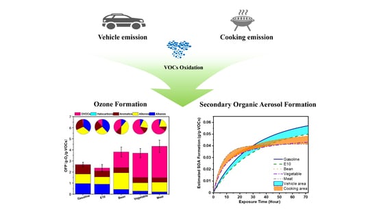
Characteristics and Secondary Organic Aerosol Formation of Volatile Organic Compounds from Vehicle and Cooking Emissions

1
State Key Joint Laboratory of Environmental Simulation and Pollution Control, International Joint Laboratory for Regional Pollution Control, Ministry of Education (IJRC), College of Environmental Sciences and Engineering, Peking University, Beijing 100871, China
2
Collaborative Innovation Center of Atmospheric Environment and Equipment Technology, Nanjing University of Information Science & Technology, Nanjing 210044, China
3
Institute of Energy and Climate Research, Troposphere (IEK-8), Forschungszentrum Jülich GmbH, 52428 Jülich, Germany
4
School of Energy and Power Engineering, University of Shanghai for Science and Technology, Shanghai 200093, China
5
State Key Laboratory of Automotive Safety and Energy, Tsinghua University, Beijing 100871, China
6
State Key Laboratory of Multiphase Complex Systems, Institute of Process Engineering, Chinese Academy of Sciences, Beijing 100190, China
7
State Environmental Protection Key Laboratory of Vehicle Emission Control and Simulation, Chinese Research Academy of Environmental Sciences, Beijing 100012, China
*
Authors to whom correspondence should be addressed.
Atmosphere 2023, 14(5), 806; https://doi.org/10.3390/atmos14050806
Submission received: 16 March 2023 / Revised: 21 April 2023 / Accepted: 25 April 2023 / Published: 28 April 2023
(This article belongs to the Special Issue Characteristics and Formation of Secondary Organic Aerosols)

Abstract

:
In the present work, volatile organic compounds (VOCs) from vehicle exhaust and cooking fumes were investigated via simulation experiments, which covered engine emissions produced during gasoline direct injection (GDI) using two kinds of fuels and cooking emissions produced by preparing three domestic dishes. The distinct characteristics of VOCs emitted during the two processes were identified. Alkanes (73% mass fraction on average) and aromatics (15% on average) dominated the vehicle VOCs, while oxygenated VOCs (49%) and alkanes (29%) dominated the cooking VOCs. Isopentane (22%) was the most abundant species among the vehicle VOCs. N-hexanal (20%) dominated the cooking VOCs. The n-hexanal-to-n-pentanal ratio (3.68 ± 0.64) was utilized to identify cooking VOCs in ambient air. The ozone formation potential produced by cooking VOCs was from 1.39 to 1.93 times higher than that produced by vehicle VOCs, which indicates the significant potential contribution of cooking VOCs to atmospheric ozone. With the equivalent photochemical age increasing from 0 h to 72 h, the secondary organic aerosol formation by vehicle VOCs was from 3% to 38% higher than that of cooking VOCs. Controlling cooking emissions can reduce SOA pollution in a short time due to its higher SOA formation rate than that of vehicle VOCs within the first 30 h. However, after 30 h of oxidation, the amount of SOAs formed by vehicle exhaust emissions exceeded the amount of SOAs produced by cooking activities, implying that reducing vehicle emissions will benefit particle pollution for a longer time. Our results highlight the importance of VOCs produced by cooking fumes, which has not been given much attention before. Further, our study suggested that more research on semi-volatile organic compounds produced by cooking emissions should be conducted in the future.

Graphical Abstract

1. Introduction

Due to a series of strict policies that aim to control air pollution, China’s level of particle pollution has been greatly alleviated in the last few years. The yearly average mass concentration of PM2.5 in China declined from 72 g/m3 in 2013 to 33 g/m3 in 2020, according to the Bulletin on the State of China’s Ecological Environment. New roadblocks to achieving China’s air pollution goals have been identified in recent studies, including the rising proportion of secondary organic aerosols (SOA) in PM2.5 [1,2,3] and the regular occurrence of high-level ozone pollution [4,5]. Thus, it is imperative to control volatile organic compounds (VOCs), the key precursors of both SOAs and ozone [6,7,8].
There are various VOCs sources in urban areas, such as vehicle emissions [9,10], industry processes [11,12,13], and so on, and a lot of research about them has been conducted. According to recent apportionment results, vehicular VOCs contribute 15.8–33.4%, and industry processes contribute 9.1–26.4% to the total quantity of VOCs in Chinese urban areas [14,15,16,17,18]. Besides these sources, cooking fumes, as a source that plays a large role in people’s lives, was paid less attention. Our understanding of both cooking fumes’ emission characteristics and contribution to the atmosphere is still highly uncertain. More studies on cooking emissions need to be conducted.
VOCs produced by cooking emissions were traditionally categorized into alkanes, alkenes, aromatics, halocarbons, and oxygenated VOCs (OVOCs). From the existing literature, the proportion of these five categories in different dishes is very uncertain. For example, in Wang’s in situ measuring study, alkanes dominated the cooking VOCs in cuisine from Shanghai, with a mass fraction of 65.85 ± 14.32%, while OVOCs dominated the cooking VOCs in cuisine from Sichuan and Hunan, with a mass fraction of 50.30 ± 2.11% [19]. Different ingredients, different oils, and different cooking methods can all contribute to this uncertainty.
In addition, the authors of previous studies on VOCs from cooking emissions mostly focused on direct emissions [19,20], pollutants caused by oil heating [21,22], and health risk assessments [23,24,25], but they hardly considered secondary formation. The secondary formation of VOCs refers to the formation of secondary organic aerosols and ozone, which have important effects on air quality. The authors of a few studies estimated the secondary formation of VOCs produced by cooking fumes before. Studies on the secondary formation contribution of VOCs from cooking emissions are urgently required.
Furthermore, to better discuss the emission characteristics of cooking, it is also necessary to compare it to other major sources in urban areas, for example, vehicle emissions. Numerous studies have been conducted on vehicle emissions, and the emission characteristics are rather clear. However, due to a series of reasons, such as the different measured VOCs species and different experiment conditions, it is difficult to compare VOCs characteristics from two different sources in the literature. Additionally, previous studies on ozone formation and secondary organic aerosol formation caused by VOCs have customarily been conducted separately. To the best of our knowledge, no study has synchronously compared secondary formation caused by different sources before.
When VOCs from a certain source are emitted into the atmosphere, they are diluted and become mixed with gases from other sources immediately, which makes it difficult to accurately explore the real emission characteristics from a single source. A better choice is to measure the source emissions in simulation experiments. Laboratory simulations can eliminate external interference. Additionally, the experimental conditions can be precisely controlled. After gaining a comprehensive source profile via simulation experiments, conducting in situ measurements and field observations is necessary for further study.
In this study, two simulation experiments on vehicle and cooking emissions were conducted, respectively. Both emissions were sampled and analyzed using the same method and the same system so that it was feasible to compare them. Additionally, their ozone formation potential and secondary organic aerosol formation potential were estimated and compared.

2. Materials and Methods

2.1. Experimental Set-Up

A bench test was conducted to investigate VOC emissions produced by gasoline direct injection (GDI). This experiment was conducted at Tsinghua University, Beijing, China, in July 2019. The rotation speeds and torque of the engine were precisely controlled. In this research, the rotation changed from 16 N m to 52 N m, and the torque changed from 1500 to 2250 rpm. Detailed information on the engine can be found in Table S1. Two kinds of fuels were used to obtain a more comprehensive understanding of vehicle emissions, i.e., gasoline (China V,92#), and E10 (with 10% ethanol by volume). The gases emitted by the engine were first introduced into a dilution system. Suma canisters were used to sample the VOCs when the TVOCs concentration after dilution was stable.
The cooking experiment was conducted in a simulation laboratory at the Chinese Academy of Science in September 2019. Three dishes were chosen to represent the most traditional domestic cuisine, i.e., pan-fried Tofu (a bean product), shredded cabbage (a vegetable), and fried chicken (meat), which we called Bean, Vegetable, and Meat in the description, respectively. Materials used in this study are listed in Table S2. The cooking material varied according to different dishes. The cooking oil used in this study was corn oil, a widely used edible oil in Chinese cooking. In addition, the cooking time and the temperature when oil was added were also precisely controlled. When the experiments began, one of the dishes was cooked continuously. When the TVOC in the flue was stable, a constant velocity sample tube was used to introduce VOCs into the dilution system, and then VOCs were sampled via Suma canisters. More detailed information about the two simulations can be found in our previous studies [7,26,27,28].

2.2. Sampling and Analysis

Vehicle exhaust and cooking fumes were sampled using 3.2 L pre-evacuated stainless steel Suma canisters. Before sampling, all canisters were cleaned with high-purity nitrogen. The canisters were vacuumed until the pressure inside was below 100 mtorr, and then filled with high-purity nitrogen three times. On the last occasion, the pressure was no more than 20 mtorr until sampling. To remove particles, a Teflon filter was positioned before the inlet. In the vehicle experiment, exhaust fumes from an engine were first diluted with zero gas at a dilution ratio of ~50, then sampled using canisters. In the cooking experiment, fumes from the flue were introduced to the dilution system, and then sampled at a dilution ratio of ~40. The use of dilution ratios in each experiment guaranteed that the sampling concentration was below 3ppm to avoid the contamination of canisters. All samples were analyzed via gas chromatography combined with a mass spectrometer system and flame ionization detector (GC-MS/FID). Two channels were employed to separate different target compounds. One channel used a porous layer open tubular (Al2O3/KCl) column (15 m × 0.32 mm × 6.0 μm ID, J&W Scientific, Folsom, CA, USA) to separate C2-C5 hydrocarbons and an FID device to measure C2-C5 hydrocarbons. Another channel used a quadrupole mass spectrometer (MSD, QP-2010S, Shimadzu, Tokyo, Japan) to measure C5-C12 hydrocarbons, C3-C6 carbonyl compounds, and C1-C2 halocarbons and a DB-624 column (60 m × 0.25 mm × 1.4 μm ID, J&W Scientific) to separate them. C2-C5 hydrocarbons detected by FID had been confirmed before using a single standard, and for the samples and standards analyzed in this study, C2-C5 hydrocarbons were separated. Therefore, these species could be identified by their retention time.
A total of 92 individual VOC species were quantified, including 29 alkanes, 11 alkenes, 16 aromatics, 12 oxygenated VOCs (OVOCs), and 24 halocarbons (Table S3). All species were calibrated before the experiments, with correlation coefficients (R2) > 0.95. The correlation coefficients of each species can be found in Table S3. The standard gases used during calibration belong to the Photochemical Assessment Monitoring Stations standard mixture and TO-15 standard mixture. During the analysis of each sample, four kinds of internal standards (Bromochloromethane, 4-bromofluorobenzene, chlorobenzene-d5, and 1,4-difluorobenzene) were injected together to calibrate the system. All the calibration results of the system were consistent, with the recovery for internal standards being over 95% and relative standard deviations being less than 5%. Concentrations of all species were adjusted according to the internal standard. The detection limits of VOCs species were all below 0.1 ppb.
To better compare the characteristics of VOCs produced by the two emission sources, all the concentration data were transformed into mass fractions.
Blank samples were crucial in the source emission experiments. In the two experiments in this study, blank samples were also collected and analyzed. In the blank experiments on vehicle emission, the whole system remained the same as it did in the normal experiments, except that no exhaust emissions were injected into the dilution system. Only dilution gas was introduced into the sampling system. In the blank experiments on cooking emissions, samples were collected from the emissions produced by boiling water with the same experiment set-up, which could exclude the influence of VOCs produced during fuel combustion.

2.3. Estimation of Ozone and SOA Formation

The ozone formation potential (OFP) and secondary organic aerosol formation (SOAF) were calculated to represent secondary pollutants’ formation caused by VOCs of vehicle and cooking emissions. To better compare the VOCs’ emission characteristics for two sources, all concentration data were normalized into mass fractions. The OFP (or SOAF) below represents the mass of ozone (or SOA) formed by 1 g VOCs.
The OFP was estimated using the method of maximum incremental reactivity (MIR):
OFP = VOCs i   × MIR i
where O F P is the ozone formation potential for unit mass VOCs from a certain source (g O3/g-VOCs), V O C s i is the mass fraction of species i, and M I R i is the MIR value of species i. The MIR value used in this study is shown in Table S4, which came from Carter’s study [29].
The SOAF was estimated using OH exposure and the yield of specific SOA precursors [30,31]:
SOAF = VOCs i   × 1 e K OH , i × OH × t ×   Y i
where S O A F is the secondary organic aerosol formation ability of VOCs from a specific source (g SOA/g-VOCs), K O H , i is the reaction constant of species i with hydroxyl radical, [ O H ] is the concentration of hydroxyl radical in the ambient atmosphere, t is the photooxidation time, and Y i is the secondary organic aerosol yield of species i. In this study, the concentration of hydroxyl radical was fixed at 3 × 10 6   m o l e s   c m 3 , the t changed from 0 to 72 h, and the yields of different VOCs came from previous studies. All the yield data are shown in Table S5, and were mainly taken from Yu’s study [31], which summarized results from previous studies [32,33,34,35,36,37] and conducted wall-loss correction. As for the species lacking yield data, we used their fractional aerosol coefficient instead [38,39]. It should be noted that the following analyses were entirely based on mass fraction because OFP and SOAF indicated only the potential formation of per unit mass measured VOCs produced by a given source.

3. Results

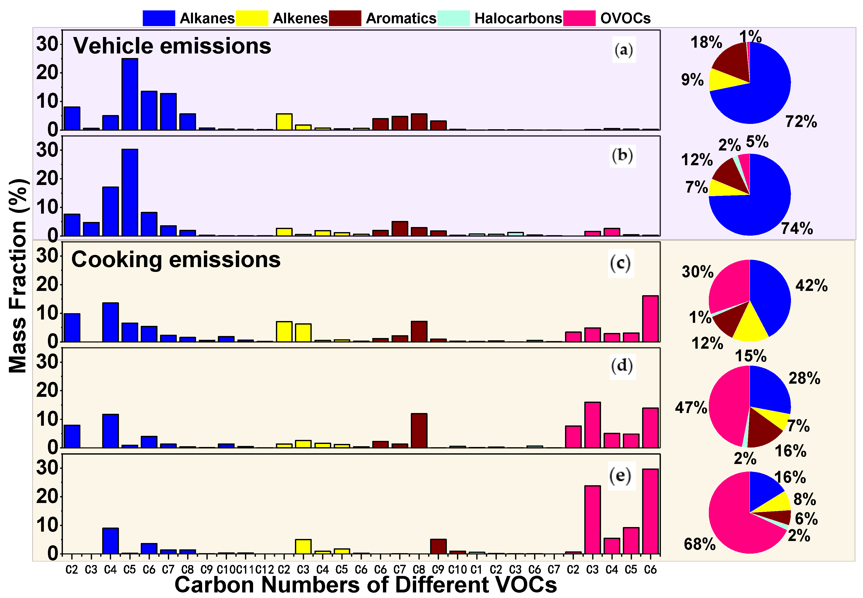
3.1. Emission Characteristics of VOCs from Vehicle and Cooking Emission

The mass fractions of VOCs from vehicle and cooking emissions are shown in Figure 1. All the measured VOCs were categorized into five groups, i.e., alkanes, alkenes, aromatics, halocarbons, and oxygenated carbons (OVOCs). In addition, the five groups are displayed according to their carbon number. When both fuels were used to produce vehicle emissions, alkanes made up the majority of the total VOCs (72% and 74% for pure gasoline and E10, respectively). This result is consistent with Zhang’s roadside measuring study in which the alkane mass fraction was 65% [40]. This percentage increased with the increase in the fraction of ethanol. The peak mass fraction occurred at C5, which was followed by C6 (14%) for gasoline and C4 (17%) for E10, respectively. From the perspective of specific species, isopentane was the most abundant compound when both fuels were used. The fraction of isopentane for using E10 is 24% ± 6%, which is 1.20 times higher than that when gasoline was used (20% ± 3%). Isopentane is the major component in gasoline fuel; so, the dominance of isopentane among the gasoline vehicle exhaust emissions was probably due to the evaporation of gasoline. Previous in situ and laboratory simulation studies also reported that isopentane is dominant among gasoline exhaust emissions [40,41,42]. Besides isopentane, the mass fraction of n-butane for using ethanol fuel was 3.67 times higher than that when gasoline was used. It was reported that ethanol fuel was able to improve the combustion efficiency [43]. This results in a higher proportion of cracking, which may be attributed to the increase in isopentane and n-butane produced by E10. The fractions of alkanes produced by cooking emissions were quite different from those produced by vehicle emissions. The mass fractions were 42%, 28%, and 16% for Bean, Vegetable, and Meat, respectively. This result was within the scope of results from previous in situ measuring results (from 8.51% to 85.07%) [20,44]. Peak mass fractions were found at C4 for all three dishes. Isobutane was the most abundant one. Previous studies reported that isobutane most likely forms due to fuel combustion [45,46]. However, the impact of fuel combustion has been excluded by subtracting blank data. Isobutane was probably producing during the cooking process. Among the three dishes, the cooking of the Meat dish emitted fewer C2 alkanes than the cooking of the Bean and Vegetable dishes did, which may suggest the influence of different ingredients.
The proportion of alkenes emitted by gasoline car fumes (9%) was slightly higher than that emitted by E10 (7%). Ethylene, which is also the product of macromolecular cracking, was the most abundant alkene species, with mass fractions of 6% ± 1%, and 2% ± 3% when gasoline and E10 were used, respectively. The addition of ethanol in gasoline was expected to improve the combustion efficiency because of its higher octane number [47]. For E10, the ethanol content was limited to the extent that macromolecular cracking and the oxidation of ethylene were promoted without continuing the process further. Compared to vehicle emissions, a higher mass fraction of propylene in cooking emissions was the biggest difference. Among the three dishes, Bean had the highest fraction of 6% ± 2%, and Vegetable had the lowest fraction of 3% ± 4%. This discrepancy may be due to the different cooking methods [45].
Aromatics are important components of both vehicle and cooking emissions. In this study, the quantity of aromatics emitted by gasoline cars was 1.5 times higher than that emitted by E10. Previous studies revealed the reduction of aromatics from ethanol fuels [48,49,50]. Aromatics mainly come from the incomplete combustion of fuels [51], which unquestionably suffer a decrease in quantity as the ethanol content increases. Toluene and benzene were the most abundant species in both fuels (Table S6). However, the aromatics produced by cooking emissions showed different characteristics. Vegetable had the largest aromatic fraction of 16%, with the peak mass fraction at C8. Meat had the lowest fraction of 6%, with a peak mass fraction at C9. Aromatics have been reported to be related to cooking ingredients [52]. In this study, we found that cooking vegetable materials emits more aromatics. The Vegetable and Bean dishes emitted more C8 aromatics than the Meat one did, which may be due to the different compositions between plant material (cellulose) and animal material (protein). In terms of individual components, Bean emitted more Toluene (2% ± 1%) and Styrene (2% ± 1%), and Vegetable emitted more styrene (5% ± 2%) and m/p-xylene (4% ± 1%). 1,2,4-Trimethylbenzene (2% ± 1%) and m-ethyltoluene (1% ± 1%) were the most abundant aromatics in Meat. It might be useful to identify the VOCs sources produced by the cooking of different dishes according to the aromatics’ characteristics. One thing to note is that some of the aromatics mentioned above had a relatively low mass fraction. Their concentrations were still above the detection limits, but uncertainties exist. These uncertainties were also due to the differences among the parallel samples, which reflect the instability of aromatics in cooking emissions.
The difference in the VOCs from vehicle emissions between using pure gasoline and E10 are also reflected in the higher fraction of oxygenated VOCs (5%) for E10 fuel, where propanal was the most abundant one, with a mass fraction of 2% ± 2%. Vehicle emissions contain a small quantity of OVOCs. On the contrary, cooking fumes consist of many OVOCs, with mass fractions of 30%, 47%, and 69% for the Bean, Vegetable, and Meat dishes, respectively. The leading role of OVOCs in cooking emissions has also been reported in other literature [19,20]. As shown in Table S6, n-hexanal dominated all three dishes (16%, 14%, and 30%, respectively), besides which, acetone and n-pentanal also simultaneously appeared among the top ten species. Related OVOCs are usually produced by the heating of cooking oil [22]. For example, n-hexanal had been proven to be the breakdown product of linoleic, which is abundant in the corn oil used in this study [53]. The predominance of OVOCs in three dishes may also suggest that cooking oil was likely to determine the VOCs emissions in the cooking process.
There is no doubt that a great discrepancy exists between the two emissions. The alkanes represented by isopentane and OVOCs represented by n-hexanal are endemic species produced by vehicle and cooking emissions, respectively. This may help to identify the two sources.

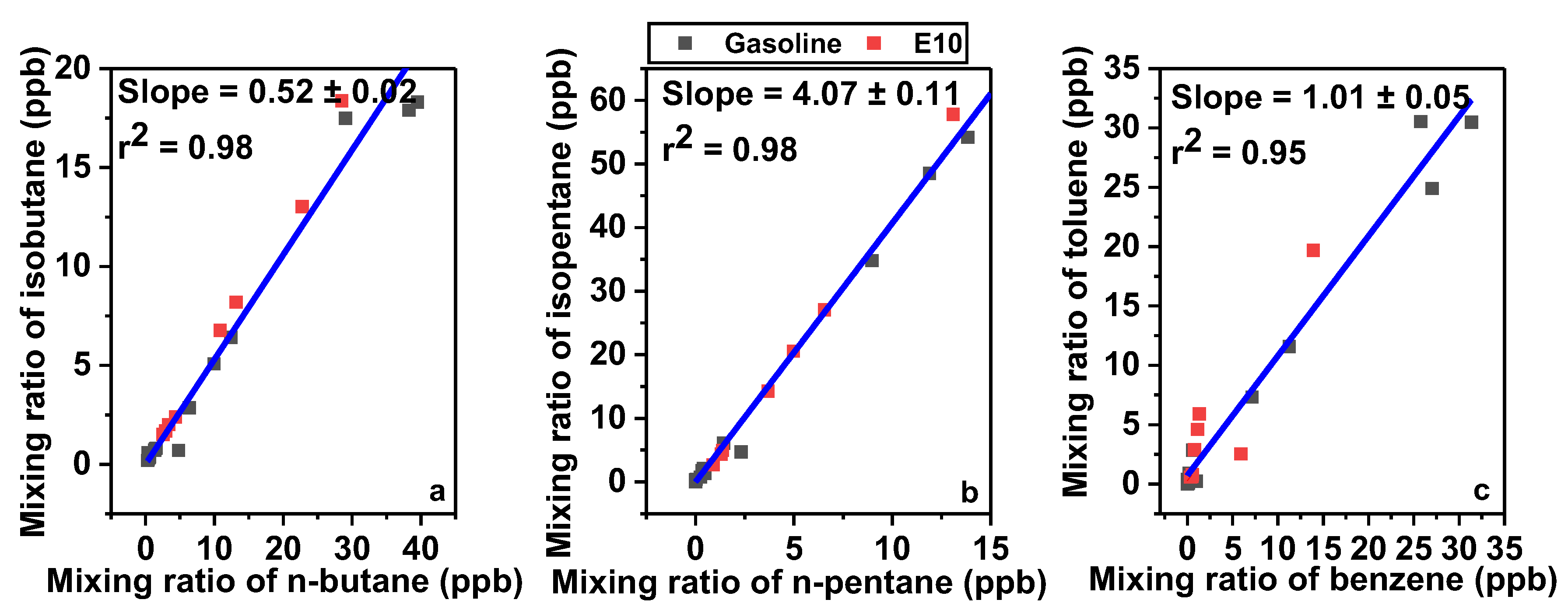
3.2. Characteristic Ratio of VOCs Produced by Vehicle and Cooking Emissions

The ratio of specific VOCs species can be used to identify sources, e.g., isobutane/n-butane, isopentane/n-pentane, and toluene/benzene. Figure 2 shows the ratio of VOCs produced by vehicle emissions (gasoline and E10 as a whole). The ratio of isobutane to n-butane is 0.52 ± 0.02 (Figure 2a), with a good correlation (R2 = 0.98). This result is comparable to that in Huang’s in situ measuring study, which was ~0.58–0.60 [54]. The isopentane/n-pentane ratio in this study is 4.07 ± 0.11 (R2 = 0.98) (Figure 2b), which is similar to the in situ literature value of ~1.82–4.21 [54]. A previous laboratory study demonstrated that the ambient ratio of toluene to benzene (T/B) produced by vehicle exhaust fumes is <2 [55]. Here, we reported a ratio of 1.01 ± 0.05 (R2 = 0.95), which is comparable to that of a previous laboratory study, but lower than that in Huang’s in situ study (3.02–5.15). This discrepancy was likely due to the photochemical process or the influence of other sources near the roadside.
The characteristic VOCs ratios of cooking emissions were investigated in this study. There are plenty of types of cuisines in Chinese cooking; so, it is a great challenge to study the cooking emissions produced by all dishes in detail. Thus, we tried to find commonalities for different cooking VOCs emissions. The correlation coefficients of all VOCs compounds for cooking emission were checked, and the n-hexanal-to-n-pentanal and m/p-xylene-to-o-xylene ratios in all dishes showed the same trend and had a good correlation (Figure 3). The slope of the n-hexanal-to-n-pentanal ratio is 3.68 ± 0.64 (r2 = 0.7880), which is comparable to the results we calculated using Wang and Liang’s data [19,44], whose results were both collected in restaurants. This consistency between our study and previous literature demonstrates that the n-hexanal-to-n-pentanal ratio is a uniquely characteristic ratio for cooking emissions, which is a helpful indicator for differentiating cooking VOCs from ambient air compounds.
The slope of the m/p-xylene-to-o-xylene ratio in this study is 3.91 ± 0.66 (r2 = 0.7964), which is very similar to the result from Liang’s study (slope = 3.32 ± 0.07, r2 = 0.9803), but quite different from Wang’s result (slope = 1.32 ± 0.02, r2 = 0.9937) and that of Cheng’s laboratory study (showed no obvious correlation). This might be due to the different cooking ingredients or cooking styles. Both Wang and Liang’s studies were conducted restaurants, and relative information (e.g., cooking material and the type of oil used) is lacking to perform another analysis. Cheng et al. used a different cooking oil, which might be the reason for the difference.

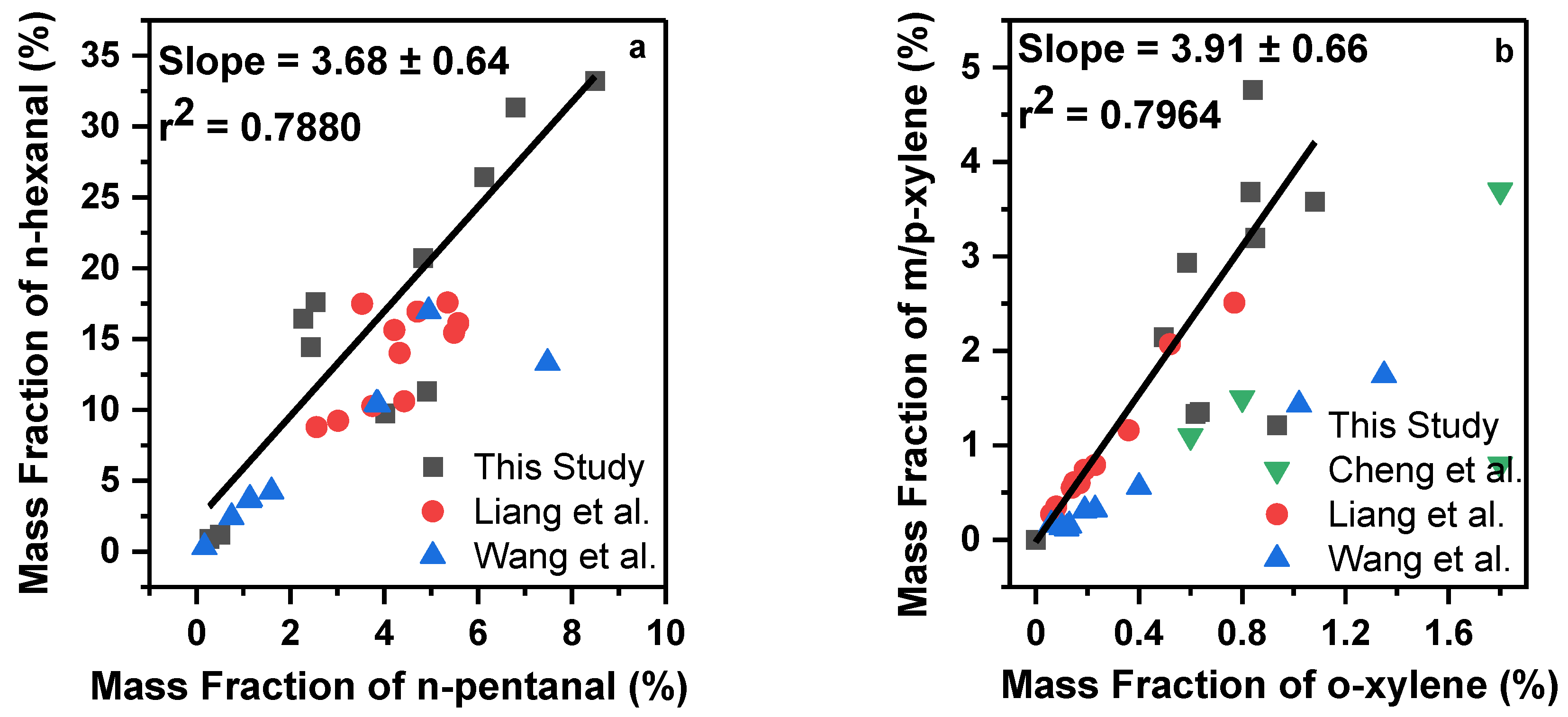
3.3. Comparison of VOCs Produced by Vehicle and Cooking Emissions

In the present work, we used the same dilution system, sampling method, and analysis instrument to measure VOCs produced by vehicle and cooking emissions, which allowed us to conduct a comparison of the VOCs characteristics produced by the two emissions. For vehicle emission, we found similar results as those in previous studies, which are, similar mass fractions of alkanes, the dominance of isopentane, and comparable characteristic ratios. When ethanol was added to the fuel, more butane and fewer aromatics were emitted. Isopentane was dominant in exhaust fumes when both fuels were used. Overall, the VOCs emitted from these two fuels are remarkably similar. This means that E10 has similar VOCs emission characteristics to gasoline and has no advantage if the total emission quantity is ignored.
The VOC emissions produced by cooking fumes are quite different from those produced by vehicle emissions. OVOCs instead of alkanes were the dominant VOCs category. Correspondingly, n-hexanal took the place of isopentane as the most abundant species. Many OVOCs and the leading role of n-hexanal were notable features for cooking emission and are without doubt of importance to differentiate it from other sources.
As for the three dishes, a great discrepancy also exists. For two vegetarian dishes, Bean and Vegetable, had higher alkanes emission characteristics in common, which are significantly different from that of Meat. Additionally, the aromatics emitted by the cooking of the three dishes were diverse from each other. This suggested that for future cooking emission inventories, more detailed classifications are needed, where alkanes and aromatics might be useful indicators to identify different dishes.

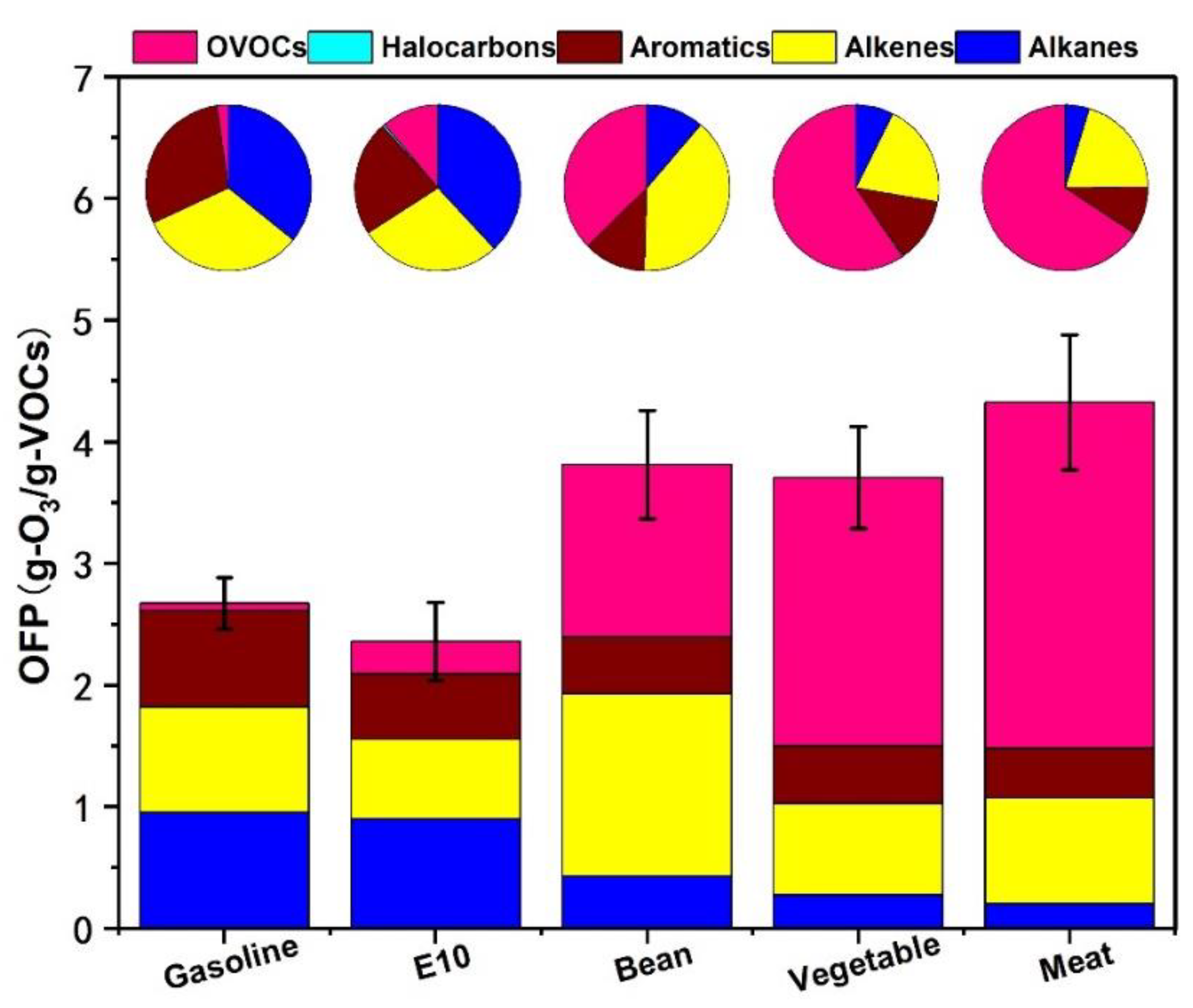
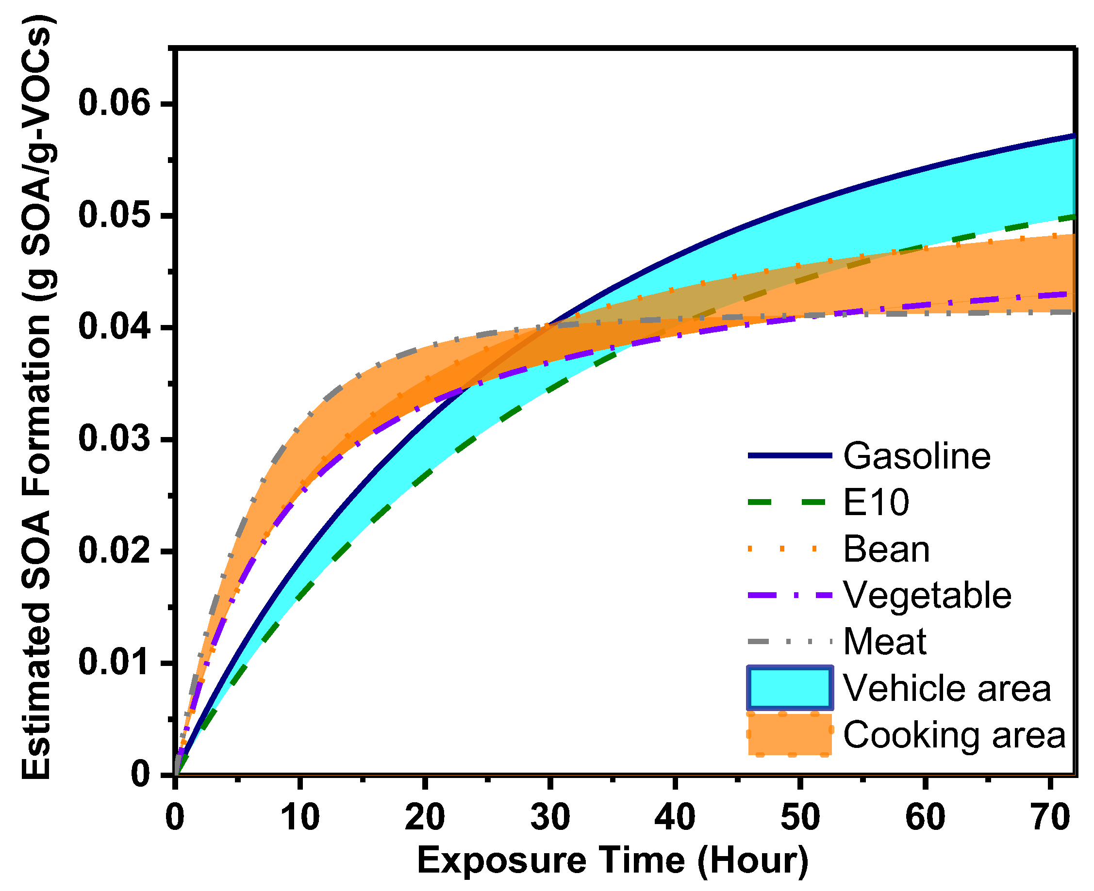
3.4. Ozone and Secondary Organic Aerosol Formation by Vehicle and Cooking Emissions

The ozone formation potential (OFP) of VOCs produced by vehicle and cooking emissions was calculated, where a higher OFP represents a higher capacity of unit mass VOCs to produce more ozone. As shown in Figure 4, alkanes, alkenes, and aromatics dominated the OFP of VOCs produced by vehicle emissions, with a higher OFP having been produced by gasoline (2.67 g O3/g-VOCs) than that of E10 (2.24 g O3/g-VOCs) due to the greater contribution of these three components, as previously demonstrated in other studies [56,57,58]. When considering the top ten species of OFP contribution (Figures S1 and S2), gasoline showed an inclination for alkanes (0.95 g O3/g-VOCs) and aromatics (0.79 g O3/g-VOCs), while OVOCs (0.26 g O3/g-VOCs, mostly propanal and Methyl Vinyl Ketone) were mostly produced by E10. Ethylene, isopentane, toluene, m/p-xylene, and n-pentane are the compounds that significantly contributed to the OFP when both fuels were used.
The OFP of VOCs produced by cooking emissions was consistently higher than that produced by vehicle emissions. Unlike vehicle emission, alkanes and aromatics, such as isopentane, n-pentane, and toluene, key species in vehicle emission, displayed no preponderance for OFP, while OVOCs and alkenes dominated cooking OFP. Among the three dishes, Meat has the highest OFP of 4.62 g O3/g-VOCs, followed by Bean (3.81 g O3/g-VOCs) and Vegetable (3.71 g O3/g-VOCs). From the perspective of the top ten species (Figures S3–S5), n-hexanal, propylene, n-pentanal, and propanal are pivotal compounds in all three dishes. Abundant OVOCs, especially n-hexanal in cooking emissions, might account for its higher OFP than that produced by vehicle emissions.
VOCs were also vital precursors for the formation of secondary organic aerosols. Figure 5 displays the estimated secondary organic aerosol formation of VOCs produced by vehicle and cooking emissions. As shown in Figure 5, a great discrepancy exists between the two emissions. At 72 h of exposure time, gasoline produced the highest SOAF (0.057 ± 0.007 g SOA/g-VOCs), followed by E10 (0.050 ± 0.010 g SOA/g-VOCs), Bean (0.048 ± 0.005 g SOA/g-VOCs), Vegetable (0.043 ± 0.009 g SOA/g-VOCs), and then Meat (0.041 ± 0.001 g SOA/g-VOCs). In general, vehicle emissions can produce more SOAs than cooking emissions can.
From the perspective of specific species, Toluene contributed the most to the total SOAF for vehicle emissions. N-hexanal-derived SOAs dominated the cooking SOAs. Toluene has always been an important precursor for SOA, but the contribution of n-hexanal has never been mentioned before. Our study emphasized the contribution of n-hexanal to form SOAs, and more studies should be conducted in the future.
When comparing the two emissions, the amount of cooking SOAF (orange area in Figure 5) was higher before ~30 h, and that of vehicle SOAF (cyan area) was higher after ~30 h. Thirty hours is the rough time point that was used. What is sure is that, in the first few dozen hours, cooking VOCs produced more SOAs, and in the last few dozen hours, vehicle VOCs produced more SOAs. This could be explained by the dominant OVOCs produced by cooking fumes. Most OVOCs species have higher reaction constants, which allow them to form SOAs faster. This phenomenon may be of great significance in ambient air. When the same masses of cooking fumes and vehicle exhaust fumes are simultaneously emitted into ambient air, cooking fumes can form more SOAs than vehicle emissions can in a short time. However, as time goes by, vehicle exhaust fumes will produce more SOAs in the long term. This result reflects the different time scales at which vehicle and cooking emissions can affect air quality. It should be noted that SOA formation is not only affected by VOCs, but it also determined by other organic precursors, such as intermediate volatile organic compounds (IVOCs) and semi-volatile organic compounds (SVOCs) [59,60,61,62]. Future studies should consider all the potential precursors in SOA formation.

4. Conclusions

Two simulation experiments were conducted to characterize the VOCs emissions produced by vehicle exhaust and cooking fumes. Alkanes and aromatics dominated the VOCs produced by both gasoline and E10, while OVOCs and alkanes were most abundant in cooking fumes. Pentane and n-hexanal were abundant in vehicle and cooking emissions, respectively. This study revealed the differences and similarities of VOCs emitted by vehicle and cooking emissions, which benefits VOC source apportionment studies.
Characteristic ratios of vehicle and cooking emissions were investigated. The isobutane-to-n-butane, isopentane-to-n-pentane, and toluene-to-benzene ratios of vehicle emissions were 0.52 ± 0.02, 4.07 ± 0.11, and 1.01 ± 0.05, respectively, which are also comparable to those in previous studies. The n-hexanal-to-n-pentanal ratio of cooking emissions was 3.68 ± 0.64, which can be treated as an indicator for cooking VOCs. To our knowledge, it is the first time that the characteristic ratio of VOCs produced by cooking fumes has been proposed.
Ozone and secondary organic aerosol formation due to the combustion of vehicle and cooking emissions was estimated. Our results demonstrated that the quantity of OFP was 1.39–1.93 times for cooking emissions than that for vehicle emissions. The quantity of SOAFs produced by vehicle VOCs was 3–38% higher than that produced by cooking VOCs. Controlling cooking emissions can reduce SOA pollution in a short time. However, in the long term, reducing the amount of vehicle emissions is more important for particle pollution. From the current results, the secondary formation contribution of VOCs produced by cooking fumes is comparable to that produced by vehicle exhaust fumes. Our study further emphasizes the importance of cooking emissions. More studies on cooking emissions need to be conducted.
Emission data from two sources in this study enriched the existing results, which can help to establish the VOCs inventories of vehicle and cooking emissions, especially for the latter one. Additionally, the secondary formation estimated in this study highlights the importance of VOCs produced by cooking fumes. More work on cooking emissions is expected in the future.

Supplementary Materials

The following supporting information can be downloaded at: https://www.mdpi.com/article/10.3390/atmos14050806/s1, Table S1: Parameters of the engine used in this study. Table S2: Materials of each dish. Table S3: VOCs species measured in this study. Table S4: MIR values of the VOCs used in this study. Table S5: SOA yield used in this study. Table S6: Top ten species in cooking emissions and vehicle emissions. Figure S1: Top ten species contributing to OFP produced by gasoline emissions. Figure S2: Top ten species contributing to OFP produced by E10 emissions. Figure S3: Top ten species contributing to OFP produced by Bean emissions. Figure S4: Top ten species contributing to OFP produced by Vegetable emissions. Figure S5: Top ten species contributing to OFP produced by Meat emissions.

Author Contributions

Methodology, R.T. (Rui Tan) and S.L. (Sihua Lu); validation, R.T. (Rui Tan), R.T. (Rongzhi Tang), S.L. (Sihua Lu), Y.D. and S.G.; writing—original draft preparation, R.T. (Rui Tan); writing—review and editing, R.T. (Rui Tan), S.L. (Sihua Lu), Y.D. and S.G.; supervision, S.G., D.L. and S.L. (Sihua Lu); funding acquisition, Y.D., S.G.; Experiment design, H.W., W.Z. (Wenfei Zhu), R.T. (Rui Tan), Y.Y., R.S., K.S., W.Z. (Wenbin Zhang), Z.Z., S.L. (Shuangde Li), S.S. and Y.C. All authors have read and agreed to the published version of the manuscript.

Funding

The work was funded by the Open Research Fund of State Environmental Protection Key Laboratory of Vehicle Emission Control and Simulation, Chinese Research Academy of Environmental Sciences (VECS2023S01), the National Natural Science Foundation of China, Creative Research Group Funds (No. 22221004), the National Key Research and Development Program of China (No. 2022YFC3701000, Task 2), and the National Natural Science Foundation of China (No. 41977179, No. 42207118).

Institutional Review Board Statement

Not applicable.

Informed Consent Statement

Informed consent was obtained from all subjects involved in the study.

Data Availability Statement

Data are available upon request from the corresponding author.

Acknowledgments

The authors are sincerely grateful to the support of the Open Research Fund of State Environmental Protection Key Laboratory of Vehicle Emission Control and Simulation, Chinese Research Academy of Environmental Sciences, and the National Natural Science Foundation of China. The authors would also like to thank Yuanju Li for his help with the cooking experiment.

Conflicts of Interest

The authors declare no conflict of interest.

References

  1. Zhu, W.; Zhou, M.; Cheng, Z.; Yan, N.; Huang, C.; Qiao, L.; Wang, H.; Liu, Y.; Lou, S.; Guo, S. Seasonal variation of aerosol compositions in Shanghai, China: Insights from particle aerosol mass spectrometer observations. Sci. Total Environ. 2021, 771, 144948. [Google Scholar] [CrossRef]
  2. Li, J.; Gao, W.; Cao, L.; Xiao, Y.; Zhang, Y.; Zhao, S.; Liu, Z.; Liu, Z.; Tang, G.; Ji, D.; et al. Significant changes in autumn and winter aerosol composition and sources in Beijing from 2012 to 2018: Effects of clean air actions. Environ. Pollut. 2021, 268, 115855. [Google Scholar] [CrossRef]
  3. Guo, S.; Hu, M.; Zamora, M.L.; Peng, J.; Shang, D.; Zheng, J.; Du, Z.; Wu, Z.; Shao, M.; Zeng, L.; et al. Elucidating severe urban haze formation in China. Proc. Natl. Acad. Sci. USA 2014, 111, 17373–17378. [Google Scholar] [CrossRef] [PubMed]
  4. Shen, L.; Wang, Y. Changes in tropospheric ozone levels over the Three Representative Regions of China observed from space by the Tropospheric Emission Spectrometer (TES), 2005–2010. Chin. Sci. Bull. 2012, 57, 2865–2871. [Google Scholar] [CrossRef]
  5. Li, K.; Jacob, D.J.; Liao, H.; Shen, L.; Zhang, Q.; Bates, K.H. Anthropogenic drivers of 2013–2017 trends in summer surface ozone in China. Proc. Natl. Acad. Sci. USA 2019, 116, 422–427. [Google Scholar] [CrossRef]
  6. Guo, S.; Hu, M.; Peng, J.; Wu, Z.; Zamora, M.L.; Shang, D.; Du, Z.; Zheng, J.; Fang, X.; Tang, R.; et al. Remarkable nucleation and growth of ultrafine particles from vehicular exhaust. Proc. Natl. Acad. Sci. USA 2020, 117, 3427–3432. [Google Scholar] [CrossRef] [PubMed]
  7. Wang, H.; Guo, S.; Yu, Y.; Shen, R.; Zhu, W.; Tang, R.; Tan, R.; Liu, K.; Song, K.; Zhang, W.; et al. Secondary aerosol formation from a Chinese gasoline vehicle: Impacts of fuel (E10, gasoline) and driving conditions (idling, cruising). Sci. Total Environ. 2021, 795, 148809. [Google Scholar] [CrossRef] [PubMed]
  8. Wan, Z.; Song, K.; Zhu, W.; Yu, Y.; Wang, H.; Shen, R.; Tan, R.; Lv, D.; Gong, Y.; Yu, X.; et al. A Closure Study of Secondary Organic Aerosol Estimation at an Urban Site of Yangtze River Delta, China. Atmosphere 2022, 13, 1679. [Google Scholar] [CrossRef]
  9. Wang, M.; Li, S.; Zhu, R.; Zhang, R.; Zu, L.; Wang, Y.; Bao, X. On-road tailpipe emission characteristics and ozone formation potentials of VOCs from gasoline, diesel and liquefied petroleum gas fueled vehicles. Atmos. Environ. 2020, 223, 117294. [Google Scholar] [CrossRef]
  10. Hong-Li, W.; Sheng-Ao, J.; Sheng-Rong, L.; Qing-Yao, H.; Li, L.; Shi-Kang, T.; Cheng, H.; Li-Ping, Q.; Chang-Hong, C. Volatile organic compounds (VOCs) source profiles of on-road vehicle emissions in China. Sci. Total Environ. 2017, 607–608, 253–261. [Google Scholar] [CrossRef]
  11. Lv, D.; Lu, S.; Tan, X.; Shao, M.; Xie, S.; Wang, L. Source profiles, emission factors and associated contributions to secondary pollution of volatile organic compounds (VOCs) emitted from a local petroleum refinery in Shandong. Environ. Pollut. 2021, 274, 116589. [Google Scholar] [CrossRef]
  12. Mo, Z.; Shao, M.; Lu, S.; Qu, H.; Zhou, M.; Sun, J.; Gou, B. Process-specific emission characteristics of volatile organic compounds (VOCs) from petrochemical facilities in the Yangtze River Delta, China. Sci. Total Environ. 2015, 533, 422–431. [Google Scholar] [CrossRef] [PubMed]
  13. Lv, D.; Lu, S.; He, S.; Song, K.; Shao, M.; Xie, S.; Gong, Y. Research on accounting and detection of volatile organic compounds from a typical petroleum refinery in Hebei, North China. Chemosphere 2021, 281, 130653. [Google Scholar] [CrossRef]
  14. Qin, J.; Wang, X.; Yang, Y.; Qin, Y.; Shi, S.; Xu, P.; Chen, R.; Zhou, X.; Tan, J.; Wang, X. Source apportionment of VOCs in a typical medium-sized city in North China Plain and implications on control policy. J. Environ. Sci. 2021, 107, 26–37. [Google Scholar] [CrossRef]
  15. Wang, D.; Zhou, J.; Han, L.; Tian, W.; Wang, C.; Li, Y.; Chen, J. Source apportionment of VOCs and ozone formation potential and transport in Chengdu, China. Atmos. Pollut. Res. 2023, 14, 101730. [Google Scholar] [CrossRef]
  16. Wu, Y.; Fan, X.; Liu, Y.; Zhang, J.; Wang, H.; Sun, L.; Fang, T.; Mao, H.; Hu, J.; Wu, L.; et al. Source apportionment of VOCs based on photochemical loss in summer at a suburban site in Beijing. Atmos. Environ. 2023, 293, 119459. [Google Scholar] [CrossRef]
  17. Wang, B.; Liu, Z.; Li, Z.; Sun, Y.; Wang, C.; Zhu, C.; Sun, L.; Yang, N.; Bai, G.; Fan, G.; et al. Characteristics, chemical transformation and source apportionment of volatile organic compounds (VOCs) during wintertime at a suburban site in a provincial capital city, east China. Atmos. Environ. 2023, 298, 119621. [Google Scholar] [CrossRef]
  18. Han, Y.; Wang, T.; Li, R.; Fu, H.; Duan, Y.; Gao, S.; Zhang, L.; Chen, J. Measurement report: Volatile organic compound characteristics of the different land-use types in Shanghai: Spatiotemporal variation, source apportionment and impact on secondary formations of ozone and aerosol. Atmos. Chem. Phys. 2023, 23, 2877–2900. [Google Scholar] [CrossRef]
  19. Wang, H.; Xiang, Z.; Wang, L.; Jing, S.; Lou, S.; Tao, S.; Liu, J.; Yu, M.; Li, L.; Lin, L.; et al. Emissions of volatile organic compounds (VOCs) from cooking and their speciation: A case study for Shanghai with implications for China. Sci. Total Environ. 2018, 621, 1300–1309. [Google Scholar] [CrossRef]
  20. He, W.-Q.; Shi, A.-J.; Shao, X.; Nie, L.; Wang, T.-Y.; Li, G.-H. Insights into the comprehensive characteristics of volatile organic compounds from multiple cooking emissions and aftertreatment control technologies application. Atmos. Environ. 2020, 240, 117646. [Google Scholar] [CrossRef]
  21. Yi, H.; Huang, Y.; Tang, X.; Zhao, S.; Xie, X.; Zhang, Y. Characteristics of non-methane hydrocarbons and benzene series emission from commonly cooking oil fumes. Atmos. Environ. 2019, 200, 208–220. [Google Scholar] [CrossRef]
  22. Zhang, D.-C.; Liu, J.-J.; Jia, L.-Z.; Wang, P.; Han, X. Speciation of VOCs in the cooking fumes from five edible oils and their corresponding health risk assessments. Atmos. Environ. 2019, 211, 6–17. [Google Scholar] [CrossRef]
  23. Ari, A.; Arı, P.E.; Yenisoy-Karakaş, S.; Gaga, E.O. Source characterization and risk assessment of occupational exposure to volatile organic compounds (VOCs) in a barbecue restaurant. Build. Environ. 2020, 174, 106791. [Google Scholar] [CrossRef]
  24. Huang, X.; Han, D.; Cheng, J.; Chen, X.; Zhou, Y.; Liao, H.; Dong, W.; Yuan, C. Characteristics and health risk assessment of volatile organic compounds (VOCs) in restaurants in Shanghai. Environ. Sci. Pollut. Res. 2020, 27, 490–499. [Google Scholar] [CrossRef]
  25. Lu, F.; Shen, B.; Li, S.; Liu, L.; Zhao, P.; Si, M. Exposure characteristics and risk assessment of VOCs from Chinese residential cooking. J. Environ. Manag. 2021, 289, 112535. [Google Scholar] [CrossRef]
  26. Zhang, Z.; Zhu, W.; Hu, M.; Wang, H.; Chen, Z.; Shen, R.; Yu, Y.; Tan, R.; Guo, S. Secondary Organic Aerosol from Typical Chinese Domestic Cooking Emissions. Environ. Sci. Technol. Lett. 2021, 8, 24–31. [Google Scholar] [CrossRef]
  27. Zhang, Z.; Zhu, W.; Hu, M.; Liu, K.; Wang, H.; Tang, R.; Shen, R.; Yu, Y.; Tan, R.; Song, K.; et al. Formation and evolution of secondary organic aerosols derived from urban-lifestyle sources: Vehicle exhaust and cooking emissions. Atmos. Chem. Phys. 2021, 21, 15221–15237. [Google Scholar] [CrossRef]
  28. Zhu, W.; Guo, S.; Zhang, Z.; Wang, H.; Yu, Y.; Chen, Z.; Shen, R.; Tan, R.; Song, K.; Liu, K.; et al. Mass spectral characterization of secondary organic aerosol from urban cooking and vehicular sources. Atmos. Chem. Phys. 2021, 21, 15065–15079. [Google Scholar] [CrossRef]
  29. Carter, W.P. Development of the SAPRC-07 chemical mechanism. Atmos. Environ. 2010, 44, 5324–5335. [Google Scholar] [CrossRef]
  30. Yuan, B.; Hu, W.; Shao, M.; Wang, M.; Chen, W.; Lu, S.; Zeng, L.; Hu, M. VOC emissions, evolutions and contributions to SOA formation at a receptor site in eastern China. Atmos. Chem. Phys. 2013, 13, 8815–8832. [Google Scholar] [CrossRef]
  31. Yu, Y.; Wang, H.; Wang, T.; Song, K.; Tan, T.; Wan, Z.; Gao, Y.; Dong, H.; Chen, S.; Zeng, L.; et al. Elucidating the importance of semi-volatile organic compounds to secondary organic aerosol formation at a regional site during the EXPLORE-YRD campaign. Atmos. Environ. 2021, 246, 118043. [Google Scholar] [CrossRef]
  32. Lim, Y.B.; Ziemann, P.J. Effects of Molecular Structure on Aerosol Yields from OH Radical-Initiated Reactions of Linear, Branched, and Cyclic Alkanes in the Presence of NOx. Environ. Sci. Technol. 2009, 43, 2328–2334. [Google Scholar] [CrossRef]
  33. Chan, A.W.H.; Kautzman, K.; Chhabra, P.; Surratt, J.; Chan, M.; Crounse, J.; Kurten, A.; Wennberg, P.; Flagan, R.; Seinfeld, J. Secondary organic aerosol formation from photooxidation of naphthalene and alkylnaphthalenes: Implications for oxidation of intermediate volatility organic compounds (IVOCs). Atmos. Chem. Phys. 2009, 9, 3049–3060. [Google Scholar] [CrossRef]
  34. Ng, N.; Kroll, J.; Chan, A.; Chhabra, P.; Flagan, R.; Seinfeld, J. Secondary organic aerosol formation from m-xylene, toluene, and benzene. Atmos. Chem. Phys. 2007, 7, 3909–3922. [Google Scholar] [CrossRef]
  35. Zhang, X.; Cappa, C.; Jathar, S.; McVay, R.; Ensberg, J.; Kleeman, M.; Seinfeld, J. Influence of vapor wall loss in laboratory chambers on yields of secondary organic aerosol. Proc. Natl. Acad. Sci. USA 2014, 111, 5802–5807. [Google Scholar] [CrossRef]
  36. Gao, Y.; Wang, H.; Zhang, X.; Jing, S.; Peng, Y.; Qiao, L.; Zhou, M.; Huang, D.; Wang, Q.; Li, X.; et al. Estimating Secondary Organic Aerosol Production from Toluene Photochemistry in a Megacity of China. Environ. Sci. Technol. 2019, 53, 8664–8671. [Google Scholar] [CrossRef]
  37. Wang, H.; Wang, Q.; Gao, Y.; Zhou, M.; Jing, S.; Qiao, L.; Yuan, B.; Huang, D.; Huang, C.; Lou, S.; et al. Estimation of Secondary Organic Aerosol Formation During a Photochemical Smog Episode in Shanghai, China. J. Geophys. Res. Atmos. 2020, 125, e2019JD032033. [Google Scholar] [CrossRef]
  38. Zhang, H.; Chen, C.; Yan, W.; Wu, N.; Bo, Y.; Zhang, Q.; He, K. Characteristics and sources of non-methane VOCs and their roles in SOA formation during autumn in a central Chinese city. Sci. Total Environ. 2021, 782, 146802. [Google Scholar] [CrossRef] [PubMed]
  39. Grosjean, D.; Seinfeld, J.H. Parameterization of the formation potential of secondary organic aerosols. Atmos. Environ. (1967) 1989, 23, 1733–1747. [Google Scholar] [CrossRef]
  40. Zhang, Q.; Sun, L.; Wei, N.; Wu, L.; Mao, H. The characteristics and source analysis of VOCs emissions at roadside: Assess the impact of ethanol-gasoline implementation. Atmos. Environ. 2021, 263, 118670. [Google Scholar] [CrossRef]
  41. Song, C.; Liu, Y.; Sun, L.; Zhang, Q.; Mao, H. Emissions of volatile organic compounds (VOCs) from gasoline- and liquified natural gas (LNG)-fueled vehicles in tunnel studies. Atmos. Environ. 2020, 234, 117626. [Google Scholar] [CrossRef]
  42. Cao, X.; Yao, Z.; Shen, X.; Ye, Y.; Jiang, X. On-road emission characteristics of VOCs from light-duty gasoline vehicles in Beijing, China. Atmos. Environ. 2016, 124, 146–155. [Google Scholar] [CrossRef]
  43. Thakur, A.K.; Kaviti, A.K. Progress in regulated emissions of ethanol-gasoline blends from a spark ignition engine. Biofuels 2021, 12, 197–220. [Google Scholar] [CrossRef]
  44. Liang, X.; Chen, L.; Liu, M.; Lu, Q.; Lu, H.; Gao, B.; Zhao, W.; Sun, X.; Xu, J.; Ye, D. Carbonyls from commercial, canteen and residential cooking activities as crucial components of VOC emissions in China. Sci. Total Environ. 2022, 846, 157317. [Google Scholar] [CrossRef]
  45. Cheng, S.; Wang, G.; Lang, J.; Wen, W.; Wang, X.; Yao, S. Characterization of volatile organic compounds from different cooking emissions. Atmos. Environ. 2016, 145, 299–307. [Google Scholar] [CrossRef]
  46. Mugica, V.; Vega, E.; Chow, J.; Reyes, E.; Sanchez, G.; Arriaga, J.; Egami, R.; Watson, J. Speciated non-methane organic compounds emissions from food cooking in Mexico. Atmos. Environ. 2001, 35, 1729–1734. [Google Scholar] [CrossRef]
  47. Yoon, S.H.; Ha, S.; Roh, H.; Lee, C. Effect of bioethanol as an alternative fuel on the emissions reduction characteristics and combustion stability in a spark ignition engine. Proc. Inst. Mech. Eng. Part D J. Automob. Eng. 2009, 223, 941–951. [Google Scholar] [CrossRef]
  48. Yao, Y.-C.; Tsai, J.-H.; Wang, I.; Tsai, H.-R. Investigating Criteria and Organic Air pollutant Emissions from Motorcycles by Using Various Ethanol-Gasoline Blends. Aerosol Air Qual. Res. 2017, 17, 167–175. [Google Scholar] [CrossRef]
  49. Lin, Y.-C.; Jhang, S.-R.; Lin, S.-L.; Chen, K.-S. Comparative effect of fuel ethanol content on regulated and unregulated emissions from old model vehicles: An assessment and policy implications. Atmos. Pollut. Res. 2021, 12, 66–75. [Google Scholar] [CrossRef]
  50. Li, L.; Ge, Y.; Wang, M.; Peng, Z.; Song, Y.; Zhang, L.; Yuan, W. Exhaust and evaporative emissions from motorcycles fueled with ethanol gasoline blends. Sci. Total Environ. 2015, 502, 627–631. [Google Scholar] [CrossRef]
  51. Liang, X.J.; Li, X.Q. Research on Emissions of Benzene & Polycyclic Aromatic Hydrocarbons in Constant Volume Combustion Bomb. Adv. Mater. Res. 2012, 468–471, 2993–2997. [Google Scholar]
  52. Atamaleki, A.; Zarandi, S.M.; Massoudinejad, M.; Esrafili, A.; Khaneghah, A.M. Emission of BTEX compounds from the frying process: Quantification, environmental effects, and probabilistic health risk assessment. Environ. Res. 2022, 204, 112295. [Google Scholar] [CrossRef]
  53. Goicoechea, E.; Guillén, M.D. Volatile compounds generated in corn oil stored at room temperature. Presence of toxic compounds. Eur. J. Lipid Sci. Technol. 2014, 116, 395–406. [Google Scholar] [CrossRef]
  54. Huang, Y.; Ling, Z.; Lee, S.; Ho, S.; Cao, J.; Blake, D.; Cheng, Y.; Lai, S.; Ho, K.; Gao, Y.; et al. Characterization of volatile organic compounds at a roadside environment in Hong Kong: An investigation of influences after air pollution control strategies. Atmos. Environ. 2015, 122, 809–818. [Google Scholar] [CrossRef]
  55. Yang, W.; Zhang, Q.; Wang, J.; Zhou, C.; Zhang, Y.; Pan, Z. Emission characteristics and ozone formation potentials of VOCs from gasoline passenger cars at different driving modes. Atmos. Pollut. Res. 2018, 9, 804–813. [Google Scholar] [CrossRef]
  56. Tibaquirá, J.E.; Huertas, J.; Ospina, S.; Quirama, L.; Niño, J. The Effect of Using Ethanol-Gasoline Blends on the Mechanical, Energy and Environmental Performance of In-Use Vehicles. Energies 2018, 11, 221. [Google Scholar] [CrossRef]
  57. Yao, Y.-C.; Tsai, J.-H.; Chou, H.-H. Air Pollutant Emission Abatement using Application of Various Ethanol-gasoline Blends in High-mileage Vehicles. Aerosol Air Qual. Res. 2011, 11, 547–559. [Google Scholar] [CrossRef]
  58. Zhang, M.; Ge, Y.; Wang, X.; Thomas, D.; Su, S.; Li, H. An assessment of how bio-E10 will impact the vehicle-related ozone contamination in China. Energy Rep. 2020, 6, 572–581. [Google Scholar] [CrossRef]
  59. Tang, R.; Lu, Q.; Guo, S.; Wang, H.; Song, K.; Yu, Y.; Tan, R.; Liu, K.; Shen, R.; Chen, S.; et al. Measurement report: Distinct emissions and volatility distribution of intermediate-volatility organic compounds from on-road Chinese gasoline vehicles: Implication of high secondary organic aerosol formation potential. Atmos. Chem. Phys. 2021, 21, 2569–2583. [Google Scholar] [CrossRef]
  60. Yu, Y.; Guo, S.; Wang, H.; Shen, R.; Zhu, W.; Tan, R.; Song, K.; Zhang, Z.; Li, S.; Chen, Y.; et al. Importance of Semivolatile/Intermediate-Volatility Organic Compounds to Secondary Organic Aerosol Formation from Chinese Domestic Cooking Emissions. Environ. Sci. Technol. Lett. 2022, 9, 507–512. [Google Scholar] [CrossRef]
  61. Zhang, Y.; Fan, J.; Song, K.; Gong, Y.; Lv, D.; Wan, Z.; Li, T.; Zhang, C.; Lu, S.; Chen, S.; et al. Secondary Organic Aerosol Formation from Semi-Volatile and Intermediate Volatility Organic Compounds in the Fall in Beijing. Atmosphere 2023, 14, 94. [Google Scholar] [CrossRef]
  62. Song, K.; Guo, S.; Gong, Y.; Lv, D.; Wan, Z.; Zhang, Y.; Fu, Z.; Hu, K.; Lu, S. Non-target scanning of organics from cooking emissions using comprehensive two-dimensional gas chromatography-mass spectrometer (GC×GC-MS). Appl. Geochem. 2023, 151, 105601. [Google Scholar] [CrossRef]
Figure 1. Emission characteristics of VOCs from vehicle exhaust and cooking fumes. (a) Gasoline; (b) E10; (c) Bean; (d) Vegetable; (e) Meat. Blue stands for alkanes, yellow stands for alkenes, red stands for aromatics, cyan stands for halocarbons, and pink stands for OVOCs.
Atmosphere 14 00806 g001
Figure 2. Characteristic ratio from vehicle emission; pink dots stand for gasoline data; black dots stand for data from using E10. The blue line is the fitting curve of all the data used. (a) The ratio of isobutane to n-butane. (b) the ratio of isopentane to n-pentane; (c) the ratio of toluene to benzene.
Atmosphere 14 00806 g002
Figure 3. Comparison of characteristic ratios from cooking emission. Black squares stand for the data in this study; pink circles stand for data from Liang’s study; blue triangles stand for data from Wang’s study; green triangles stand for data from Cheng’s study. The black line is the fitting curve using data from this study. (a) The ratio of n-hexanal to n-pentanal. (b) the ratio of m/p-xylene to o-xylene [19,44,45].
Atmosphere 14 00806 g003
Figure 4. Ozone formation potential of VOCs from vehicle and cooking emissions. Columns represent the ozone formation for the unit mass of VOCs from different sources, and pie charts represent the relative contribution (%) of different VOCs categories. Pink represents OVOCs; cyan represents halocarbons; red represents aromatics; yellow represents alkenes; blue represents alkanes.
Atmosphere 14 00806 g004
Figure 5. Estimated SOA formation of VOCs produced by vehicle and cooking emissions; cyan area represents the SOAF for vehicle-emitted VOCs; orange area represents the SOAF for cooking-emitted VOCs.
Atmosphere 14 00806 g005
Disclaimer/Publisher’s Note: The statements, opinions and data contained in all publications are solely those of the individual author(s) and contributor(s) and not of MDPI and/or the editor(s). MDPI and/or the editor(s) disclaim responsibility for any injury to people or property resulting from any ideas, methods, instructions or products referred to in the content.

