Precipitation Nowcasting Based on Deep Learning over Guizhou, China

Abstract

Accurate precipitation nowcasting (lead time: 0–2 h), which requires high spatiotemporal resolution data, is of great relevance in many weather-dependent social and operational activities. In this study, we are aiming to construct highly accurate deep learning (DL) models to directly obtain precipitation nowcasting at 6-min intervals for the lead time of 0–2 h. The Convolutional Long Short-Term Memory (ConvLSTM) and Predictive Recurrent Neural Network (PredRNN) models were used as comparative DL models, and the Lucas–Kanade (LK) Optical Flow method was selected as a traditional extrapolation baseline. The models were trained with high-quality datasets (resolution: 1 min) created from precipitation observations recorded by automatic weather stations in Guizhou Province (China). A comprehensive evaluation of the precipitation nowcasting was performed, which included consideration of the root mean square error, equitable threat score (ETS), and probability of detection (POD). The evaluation indicated that the reduction of the number of missing values and data normalization boosted training efficiency and improved the forecasting skill of the DL models. Increasing the time series length of the training set and the number of training samples both improved the POD and ETS of the DL models and enhanced nowcasting stability with time. Training with the Hea-P dataset further improved the forecasting skill of the DL models and sharply increased the ETS for thresholds of 2.5, 8, and 15 mm, especially for the 1-h lead time. The PredRNN model trained with the Hea-P dataset (time series length: 8 years) outperformed the traditional LK Optical Flow method for all thresholds (0.1, 1, 2.5, 8, and 15 mm) and obtained the best performance of all the models considered in this study in terms of ETS. Moreover, the Method for Object-Based Diagnostic Evaluation on a rainstorm case revealed that the PredRNN model, trained well with high-quality observation data, could both capture complex nonlinear characteristics of precipitation more accurately than achievable using the LK Optical Flow method and establish a reasonable mapping network during drastic changes in precipitation. Thus, its results more closely matched the observations, and its forecasting skill for thresholds exceeding 8 mm was improved substantially.

1. Introduction

Precipitation nowcasting means forecasting precipitation with a lead time of 0–2 h, focusing more on mesoscale–microscale weather systems at a high spatiotemporal resolution [1,2,3]. Highly accurate precipitation nowcasting is vital in support of various operational activities, e.g., disaster relief, energy management, and flood early warning systems. Consequently, the accuracy of precipitation nowcasting has a critical socioeconomic impact.

Currently, the primary means of improving the accuracy of precipitation nowcasting involve the integration of extrapolation and ensemble numerical weather prediction (NWP) [4,5,6,7,8]. However, literature shows that global coarse-resolution NWP models have challenges in generating accurate precipitation with a lead time of 0–2 h [9,10], affected by the spin-up issue and the difficulties in non-Gaussian data assimilation. Although convection-permitting models with high resolution could greatly improve performance, these models are computationally expensive. Traditional integration of extrapolation methods, such as cross-correlation tracking and optical flow, has been used widely in operational weather forecasting [11,12,13,14,15,16,17,18,19]. Still, they exhibit a marked reduction in forecasting skills with increasing lead time owing to their linear operating limits and their deficiencies in forecasting storm growth and decay [20].

In recent years, the application of deep learning (DL) [21] has become popular in the field of meteorology [22,23,24] owing to its nonlinear operation, and it has achieved substantial advances in terms of quantitative precipitation nowcasting using radar echo extrapolation [25,26,27,28,29,30,31,32]. In comparison with the traditional integration of extrapolation and NWP, DL models can realize relatively accurate precipitation nowcasting. For example, Shi et al. [27] involved the convolution operation in input-to-state and state-to-state transitions in the transformation of a two-dimensional image into a three-dimensional tensor and proposed the Convolutional Long Short-Term Memory (ConvLSTM) model. This approach, which was shown capable of effectively capturing spatial correlations and further realizing the extrapolation of spatiotemporal sequences, was applied to achieve quantitative precipitation nowcasting. Subsequently, they involved the convolution operation in the recurrent gated unit (GRU) and used a subnetwork to output a location-variant connection structure before performing state transitions. Then, they proposed the trajectory GRU that could handle the spatial correlations better and perform more accurately than previous methods [28]. Wang et al. [29] designed the Spatiotemporal LSTM (ST-LSTM) model that can transfer memories vertically and horizontally, and then they proposed the Predictive Recurrent Neural Network (PredRNN) model. To strengthen the power for modeling short-term dynamics and to alleviate the vanishing gradient problem, they improved the PredRNN model to PredRNN++ [30], which incorporates a cascaded dual-memory structure and a gradient highway unit. Ji et al. [31] exploited the advantages of different DL model architectures in combination with the ConvLSTM unit in the U-Net generator and proposed the CLGAN model, which can better capture the precipitation object and its characteristics. Chen et al. [32] compared and analyzed the extrapolation prediction of radar echoes using the ConvGRU method, cross-correlation method, optical flow method, and particle filter method and found that the output of the ConvGRU method more closely matched the location, intensity, and shape of actual radar echoes. Many other studies have modified existing techniques to obtain relatively better nowcasting performance in comparison with that achieved using the integration of extrapolation [33,34,35,36,37,38,39,40,41,42,43,44,45,46,47]. However, precipitation calculated from radar echoes is based on the Z–R relationship. We believe that the Z–R relationship cannot describe the nonlinear relationship between a radar echo and precipitation. Moreover, it is difficult to avoid calculation errors derived from the Z–R relationship. Factors such as radar model, detection range, and clutter interference will lead to poor universality of a DL model. Consequently, the objective of this study was to construct DL models for precipitation nowcasting based on precipitation observation data, which could directly obtain precipitation nowcasting.

The reason we use DL models is their nonlinear operation, and the ConvLSTM model is one of the classical models used in the precipitation nowcasting problem. It can extract the spatial characteristics while capturing the time characteristics efficiently. PredRNN improved memory information by transferring memories vertically and horizontally, and it can perform better for forecast time compared with ConvLSTM. The Lucas–Kanade Optical Flow (LK Optical Flow) is a good method that improved optical flow vector calculation for traditional optical flow [48], and it was selected as a traditional baseline. We hope to compare the two typical DL models with LK Optical Flow and try to construct highly accurate models based on precipitation observation data.

In this study, we formed two high-quality datasets: a pre-processed precipitation dataset (Pre-P dataset) and a heavy precipitation dataset (Hea-P dataset). Then, we constructed precipitation DL models that could directly obtain precipitation nowcasting based on precipitation observation data. Furthermore, we improved the forecasting skill of the DL models by increasing the length of the time series of the training set and by training with the Hea-P dataset. The study area selected was Guizhou Province in China (29.2–24.7° N, 103.6–109.6° E), which features highly complex terrain and frequently experiences geological disasters and floods [49,50]. Moreover, the region is also lacking in terms of high-accuracy precipitation nowcasting.

The remainder of this manuscript is organized as follows. Section 2 describes the data and methods used in the study. Section 3 comprehensively evaluates both the DL models trained with different datasets and the LK Optical Flow method. Finally, the conclusions and a discussion are presented in Section 4.

2. Data and Method

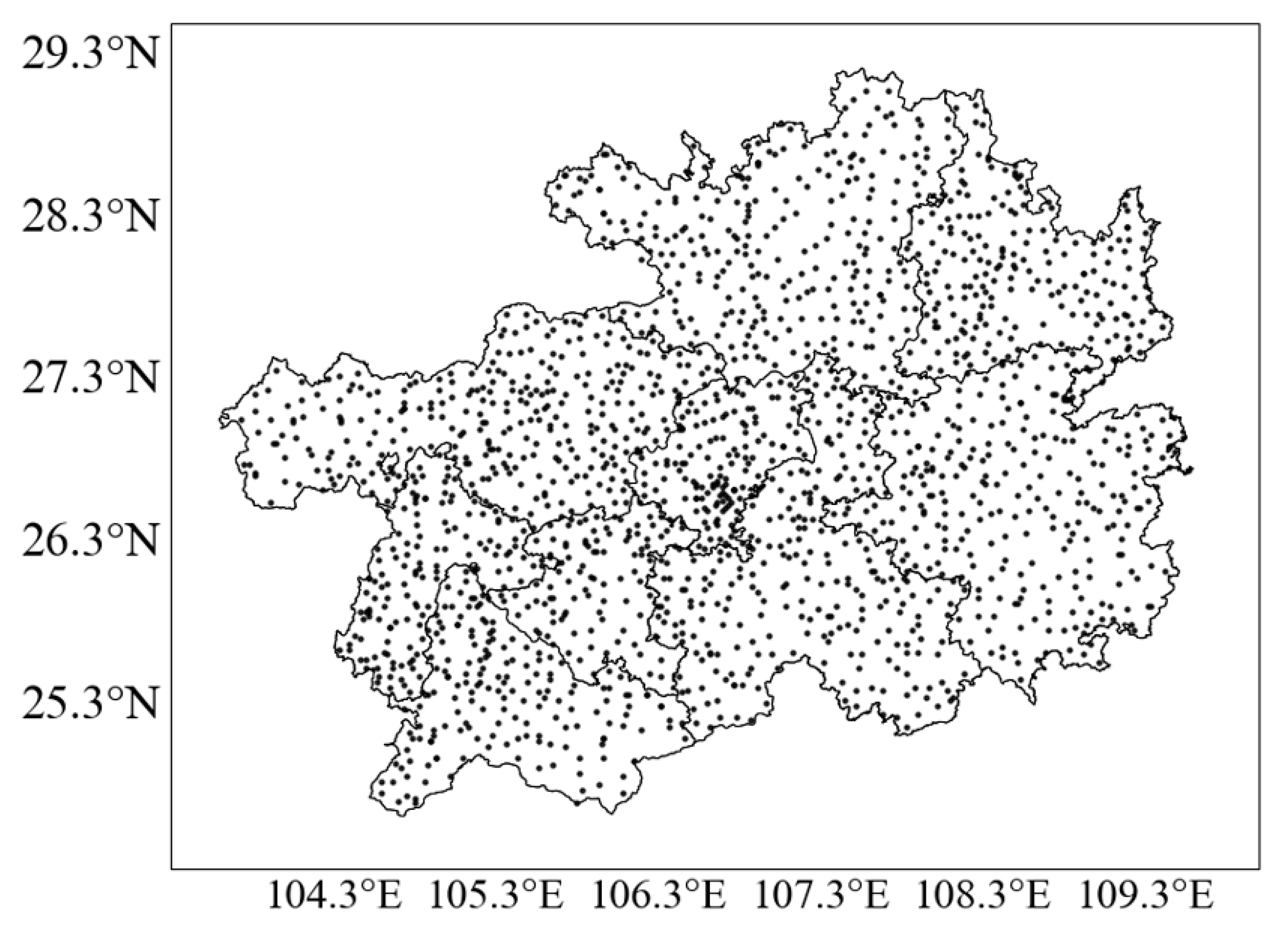
2.1. Guizhou Automatic Weather Station (AWS) Observations

High-quality real-time precipitation observation data (resolution: 1 min) recorded over a nine-year period from 20:00 (all times UTC+8) on 31 December 2012 to 20:00 on 31 December 2021 (observation day: from 20:00 on the previous day to 20:00 on the same day) by 1835 automatic weather stations (AWS) in Guizhou Province (as shown in Figure 1) were obtained from the Guizhou Meteorological Information Center.

2.2. Pre-Processed Precipitation Dataset (Pre-P Dataset)

The number of missing values in the observation data was reduced using the neighborhood method (where the time series before and after the missing values and the data of nearby stations were complete). Then, the bilinear interpolation method was used to interpolate station data within the region 24.5–29.5° N, 103.5–110° E to the gridded field (resolution: 0.125° × 0.125°). Data normalization resulted in a high-quality dataset with a range of variation of [0, 1]. Ultimately, the pre-processed(Pre-P) dataset was formed, comprising 788,400 samples.

2.3. Heavy Precipitation Dataset (Hea-P Dataset)

Data in the Pre-P dataset from May–September in each of the nine years from 2013–2021 were selected, and samples with little or no precipitation were removed. Consequently, the heavy precipitation (Hea-P) dataset was determined, comprising 332,640 samples.

2.4. Lucas–Kanade (LK) Optical Flow Method

The optical flow method is defined as a method for calculating the intensity of image pixel points over time to infer the speed and direction of object movement. It finds the correspondence between the previous and the current frame based on changes in the pixels of the image in the time series and the correlation between adjacent frames, from which it calculates the motion information of objects between adjacent frames. This study employed the LK Optical Flow method [48], the process of which can be divided into two steps:

In the first step, the optical flow vector field is calculated. The instantaneous velocity two-dimensional vector field of the changing trend of grayscale at each point on the image and the optical flow vector field are solved using the following three basic assumptions.

(1) The brightness is constant, i.e., when the same target moves between different frames, the brightness will not change in any way. According to this assumption, the basic equation of the optical flow method can be obtained:

$$I\left(x,y,t\right)=I\left(x+dx,y+dy,t+dt\right)$$

(1)

where x and y are the coordinate positions of a pixel in the image, t is the time series in which the image is located, and (dx, dy) is the distance moved to the next frame, using dt time, i.e., the light intensity of the pixel before and after motion has remained constant.

(2) The movement in continuous time is a ‘small movement’, which means that the change of time will not cause a drastic change in the target position. Expanding the Taylor section of Equation (1) yields:

$$\left(x,y,t\right)=I\left(x,y,t+\frac{\partial I}{\partial x}dx+\frac{\partial I}{\partial y}dy+\frac{\partial I}{\partial t}dt+\epsilon \right),$$

(2)

where ε represents a second-order infinitesimal term that is negligible. Assuming the velocity vectors u and v of the optical flow in the x-axis and y-axis directions, the formulas will be as follows:

$$Iu=\frac{dx}{dt}, v=\frac{dy}{dt},$$

(3)

The partial derivatives of the gray scale of pixel points in the image on x, y, and t are as follows:

$$I_x=\frac{\partial I}{\partial x}, I_y=\frac{\partial I}{\partial y}, I_t=\frac{\partial I}{\partial t},$$

(4)

Then, substituting Equation (2) into Equation (1) and dividing by dt gives the following:

$$I_{x}u+I_{y}v+I_t=0,$$

(5)

where I_x, I_y, and I_z can be obtained from image data, and (u, v) is the optical flow vector.

(3) Spatial consistency (or spatial continuity) means that some points which around a specific point have the same optical flow field or velocity.

There are two unknowns in only one constrained equation. For analyzing the n × n region around a pixel, the pixel motion of the local region is assumed to be consistent. Then, the n × n equations can be established in the following matrix form:

$$\left[\begin{array}{c}\begin{array}{cc}{I}_{x1}& I_{y1}\\ I_{x2}& I_{y2}\end{array}\\ ⋮ ⋮\end{array}\right] \left[\begin{array}{c}u\\ v\end{array}\right] = -\begin{array}{c}{I}_{t1}\\ I_{t2}\\ ⋮\end{array},$$

(6)

and written as vector:

$$A\overrightarrow{u}=\overrightarrow{b},$$

(7)

where $\overrightarrow{u}$ is the velocity vector:

$$\overrightarrow{u}={\left(A^{T}A\right)}^{-1}{A}^T\overrightarrow{b},$$

(8)

Then, the equations are solved using the least squares method.

The second step is to use the real-time precipitation field at the initial time and the optical flow vector field calculated in the first step to extrapolate the precipitation field. In this study, the semi-Lagrangian advection scheme was used to extrapolate the precipitation field [48]. The semi-Lagrangian advection formula can be expressed as follows:

$$\overline{F}\left(t_0+\tau ,x\right)=F\left(t_0,x-\alpha \right),$$

(9)

where $\overline{F}$ is the extrapolated forecast precipitation field, F is the real-time precipitation observation at the initial time, $t_0$ is the lead time, $\tau$ is the forecast time, and $\alpha$ is the displacement vector within the lead time.

The semi-Lagrangian advection scheme divides the lead time $\tau$ into N steps for extrapolation, in this study, the lead time $\Delta t$ was 6 min. The displacement amount $\alpha$ can be obtained from the following iteration:

$${\alpha }^{(n+1)}\Delta t\overrightarrow{V}\left(t_0,x-\frac{{\alpha }^{\left(n\right)}}{2}\right),$$

(10)

where $\overrightarrow{V}\left(t_0,x-\frac{{\alpha }^{\left(n\right)}}{2}\right)$ is the velocity vector of the precipitation at point $x-\frac{\alpha }{2}$, and $\overrightarrow{V}$ is the optical flow vector field, assuming the initial value of $\alpha$ is 0. The total displacement in the lead time is the sum of the displacements in N steps, and n is the number of iterations.

The specific extrapolation scheme uses the remapped particle-mesh Semi-Lagrangian scheme improved by Reich [51].

2.5. Convolutional Long Short-Term Memory (ConvLSTM) Model

The ConvLSTM model can extract the two-dimensional spatial characteristics of precipitation while capturing the time characteristics. The convolution operation and pooling operation are integrated into the LSTM, which adds the “input gate,” “output gate,” and “forget gate” based on the RNN model and can record historical data over a longer time and improve forecast accuracy. Then, realizing the spatiotemporal sequence prediction of the precipitation, the main calculation equations in the model are as follows [27]:

$$i_t=\sigma \left(W_{xi}\ast X_t+W_{hi}\ast H_{t-1}+W_{ci}☉C_{t-1}+b_i\right),$$

(11)

$$f_t=\sigma \left(W_{xf}\ast X_t+W_{hf}\ast H_{t-1}+W_{cf}☉C_{t-1}+b_f\right),$$

(12)

$$C_t=f_t☉C_{t-1}+i_t☉\mathit{tanh}\left(W_{xc}\ast X_t+W_{hc}\ast H_{t-1}+b_c\right),$$

(13)

$$O_t=\sigma \left(W_{xo}\ast X_t+W_{ho}\ast H_{t-1}+W_{co}☉C_t+b_o\right),$$

(14)

$$H_t=O_t☉\mathit{tanh}\left(C_t\right),$$

(15)

where X_t and H_t represent input data and output data, respectively; i_t, f_t, and O_t represent the input gate, forget gate, and output gate, respectively; C_t is the cell state; “∗” denotes the convolution operator; and “$☉$” denotes the Hadamard product.

2.6. Predictive Recurrent Neural Network (PredRNN)

For more accurate transmission of time information, the new ST-LSTM was proposed, which can transfer memories vertically and horizontally. Then, the PredRNN model was obtained based on the ConvLSTM model, and the complete formula of the ST-LSTM model can be expressed as follows [29]:

$$i_t=\sigma \left(W_{xi}\ast X_t+W_{hi}\ast H_{t-1}^l+b_i\right),$$

(16)

$$f_t=\sigma \left(W_{xf}\ast X_t+W_{hf}\ast H_{t-1}^l+b_f\right),$$

(17)

$$C_t^l=f_t☉C_{t-1}^l+i_t☉tanh\left(W_{xg}\ast X_t+W_{hg}\ast H_{t-1}^l+b_g\right),$$

(18)

$$i_t^{\prime }=\sigma \left(W_{xi}^{\prime }\ast X_t+W_{mi}\ast M_t^{l-1}+b_i^{\prime }\right),$$

(19)

$$f_t^{\prime }=\sigma \left(W_{xf}^{\prime }\ast X_t+W_{mf}\ast M_t^{l-1}+b_f^{\prime }\right),$$

(20)

$$M_t^l=f_i^{\prime }☉M_t^{l-1}+i_t^{\prime }☉tanh\left(W_{xg}^{\prime }\ast X_t+W_{mg}\ast M_t^{l-1}+b_g^{\prime }\right),$$

(21)

$$O_t=\sigma \left(W_{xo}\ast X_t+W_{ho}\ast H_{t-1}^l+W_{co}\ast C_t^l+W_{mo}\ast M_t^l+b_o\right),$$

(22)

$$H_t^l=O_t☉tanh\left(W_{1\times 1}\ast \left[C_t^l,M_t^l\right]\right),$$

(23)

$W_{xi}$, $W_{hi}$, $W_{mi}$, $W_{xf}, W_{hf}, W_{mf}, W_{xg}, W_{hg}, W_{ho}, W_{mo},W_{xi}\prime ,W_{xf}\prime ,W_{xg}\prime$ are all weight parameters, and $b_i,b_f, b_g, b_o, b_i^{\prime }, b_f\prime , b_g\prime$ are learnable offset parameters. With $C_t^l$ representing time memory, $M_t^l$ representing spatial memory, $H_t^l$ representing the value of the hidden layer, subscript t representing the time step, and superscript representing the kth hidden layer existing in the ST-LSTM network.

For the parameters of DL models in this paper, we set the initial learning rate and the epochs as 0.001 and 20, respectively. The root mean square error (RMSE) was selected as the loss function.

2.7. Verification Metrics

2.7.1. Root Mean Square Error (RMSE)

The expression for the RMSE is as follows:

$$RMSE=\frac{1}{n}{\displaystyle \sum }_{i=1}^n{\left[{\left(f_i-O_i\right)}^2\right]}^{\frac{1}{2}},$$

(24)

where n represents the number of grid samples of the space field, f_i represents the forecast value of the i–th sample, and O_i represents the observation of the i–th sample. The smaller the RMSE value, the smaller the difference between the forecast value and the observed value, i.e., the smaller the forecast error.

2.7.2. Probability of Detection (POD), False Alarm Ratio (FAR), Probability of False Detection (POFD), and Equitable Threat Score (ETS)

Expressions for the probability of detection (POD), false alarm ratio (FAR), probability of false detection (POFD), and equitable threat score (ETS) are as follows [52,53,54]:

$$\mathrm{POD}=\frac{N_A}{N_A+N_C},$$

(25)

$$\mathrm{FAR}=\frac{N_B}{N_A+N_B},$$

(26)

$$\mathrm{POFD}=\frac{N_C}{N_B+N_E},$$

(27)

$$E=\frac{\left(N_A+N_B\right)\left(N_A+N_C\right)}{N_A+N_B+N_C-E},$$

(28)

$$\mathrm{ETS}=\frac{N_A-E}{N_A+N_B+N_C-E},$$

(29)

where N_A represents the number of forecast events that correspond to observed events (forecast has, observation has); N_B represents the number of events that are null (forecast has, observation has not); N_C represents the number of events that are missed (forecast has not, observation has); N_E represents the number of events that both forecast, and observation do not occur. POD refers to the proportion of the predicted actual precipitation area in the total actual precipitation area; the larger the value, the higher the forecast accuracy. FAR refers to the proportion of the area with no actual precipitation in the forecast precipitation area in the total forecast precipitation area; the smaller the value, the smaller the forecast null rate. POFD refers to the proportion of the area that is missed in the actual precipitation area in the area where all actual precipitation does not occur; the smaller the value, the lower the FAR of the forecast. Additionally, the higher the ETS score, the better the forecast performance.

In this study, we applied five thresholds (i.e., 0.1, 1, 2.5, 8, and 15 mm) to calculate the ETS of the hourly graded precipitation. The forecasting skill of 6-min precipitation was calculated based on the threshold of 0.01 mm.

2.7.3. Method for Object-Based Diagnostic Evaluation (MODE)

The Method for Object-Based Diagnostic Evaluation (MODE) is a spatial evaluation method based on object attribute characteristics, which mainly evaluates a prediction by comparing and analyzing the attributes and similarities of the main observed and forecast areas of precipitation [55,56].

Through the operation of spatial convolution and then under different precipitation thresholds (i.e., 0.01, 0.1 and 2.5 mm), the important areas of precipitation to be studied are calculated and identified as follows [57]:

$$C\left(x,y\right)={{\displaystyle \sum }}_{u,v}\phi \left(u,v\right)f\left(x-u,y-v\right),$$

(30)

$$\phi \left(u,v\right)= \left\{\begin{array}{c}\frac{1}{\pi R^2}, u^2+v^2 \le R^2 \\ 0, u^2+v^2>R^2\end{array} \right.,$$

(31)

where f represents the original data field, C represents the convolutional field, $\phi$ represents the filter function, and (x,y) and (u,v) represent grid coordinates. The mask field M is obtained by threshold control of the convolutional field, i.e., the precipitation area in the convolutional field where precipitation intensity is greater than or equal to threshold T is calculated [55,56]:

$$M\left(x,y\right)= \left\{\begin{array}{c}1, C\left(x,y\right) \le T \\ 0, C\left(x,y\right)>T\end{array} \right.,$$

(32)

By assigning grid points in the continuous region of M = 1 to the value of the corresponding grid points in the original precipitation field, the reconstruction field F can be obtained, which not only retains most of the original precipitation information of each object (precipitation without convolution processing), but also identifies the main area of falling precipitation when the precipitation threshold is reached. The formula for calculating F is as follows [55,56]:

$$F\left(x,y\right)=M\left(x,y\right)f\left(x,y\right),$$

(33)

Then, according to Equation (33), certain important properties of the observation field and the precipitation field in these aeras of falling precipitation are calculated. In this study, area, angle, aspect ratio, centroid position of longitude, and centroid position of latitude were selected as the attributes for assessment and analysis of the area of falling precipitation.

According to Davis et al. [55,56], the matching rule proposed by uses the calculated attributes to match objects, i.e., all matches in the process come from the important areas of falling precipitation in the forecast field and in the observation field identified as needing study, and the calculation formula used in this process is as follows [55,56,57,58]:

$$D<\frac{Are{a}_O^{\frac{1}{2}}+Are{a}_f^{\frac{1}{2}}}{2},$$

(34)

where Area_o and Area_f are the areas of the main areas of falling precipitation identified in the observation and forecast fields, and D is the centroid distance between them.

Finally, according to the weight and the confidence factor of the attribute, the total similarity between the observation field and the important area of falling precipitation in the precipitation field is calculated using the fuzzy logic method [57]:

$$I=\frac{{{\displaystyle \sum }}_{i=1}^n{\omega }_i{c}_i{G}_i}{{{\displaystyle \sum }}_{i=1}^n{\omega }_i{c}_i},$$

(35)

where c_i and ω_i represent the confidence factor and the weight for property i, respectively, which depend only on the specific properties of the subject of tax reduction, and where the confidence factor varies with the area size and distance of the area of falling precipitation; and G_i is the similarity factor of the i-th attribute that is a monotonous recursive function with a value range of between 1 and 0.

3. Results

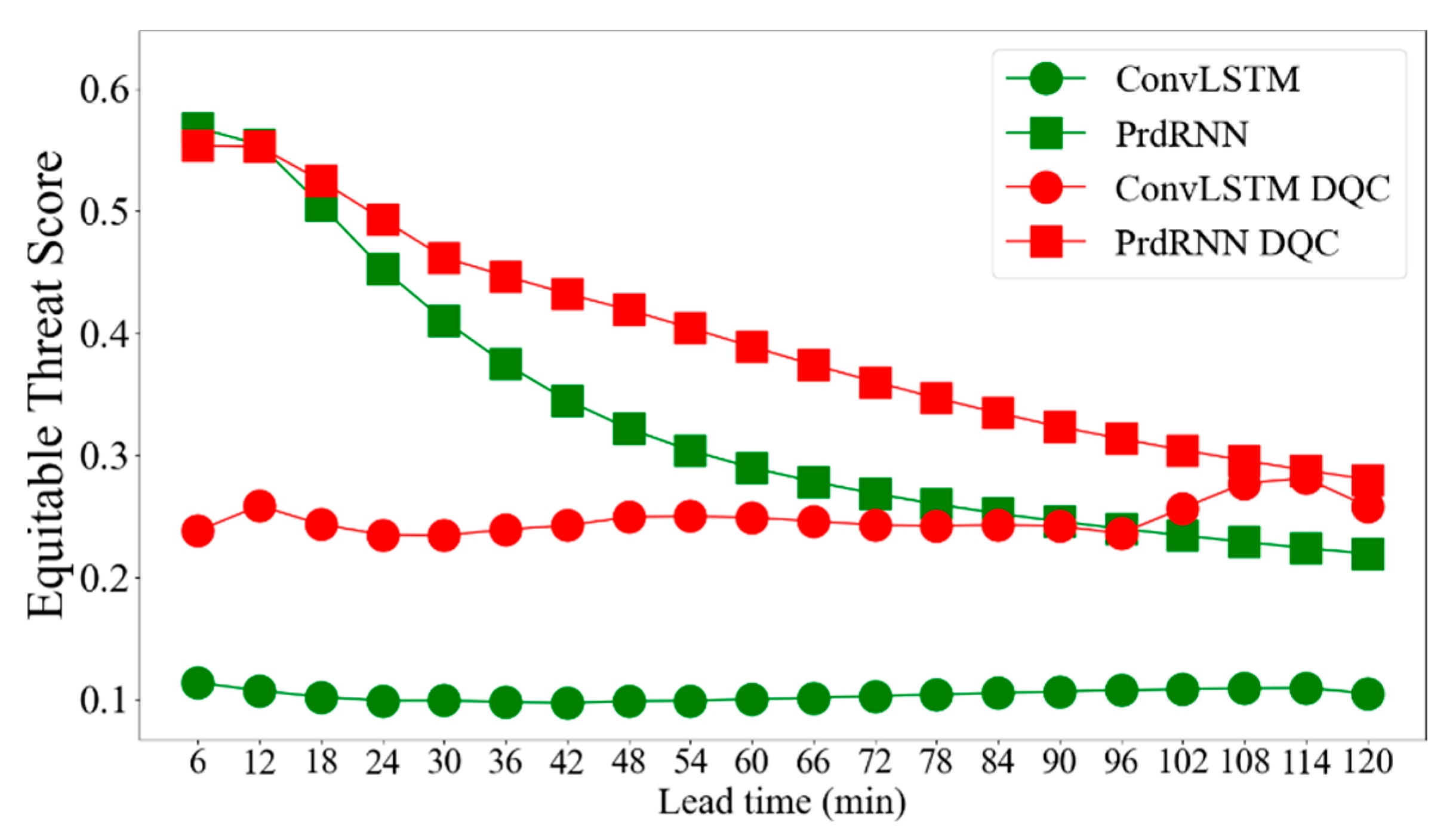
3.1. Data Quality Control (DQC) Evaluation

We selected May–September 2019 as the verification period because several extreme precipitation events occurred during this period. For example, intense rainstorms that occurred during 5–11 June 15–19 June, 20–25 June, and 27 June to 1 July caused notable geological and flood disasters [59].

Reducing the number of missing values in the original AWS data produced a complete time series and improved the spatial resolution of the dataset, thereby making the training samples more representative of the observed precipitation. Data normalization narrowed the range of extreme precipitation and improved the learning efficiency of the DL models with respect to the features of precipitation observations during the training process. Both processes helped DL models that exhibited improved performance in terms of ETS. The Hea-P dataset before and after data quality control (DQC) was divided into a training set and a validation set with a ratio of 8:1, and ETS evaluations were performed for the verification period.

The ETSs of the DL models for 6-min precipitation nowcasting before and after DQC are shown in Figure 2. The average ETS of the ConvLSTM model and of the PredRNN model increased by 0.1458 and 0.0660, respectively. The ConvLSTM model showed greater improvement in comparison with the PredRNN model; however, the PredRNN model also exhibited reasonable improvement beyond the 12-min lead time.

Currently, there is no unified evaluation metric for minute-level precipitation. Consequently, we calculated the ETS of hourly graded precipitation accumulated from 6-min precipitation for different thresholds (i.e., 0.1, 1, 2.5, 8, and 15 mm), as listed in

Table 1. ETSs of hourly graded precipitation for DL models before and after DQC for different thresholds (i.e., 0.1, 1, 2.5, 8, and 15 mm).

Model	ConvLSTM		ConvLSTM DQC		PredRNN		PredRNN DQC
Lead time	1 h	2 h	1 h	2 h	1 h	2 h	1 h	2 h
≥0.1 mm	0.1009	0.1658	0.3295	0.2523	0.4868	0.2121	0.5097	0.3425
≥1 mm	0.2223	0.1406	0.2637	0.2346	0.3574	0.1302	0.3694	0.2363
≥2.5 mm	0.1033	0.0922	0.0687	0.0390	0.2341	0.1046	0.3319	0.1700
≥8 mm	0.0039	0.0037	0.0032	0	0.0858	0.0276	0.1783	0.0586
≥15 mm	0	0	0.0004	0	0.1289	0.0283	0.2329	0.0594

. The forecasting skill of the ConvLSTM model with thresholds of 0.1 and 1 mm was well improved, and the ETS for the threshold of 0.1 mm for the 1-h lead time increased by 0.2286. Overall, the PredRNN model exhibited greater improvement in comparison with that of the ConvLSTM model, i.e., the average ETS for thresholds exceeding 2.5 mm for the 1-h lead time and for thresholds below 2.5 mm for the 2-h lead time increased by more than 0.09 and by 0.1305, respectively.

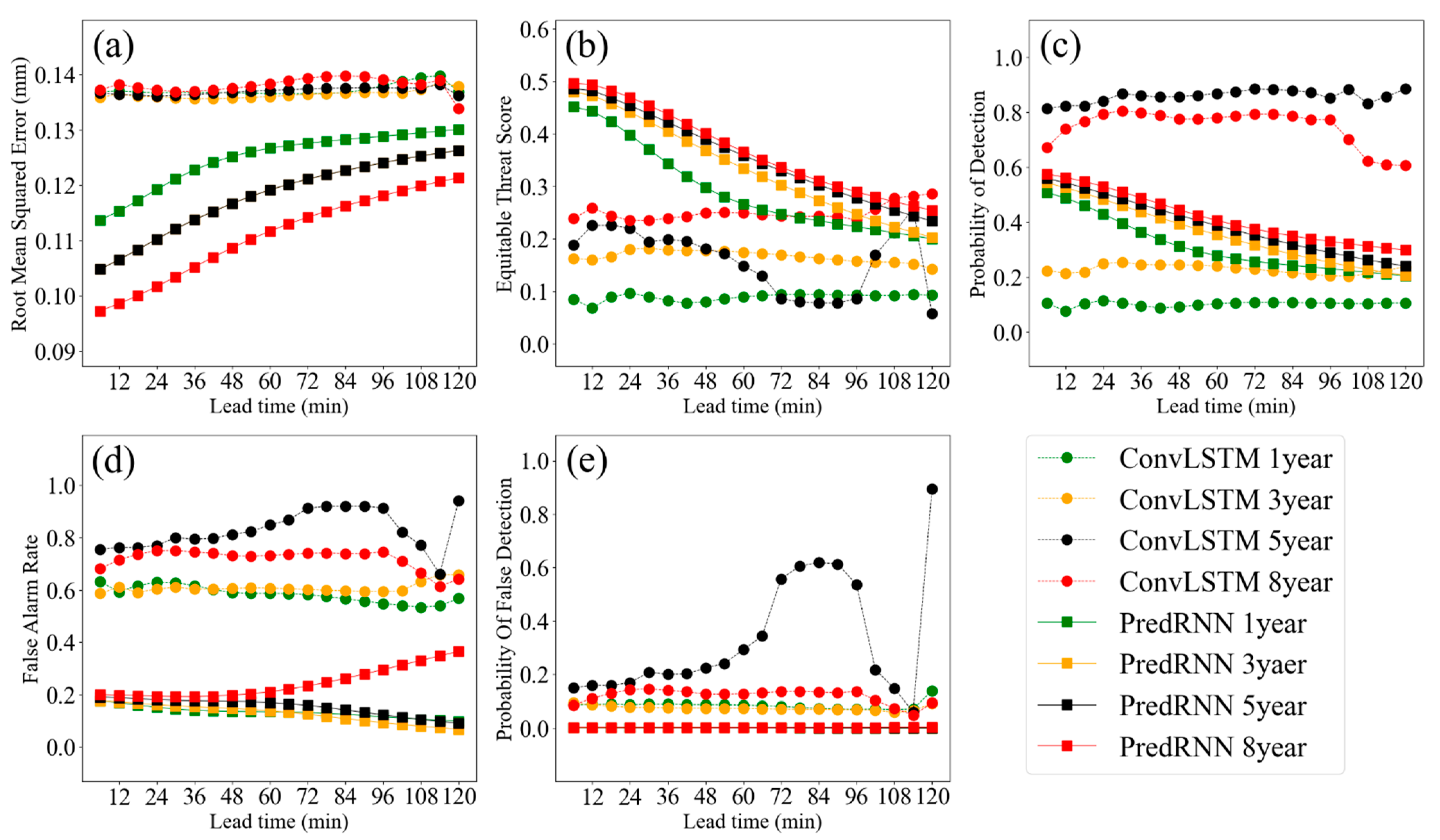
3.2. DL Models Trained Using Datasets with Different Time Series Lengths

Pre-P datasets with DQC and different time series lengths (i.e., 1, 3, 5, and 8 years) were divided into training sets, testing sets, and validation sets with ratios of 2:1:1, 6:1:1, 10:2:1, and 16:3:1, respectively, and the verification period for all evaluations was May–September 2019. Then, DL models were constructed using the training sets with different time series lengths (i.e., 1, 3, 5, and 8 years). Verifications including RMSE, ETS, POD, FAR, and POFD were applied to assess the 6-min precipitation nowcasting for the threshold of 0.01 mm generated using the DL models, as shown in Figure 3. With increasing length of the time series of the training set, the DL models showed a marked increase in terms of POD and ETS, and the stability of the nowcasts with time was enhanced, especially for the ConvLSTM model trained with the training set with the 8-year time series length, i.e., the average POD increased by 0.1066. Additionally, the PredRNN model trained with the training set with the 8-year time series length performed better than the ConvLSTM model, i.e., the RMSE decreased sharply, the FAR was low, and the ETS increased by 0.0763.

Taking the same verification period as above, we calculated the ETS of hourly graded precipitation (

Table 2. Hourly graded precipitation ETSs for the two DL models trained with Pre-P datasets with different time series lengths for different thresholds (i.e., 0.1, 1, 2.5, 8, and 15 mm).

Model	ConvLSTM 1 Year		ConvLSTM 3 Years		ConvLSTM 5 Years		ConvLSTM 8 Years
Lead time	1 h	2 h	1 h	2 h	1 h	2 h	1 h	2 h
≥0.1 mm	0.2553	0.0039	0.3015	0.0139	0.3232	0.3256	0.3295	0.2523
≥1 mm	0.2030	0.2113	0.2352	0.1300	0.2531	0.2534	0.2637	0.2346
≥2.5 mm	0.0135	0.0078	0.0313	0.0001	0.0170	0.0223	0.0687	0.0390
≥8 mm	0.0004	0	0.0067	0	0.0007	0.0013	0.0032	0
≥15 mm	0	0	0.0024	0	0	0.0006	0.0004	0
Model	PredRNN 1 Year		PredRNN 3 Years		PredRNN 5 Years		PredRNN 8 Years
Lead time	1 h	2 h	1 h	2 h	1 h	2 h	1 h	2 h
≥0.1 mm	0.4302	0.1257	0.4352	0.2455	0.4680	0.2560	0.4868	0.2121
≥1 mm	0.2991	0.0352	0.3112	0.1535	0.3468	0.1517	0.4183	0.1287
≥2.5 mm	0.0877	0.0211	0.1485	0.0209	0.1757	0.0389	0.2341	0.1046
≥8 mm	0.0011	0.0002	0.0062	0.0005	0.0122	0.0001	0.0858	0.0276
≥15 mm	0.0021	0.0003	0.0076	0.0028	0.0064	0.0025	0.1289	0.0283

). The ETSs of the DL models were improved with the increasing length of the time series of the training set. For the training set with the 8-year time series length, the ETS of the ConvLSTM model for the threshold of 0.1 mm increased sharply by 0.2484 for the 2-h lead time, while that for thresholds below 2.5 mm for the 1-h lead time increased by more than 0.05. However, the PredRNN model showed better improvement in terms of ETS. For example, the average ETS for the 0–2-h lead time for different thresholds (i.e., 0.1, 1, 2.5, 8, and 15 mm) increased by 0.0852, while that for the 1-h lead time increased by 0.1067, and that for the threshold of 2.5 mm increased by 0.1464.

To summarize, increasing the length of the training set time series and the number of the training samples both improved the forecasting skill of the DL models. Overall, the PredRNN model exhibited greater improvement in comparison with the ConvLSTM model, especially for the 1-h lead time, and the PredRNN model trained with the Pre-P dataset with the 8-year time series length obtained the best performance in terms of ETS.

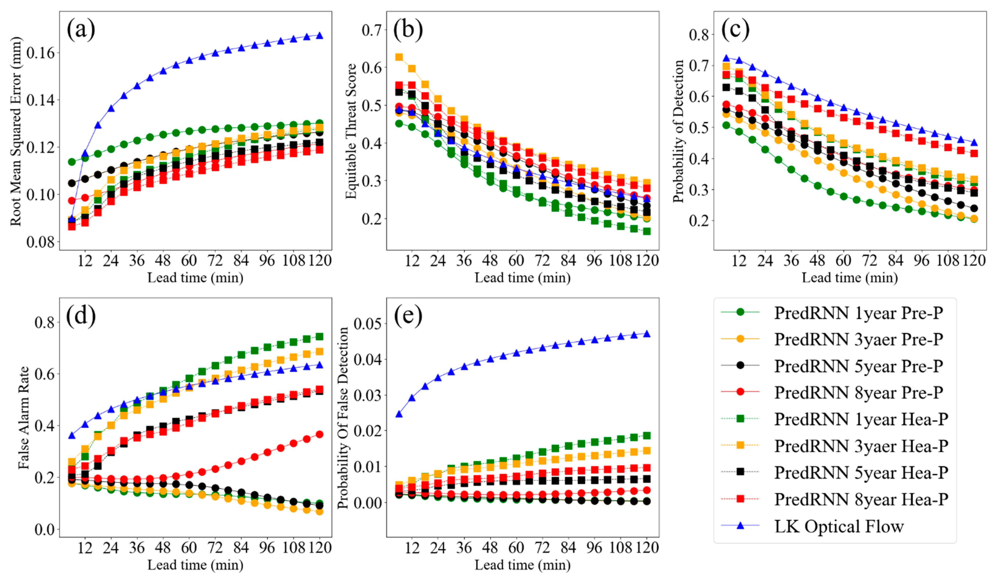
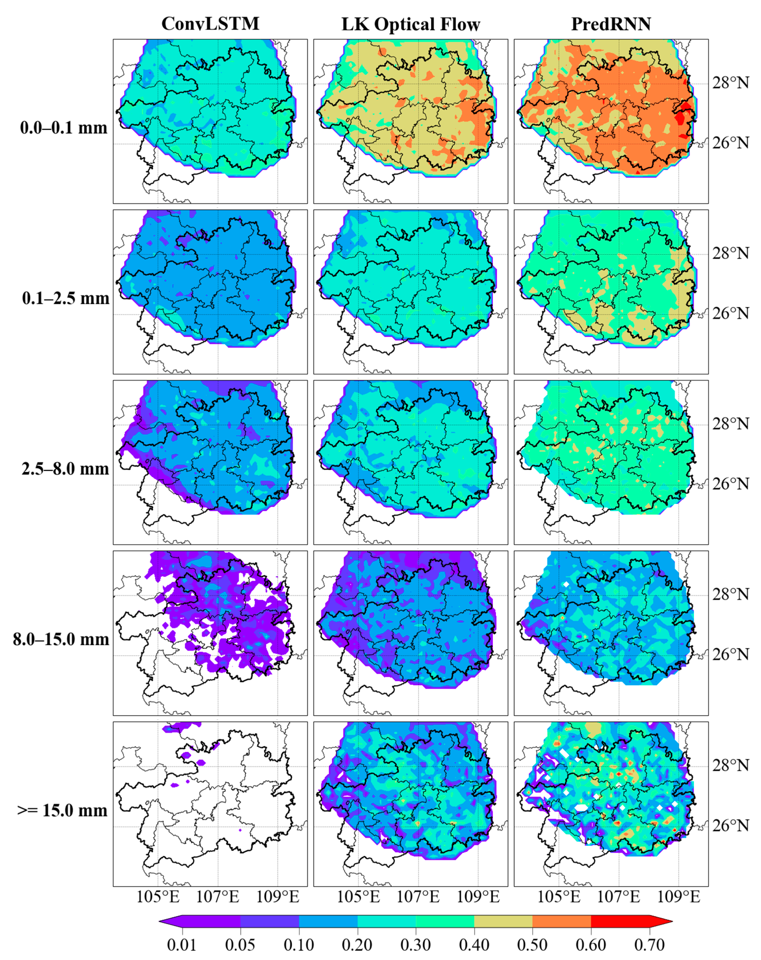
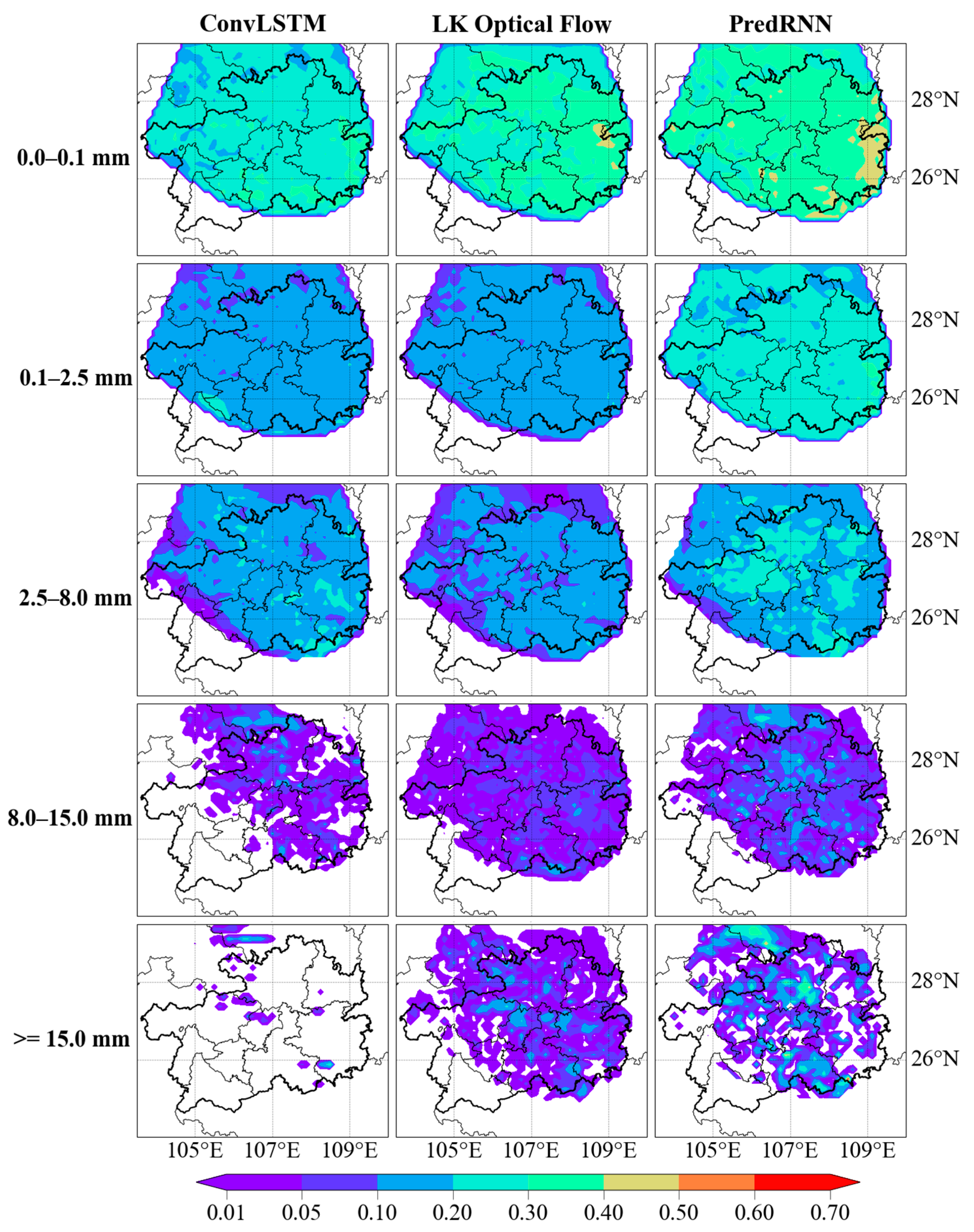
3.3. Deep Learning Model Training Using the Heavy Precipitation (Hea-P) Dataset

Although increasing the length of the time series of the training set could improve the forecasting skill of the DL models, the model with the best performance still exhibited no improvement in terms of the ETS for hourly graded precipitation when compared with the results obtained using the LK Optical Flow method (

Table 3. ETSs of hourly graded precipitation for the LK Optical Flow method and the DL models trained using the two types of datasets for different thresholds (i.e., 0.1, 1, 2.5, 8, and 15 mm).

Model	ConvLSTM 8 Years			PredRNN 8 Years			LK Optical Flow
Lead time	1 h	2 h	0–2 h	1 h	2 h	0–2 h	1 h	2 h	0–2 h
≥0.1 mm	0.3295	0.2523	0.2909	0.4868	0.2121	0.3495	0.4502	0.2914	0.3708
≥1 mm	0.2637	0.2346	0.2492	0.4183	0.1287	0.2735	0.3322	0.2011	0.2666
≥2.5 mm	0.0687	0.0390	0.0539	0.2341	0.1046	0.1694	0.2178	0.1061	0.1620
≥8 mm	0.0032	0.0000	0.0016	0.0858	0.0276	0.0567	0.1081	0.0422	0.0751
≥15 mm	0.0004	0.0000	0.0002	0.1289	0.0283	0.0786	0.1681	0.0407	0.1044

). Even though the ETS of the PredRNN model with the best performance was slightly higher than that of the traditional LK Optical Flow method for the thresholds of 0.1, 2.5, and 8.0 mm for the 1-h lead time, the ETS for the threshold of 15.0 mm for the 1-h lead time was lower than that derived using the LK Optical Flow method. Moreover, the ETSs of the PredRNN model with different thresholds (i.e., 0.1, 2.5, 8, and 15 mm) decreased rapidly with time, resulting in a lower overall ETS in comparison with that derived using the LK Optical Flow method.

To further improve the forecasting skill of the DL models, we removed samples with little or no precipitation and left the extreme precipitation to form the Hea-P dataset, which we hoped would represent a more effective training sample. Taking the same verification period as described in Section 3.2, Hea-P datasets with different time series lengths (i.e., 1, 3, 5, and 8 years) were divided into training sets, and validation sets with a ratio of 1:1, 3:1, 5:1, and 8:1, respectively. We constructed DL models using the training sets with time series of different lengths. Then, evaluation of the 6-min precipitation nowcasting was performed based on the RMSE, ETS, POD, FAR, and POFD, which allowed comparative assessment of the LK Optical Flow method and the DL models trained with the two types of datasets (i.e., Pre-P dataset and Hea-P dataset), as shown in Figure 4.

With a sharp increase in POD and reduction in RMSE for the 8-year time series length, the DL models trained with the Hea-P dataset performed better than those trained with the Pre-P dataset in terms of 6-min precipitation nowcasting; specifically, the PredRNN model outperformed the LK Optical Flow method in terms of forecasting skill. For the 1- and 3-year time series lengths, the DL models trained with the Hea-P dataset exhibited reduced ETSs and sharply increased FAR scores. Meanwhile, the DL models trained with the Hea-P datasets with the 5- and 8-year time series lengths also sharply increased in FAR scores. Overall, use of the Hea-P datasets improved the POD and resulted in sharply increased FAR values for the DL models because the DL models tended to generate more high-value precipitation nowcasting owing to training samples with high-value precipitation in the Hea-P dataset.

The ETSs of hourly graded precipitation for different thresholds are listed in

Table 4. ETSs of hourly graded precipitation for the PredRNN model trained with two types of datasets for different thresholds (i.e., 0.1, 1, 2.5, 8, and 15 mm).

Model		PredRNN 1 Year		PredRNN 3 Years		PredRNN 5 Years		PredRNN 8 Years
Pre-P dataset	Lead time	1 h	2 h	1 h	2 h	1 h	2 h	1 h	2 h
	≥0.1 mm	0.4302	0.1257	0.4352	0.2455	0.4680	0.2560	0.4868	0.2121
	≥1 mm	0.2991	0.0352	0.3112	0.1535	0.3468	0.1517	0.4183	0.1287
	≥2.5 mm	0.0877	0.0211	0.1485	0.0209	0.1757	0.0389	0.2341	0.1046
	≥8 mm	0.0011	0.0002	0.0062	0.0005	0.0122	0.0001	0.0858	0.0276
	≥15 mm	0.0021	0.0003	0.0076	0.0028	0.0064	0.0025	0.1289	0.0283
Hea-P dataset	Lead time	1 h	2 h	1 h	2 h	1 h	2 h	1 h	2 h
	≥0.1 mm	0.4612	0.2744	0.4492	0.2862	0.4743	0.3351	0.5097	0.3425
	≥1 mm	0.2571	0.1279	0.3168	0.1891	0.3513	0.2322	0.3694	0.2363
	≥2.5 mm	0.2498	0.1035	0.2506	0.0978	0.2664	0.1074	0.3319	0.1700
	≥8 mm	0.1320	0.0442	0.1334	0.0482	0.1384	0.0411	0.1783	0.0586
	≥15 mm	0.1177	0.0312	0.1774	0.0658	0.1828	0.0459	0.2329	0.0594

. The DL models trained with the Hea-P dataset improved markedly. The PredRNN model trained with the training set with the 8-year time series length obtained notable improvement for thresholds exceeding 2.5 mm, i.e., the ETS of the PredRNN model for thresholds of 2.5, 8, and 15 mm for a 1-h lead time increased sharply by 0.1141, 0.0702, and 0.0648, respectively. The average ETS for thresholds below 2.5 mm for the 2-h lead time also increased by more than 0.05. Importantly, the ETS for the threshold of 8.0 mm increased by an average of 0.0676 for a 0–2-h lead time and by 0.0925 for a 1-h lead time. Additionally, the ETS of the ConvLSTM model for the threshold of 2.5 mm increased by 0.0801, while that for below the threshold of 1.0 mm decreased (note: the ETSs of the ConvLSTM model are not listed in the table).

Comprehensive evaluation revealed the DL models with the performance in terms of ETS. The PredRNN model trained with the Hea-P dataset with the 8-year time series length obtained the best performance of all models in terms of ETS for hourly graded precipitation (

Table 5. ETSs of hourly graded precipitation for the LK Optical Flow method and the DL models trained with the Hea-P dataset for different thresholds (i.e., 0.1, 1, 2.5, 8, and 15 mm).

Model	ConvLSTM 8 Years		PredRNN 8 Years		LK Optical Flow
Lead time	1 h	2 h	1 h	2 h	1 h	2 h
≥0.1 mm	0.2526	0.2016	0.5097	0.3425	0.4502	0.2914
≥1 mm	0.1452	0.1108	0.3694	0.2363	0.3322	0.2011
≥2.5 mm	0.1337	0.1342	0.3319	0.1700	0.2178	0.1061
≥8 mm	0.0294	0.0283	0.1783	0.0586	0.1081	0.0422
≥15 mm	0.0012	0.0042	0.2329	0.0594	0.1681	0.0407

). The PredRNN model outperformed the LK Optical Flow method for all thresholds (i.e., 0.1, 1, 2.5, 8, and 15 mm), especially thresholds exceeding 2.5 mm. Although the ConvLSTM model was improved by training with the Hea-P dataset, it still performed a lower ETS than that of the other two models for all thresholds.

The spatial distributions of ETSs for hourly graded precipitation derived using the LK Optical Flow method and the DL models trained with the Hea-P dataset with the 8-year time series length for the 1-h lead time are shown in Figure 5. For thresholds of 0.1, 1, 2.5, and 8 mm, the higher the threshold, the lower the ETS of hourly graded precipitation; however, the ETS for the threshold of 8 mm exhibited a sharp decrease. Areas with high ETSs for thresholds of 0.1 and 1 mm mainly occurred in eastern, southern, and southwestern parts of Guizhou, whereas high ETSs for thresholds of 2.5, 8, and 15 mm mainly occurred in north-central and southern parts of Guizhou. For thresholds of 8 and 15 mm, the ETS of the ConvLSTM model was close to zero owing to many false predictions in areas of high-value precipitation and high values of POFD and FAR. This can result from cumulative error magnified by iterative calculation. For the threshold of 15 mm, the ETSs of the LK Optical Flow method and the PredRNN model showed improvement mainly in the southern and north-central parts of Guizhou. Additionally, the ETSs of the PredRNN model with different thresholds (i.e., 0.1, 1, 2.5, 8 and 15 mm) indicate that the PredRNN model outperformed both the ConvLSTM model and the LK Optical Flow method.

Figure 6 presents the spatial distributions of ETSs for the 2-h lead time. The ETSs of both the LK Optical Flow method and the PredRNN model for different thresholds (i.e., 0.1, 1, 2.5, 8, and 15 mm) decreased sharply for the 2-h lead time with the same pattern of spatial distribution as that shown for the 1-h lead time. The ETS of the PredRNN model for thresholds of 0.1 and 15 mm maintained values of 0.3–0.5 and 0.2–0.3, respectively, which were superior to the values of the other two models.

In summary, the DL models trained with the Hea-P dataset improved notably in terms of ETS for 6-min and hourly graded precipitation, especially for thresholds of 2.5, 8, and 15 mm. We determined that the PredRNN model trained with the Hea-P dataset with an 8-year time series length performed best, outperforming the LK Optical Flow method for all thresholds. Furthermore, it performed well for thresholds of 2.5, 8, and 15 mm in the north-central and southern parts of Guizhou.

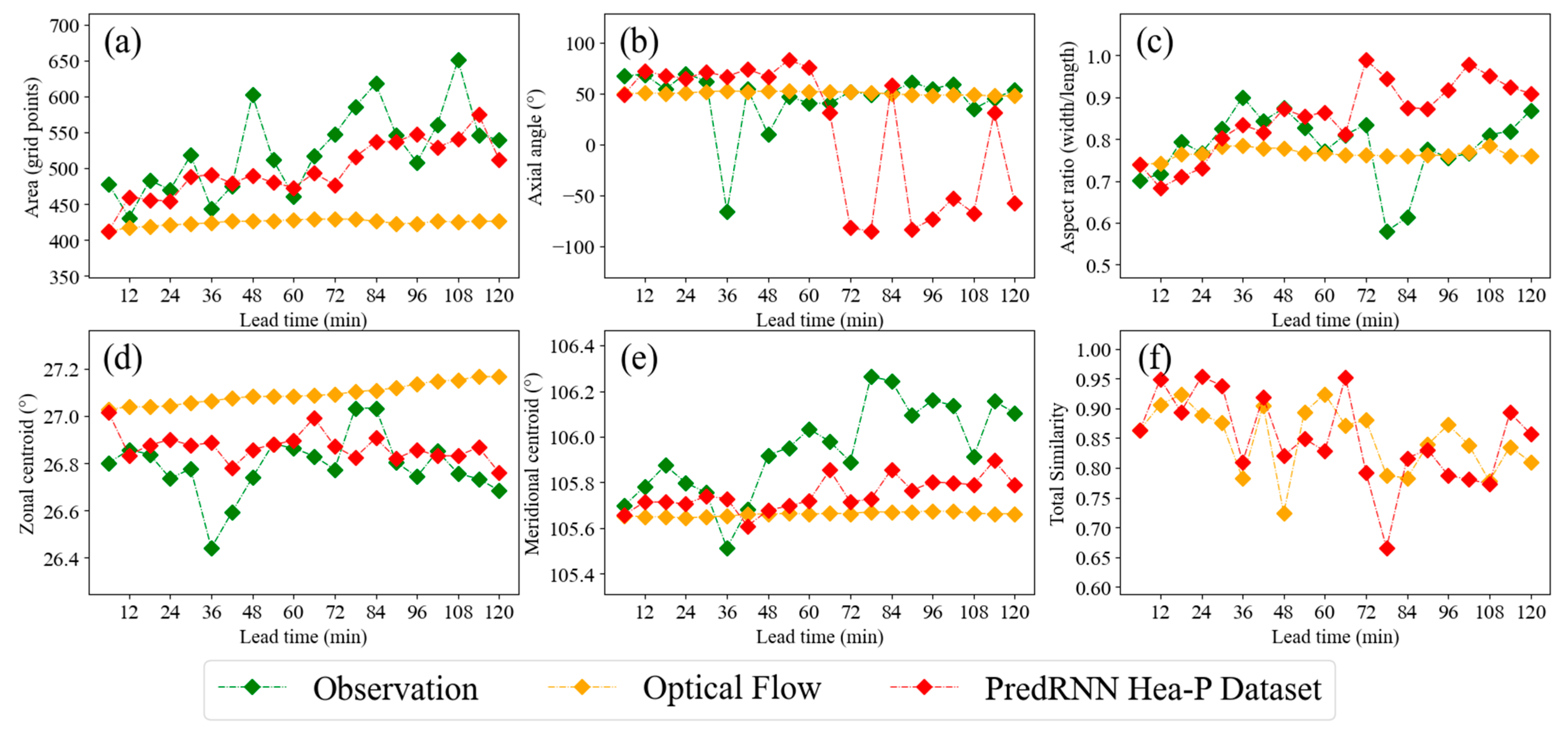
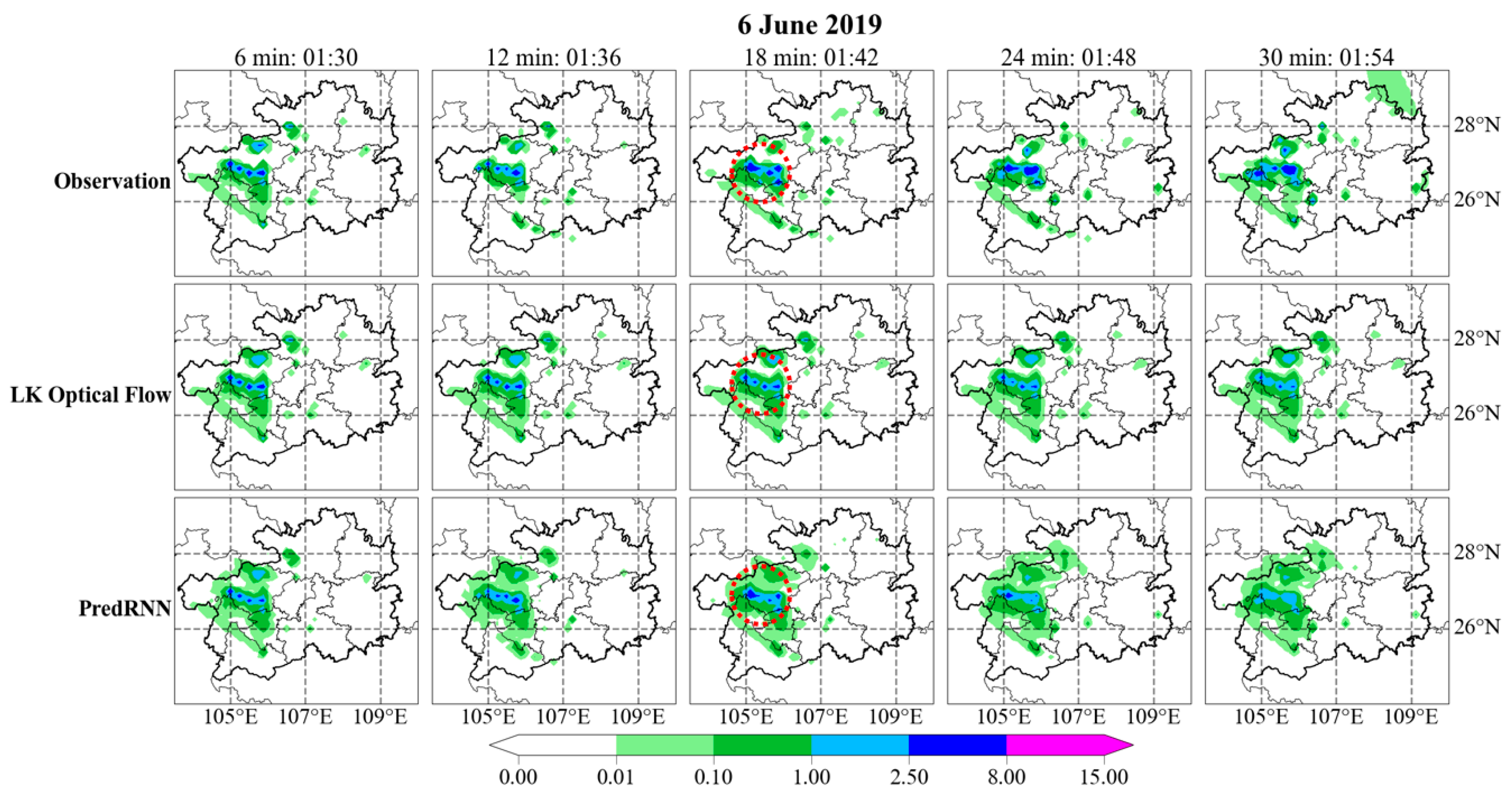
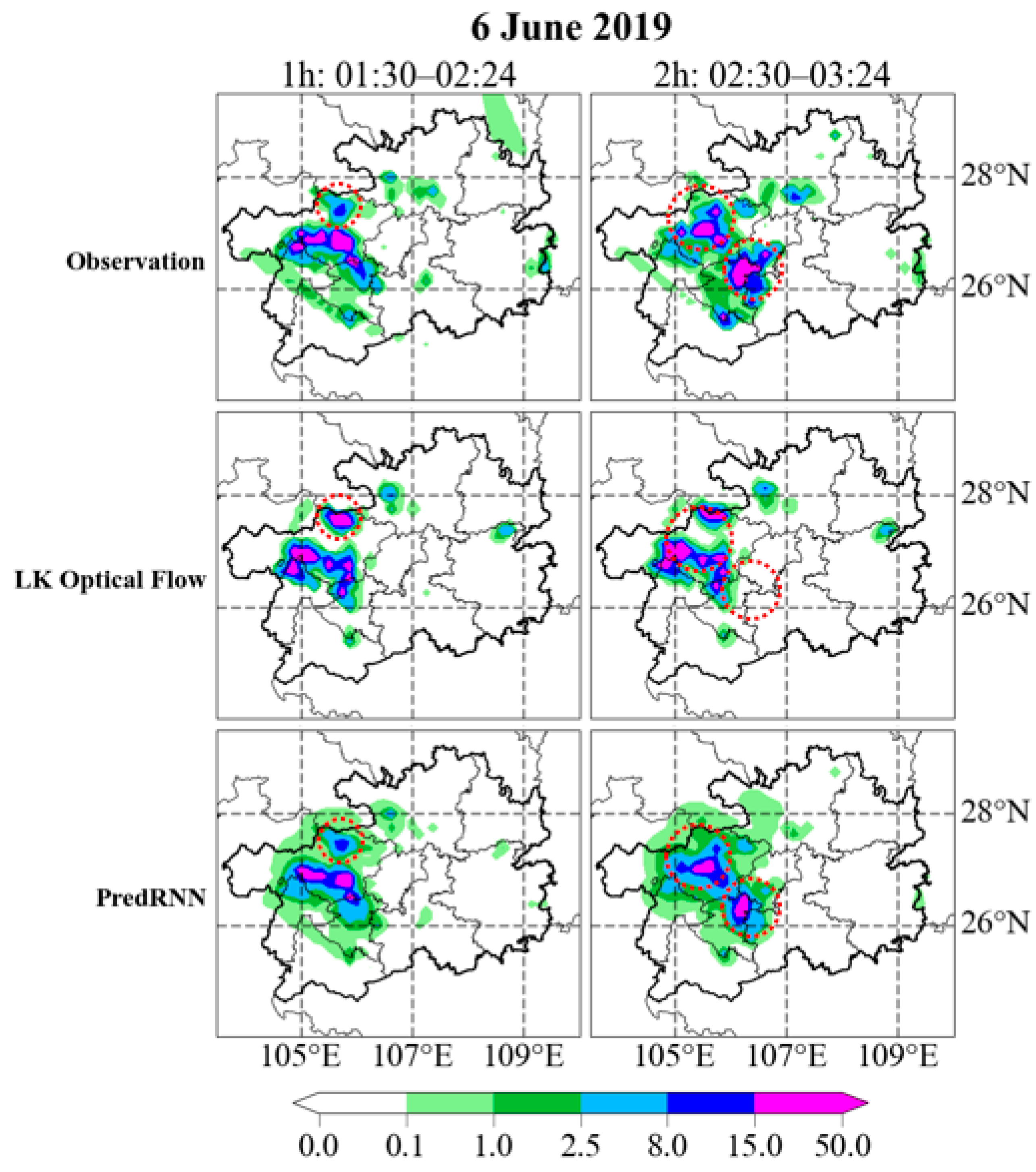
3.4. Structure Evaluation on a Rainstorm Case

As a case for evaluation, we selected a severe rainstorm event that occurred on 6 June 2019, which produced a two-hour period (01:30–03:24) of intense precipitation [59]. We used the MODE approach to further assess the performance of both the LK Optical Flow method and the PredRNN model trained with the Hea-P dataset with the 8-year time series length in relation to this rainstorm case. The MODE consisted of an evaluation of the 6-min precipitation for the threshold of 0.01 mm and an evaluation of the hourly graded precipitation for thresholds of 0.1, 1, and 2.5 mm.

The attribute values of the 6-min precipitation objects for the observations and nowcasts, calculated for a threshold of 0.01 mm, included the area, axis angle, aspect ratio, zonal centroid, and meridional centroid, from which we obtained the total similarity of the precipitation objects. All attribute values and the total similarity of the 6-min precipitation objects for both the LK Optical Flow method and the PredRNN model are shown in Figure 7. The attribute values of the observations have a wide range and show rapid fluctuation during the rainstorm, resulting in both the shape and the position of the area of precipitation varying wildly and rapidly with time. Meanwhile, the zonal centroid and the meridional centroid indicate that the precipitation system first evolved toward the southwest and then moved rapidly toward the northeast. With the characteristic of linear variation, the attribute values of the LK Optical Flow method change smoothly with time, whereas the attribute values of the PredRNN model fluctuate widely and are much closer to those of the observations.

It is evident from Figure 8 that the precipitation nowcasting of the LK Optical Flow method for 6–12-min lead times is highly similar to the observations and shows only minimal linear movement in position and shape. Nevertheless, with such characteristics, the deviation between the observations and the nowcasting of the LK Optical Flow method increases from 18 to 30 min. Conversely, the nowcasting generated using the PredRNN model for 18 to 30 min is closer to the observations because of the ability of the model to capture the nonlinear changes in the observations, demonstrating especially good performance for thresholds of 8 and 15 mm.

We calculated attribute values of hourly graded precipitation for thresholds of 0.1, 1, and 2.5 mm (

Table 6. Hourly graded precipitation MODE for different thresholds (i.e., 0.1, 1, and 2.5 mm) for the LK Optical Flow method and the PredRNN model trained with the Hea-P dataset with the 8-year time series length.

Precipitation Threshold	Observation or Forecast	Area (Grid Points)		Axial Angle (°)		Aspect Ratio (Width/Length)		Zonal Centroid (°)		Meridional Centroid (°)		Total Similarity
	Lead time	1 h	2 h	1 h	2 h	1 h	2 h	1 h	2 h	1 h	2 h	1 h	2 h
≥0.1 mm	Observation	474	499	47.98	50.59	0.73	0.81	26.79	26.78	105.86	106.04	—	—
	Optical Flow	372	377	65.17	64.77	0.72	0.74	26.94	27.03	105.67	105.68	0.85	0.81
	PredRNN	418	487	72.74	74.84	0.77	0.89	26.86	26.87	105.7	105.83	0.85	0.88
≥1 mm	Observation	178	265	30.47	−60.85	0.84	0.78	26.75	26.53	105.56	105.9	—	—
	Optical Flow	199	198	58.19	63.99	0.9	0.92	26.93	26.99	105.45	105.44	0.83	0.7
	PredRNN	175	205	41.36	−42.91	0.95	0.7	26.86	26.76	105.54	105.75	0.91	0.81
≥2.5 mm	Observation	105	150	21.5	−48.17	0.7	0.59	26.78	26.63	105.57	105.9	—	—
	Optical Flow	135	135	49.95	55.55	0.88	0.89	26.99	27.08	105.41	105.41	0.72	0.68
	PredRNN	92	123	20.11	−44.88	0.68	0.59	26.82	26.73	105.49	105.81	0.94	0.92

). The deviations between the observations and the nowcasting generated using the LK Optical Flow method are more pronounced for a 2-h lead time owing to the axial angle, aspect ratio, zonal centroid, and meridional centroid. Meanwhile, with an increase in the precipitation threshold, the PredRNN model trained with the Hea-P dataset with the 8-year time series length gradually increased in total similarity, substantially outperforming the LK Optical Flow method. For the threshold of 2.5 mm, the PredRNN model maintains a value of total similarity of >0.9, whereas the value for the LK Optical Flow method rapidly drops below 0.75.

The results of the above quantitative evaluation are well reflected in the spatial distributions of hourly precipitation shown in Figure 9. It is evident that the PredRNN model performs better than the LK Optical Flow method for thresholds exceeding 2.5 mm, i.e., it can well capture the nonlinear movement and evolution of the precipitation for a 2-h lead time. The LK Optical Flow method shows poor performance owing to the minimal changes in the shape and position of the area of precipitation with time, resulting in false predictions exceeding the threshold of 8.0 mm in northern Guizhou.

The characteristics of tiny movement and linear evolution mean that the precipitation nowcasting of the LK Optical Flow method is unable to capture nonlinear evolution that does not follow the rule of the latest optical flow vector in the observations. The errors also increased over time owing to the inability of the LK Optical Flow method to adapt to the rapid and extreme evolution of precipitation. However, the PredRNN model trained with the Hea-P dataset can overcome the deficiencies of the traditional LK Optical Flow method, capturing complex nonlinear evolution and establishing a reasonable mapping network during the drastic evolution of precipitation. Thus, the nowcasting of the PredRNN model is closer to the observations, especially for thresholds of 2.5, 8, and 15 mm.

4. Conclusions and Discussion

In this study, we formed two high-quality datasets (the Pre-P dataset and the Hea-P dataset) based on AWS precipitation observation data. Precipitation nowcasting at 6-min intervals for the lead times of 0–2 h was generated for Guizhou using the traditional LK Optical Flow method and the ConvLSTM and PredRNN DL models trained with the Pre-P and Hea-P datasets. Evaluations based on the RMSE, ETS, POD, and FAR were used to assess the performance of the different models in generating precipitation nowcasting. A rainstorm case was evaluated using the MODE approach to further examine the performance of the LK Optical Flow method and the PredRNN model trained with the Hea-P dataset with the 8-year time series length. The results obtained and the conclusions derived were as follows.

Reducing the number of missing values in the AWS observation data improved the quality of the DL training sample data. Data normalization also improved the training efficiency of the DL models. Both processes helped improve the forecasting skill of the DL models. The greater the length of the time series of the training dataset, the better the forecasting skill of the DL model. Increasing the time series length and the number of samples in the training data improved the POD and ETS of the DL models and enhanced the stability of the nowcasting over time. The PredRNN model was most improved for hourly graded precipitation, especially for the 1-h lead time.

Training with the Hea-P dataset further improved the forecasting skill of the DL models and sharply increased the ETSs for thresholds of 2.5, 8, and 15 mm, especially for the 1-h lead time. The improvement in the PredRNN model was greater than that in the ConvLSTM model. The PredRNN model trained with the Hea-P dataset with the 8-year time series length outperformed the traditional LK Optical Flow method for all thresholds (i.e., 0.1, 1, 2.5, 8, and 15 mm) and obtained the best performance in terms of ETS in comparison with the other DL models examined in this study. It also performed high ETSs for thresholds exceeding 2.5 mm in the north-central and southern parts of Guizhou. Additionally, the DL models tended to predict high-value precipitation owing to the high-value precipitation training samples in the Hea-P dataset, which is why most DL models showed a sharp increase in FAR values. The ETS of the ConvLSTM model for the threshold of 2.5 mm increased, but the ETS for the thresholds of 0.1 and 1 mm decreased owing to a sharp increase in the FAR. Owing to the magnified cumulative error through iterative calculation, the ConLSTM model performed many false predictions in high-value precipitation, and the ETS of the ConvLSTM model for thresholds of 8 and 15 mm was close to zero. Unlike radar data, observation instruments and measurement standards for precipitation observation data are unified in the industry. Generally, the spatial resolution of AWS data is higher than that of weather radar. Consequently, the DL models considered in this study could have reasonable transferability to other regions. Thus, the same approach could be used to construct highly accurate precipitation nowcasting DL models based on high-quality observation data.

The rainstorm case considered for evaluation revealed the characteristics of minimal movement and linear evolution in the traditional LK Optical Flow method. The generated precipitation nowcasting exhibited increasing error over time because the latest optical flow vector could not capture subsequent nonlinear evolution. Conversely, the PredRNN model trained with the Hea-P dataset could overcome the deficiencies of the traditional LK Optical Flow method and could capture the complex nonlinear evolution. Thus, the generated precipitation nowcasting was much closer to the observations. Specifically, the PredRNN model outperformed the traditional LK Optical Flow method for the threshold of 2.5 mm in the evaluated rainstorm case.

Currently, DL models using multisource observation data can overcome certain physical constraints and generate radar echoes that are physically more reasonable and of reference significance. For example, Li et al. [26] used a DL model and multisource data to produce radar echoes with physical characteristics that were improved in comparison with those derived using single-source observation data. In future work, DL models with multisource observations that include parameters such as temperature, pressure, and wind speed should be investigated. The inclusion of such dynamic and thermodynamic meteorological information will further improve the forecasting skill of DL models. Additionally, a comparative discussion with radar echo and more reasonable evaluation metrics will be added, such as radially averaged power spectral density [26,60,61].

References

1. Sun, J. Convective-scale assimilation of radar data: Progress and challenges. Q. J. R. Meteorol. Soc. 2005, 131, 3439–3463. [Google Scholar] [CrossRef]
2. Bachmann, K.; Keil, C.; Craig, G.C.; Weissmann, M.; Welzbacher, C.A. Predictability of deep convection in idealized and operational forecasts: Effects of radar data assimilation, orography, and synoptic weather regime. Mon. Weather Rev. 2020, 148, 63–81. [Google Scholar] [CrossRef]
3. Wang, T.; Liu, Y.; Dong, C.; Li, J. Review of short-term precipitation forecasting methods and their applications. Electron. World 2019, 10, 11–13. [Google Scholar]
4. Bowler, N.E.; Pierce, C.E.; Seed, A.W. STEPS: A probabilistic precipitation forecasting scheme which merges an extrapolation nowcast with downscaled NWP. Q. J. R. Meteorol. Soc. 2006, 132, 2127–2155. [Google Scholar] [CrossRef]
5. Pulkkinen, S. PySTEPS: An open-source Python library for probabilistic precipitation nowcasting (v1. 0). Geosci. Model Dev. 2019, 12, 4185–4219. [Google Scholar] [CrossRef]
6. Atencia, R.T.; Sairouni, A. Improving QPF by blending techniques at the meteorological service of catalonia. Nat. Hazards Earth Syst. Sci. 2010, 7, 1443–1455. [Google Scholar] [CrossRef]
7. Haiden, T.; Kann, A.; Wittmann, C.; Pistotnik, G.; Bica, B. The integrated nowcasting through comprehensive analysis (INCA) system and its validation over the eastern alpine region. Weather Forecast. 2011, 2, 166–183. [Google Scholar] [CrossRef]
8. Liang, Q.; Feng, Y.; Deng, W.; Hu, S.; Huang, Y.; Zeng, Q.; Chen, Z. A composite approach of radar echo extrapolation based on TREC vectors in combination with model predicted winds. Adv. Atmos. Sci. 2010, 5, 1119–1130. [Google Scholar] [CrossRef]
9. Sun, J.; Xue, M.; Wilson, J.W.; Zawadzki, I.; Ballard, S.P.; Onvlee-Hooimeyer, J.; Joe, P.; Barker, D.M.; Li, P.-W.; Golding, B.; et al. Use of NWP for nowcasting convective precipitation: Recent progress and challenges. Bull. Am. Meteorol. Soc. 2014, 95, 409–426. [Google Scholar] [CrossRef]
10. Ravuri, S.; Lenc, K.; Willson, M.; Kangin, D.; Lam, R.; Mirowski, P.; Fitzsimons, M.; Athanassiadou, M.; Kashem, S.; Madge, S.; et al. Skillful precipitation nowcasting using deep generative models of radar. Nature 2021, 597, 672–677. [Google Scholar] [CrossRef]
11. Crane, R.K. Automatic cell detection and tracking. IEEE Trans. Geosci. Electron. 1979, 17, 250–262. [Google Scholar] [CrossRef]
12. Rasmussen, R.; Dixon, M.; Hage, F.; Cole, J.; Rehak, N. Weather support to deicing decision making (WSDDM): A winter weather nowcasting system. Bull. Amer. Meteorol. Soc. 2001, 82, 579–596. [Google Scholar] [CrossRef]
13. Mueller, C.; Saxen, T.; Roberts, R.; Wilson, J.; Betancourt, T.; Dettling, S.; Oien, N.; Yee, J. NCAR auto-nowcast system. Weather Forecast. 2003, 18, 545–561. [Google Scholar] [CrossRef]
14. Cheung, P.; Yeung, H.Y. Application of optical-flow technique to significant convection nowcast for terminal areas in Hong Kong. In Proceedings of the 3rd WMO International Symposium on Nowcasting and Very Short-Range Forecasting (WSN12), Rio de Janeiro, Brazil, 6 August 2012; pp. 6–10. [Google Scholar]
15. Cao, C.Y.; Chen, Y.Z.; Liu, D.H. The optical flow method and its application to nowcasting. Acta Meteor. Sinica 2015, 73, 471–480. [Google Scholar]
16. Han, L.; Wang, H.Q.; Lin, Y.J. Application of optical flow method to nowcasting convective weather. Acta Sci. Nat. Univ. Pekin. 2008, 44, 751–755. [Google Scholar]
17. Feng, Y.; Kitzmiller, D. A short-range quantitative precipitation forecast algorithm using back-propagation neural network approach. Adv. Atmos. Sci. 2006, 23, 405–414. [Google Scholar] [CrossRef]
18. Dixon, M.; Wiener, G. TITAN: Thunderstorm identification, tracking, and nowcasting—A radar-based methodology. J. Atmos. Ocean. Technol. 1993, 10, 785–797. [Google Scholar] [CrossRef]
19. Johnson, J.T.; MacKeen, P.L.; Witt, A.; Mitchell, E.D.; Stumpf, G.J.; Eilts, M.D.; Thomas, K.W. The storm cell identification and tracking algorithm: An enhanced WSR-88D algorithm. Weather Forecast. 1998, 13, 263–276. [Google Scholar] [CrossRef]
20. Wilson, J.W.; Feng, Y.; Chen, M.; Roberts, R.D. Nowcasting challenges during the Beijing Olympics: Successes, failures, and implications for future nowcasting systems. Weather Forecast. 2010, 25, 1691–1714. [Google Scholar] [CrossRef]
21. LeCun, Y.; Bengio, Y.; Hinton, G. Deep learning. Nature 2015, 521, 436–444. [Google Scholar] [CrossRef]
22. Peng, T.; Zhi, X.; Ji, Y.; Ji, L.; Tian, Y. Prediction Skill of Extended Range 2-m Maximum Air Temperature Probabilistic Forecasts Using Machine Learning Post-Processing Methods. Atmosphere 2020, 11, 823. [Google Scholar] [CrossRef]
23. Zhu, Y.; Zhi, X.; Lyu, Y.; Zhu, S.; Tong, H.; Mamtimin, A.; Zhang, H.; Huo, W. Forecast calibrations of surface air temperature over Xinjiang based on U-net neural network. Front. Environ. Sci. 2022, 10, 2296–2665. [Google Scholar] [CrossRef]
24. Zhi, X.; Wang, J. Editorial: AI-based prediction of high-impact weather and climate extremes under global warming: A perspective from the large-scale circulations and teleconnections. Front. Earth Sci. 2023, 11, 2296–6463. [Google Scholar] [CrossRef]
25. Pan, X.; Lu, Y.; Zhao, K.; Huang, H.; Wang, M.; Chen, H. Improving Nowcasting of Convective Development by Incorporating Polarimetric Radar Variables Into a Deep-Learning Model. Geophys. Res. Lett. 2021, 48, e2021GL095302. [Google Scholar] [CrossRef]
26. Li, D.; Liu, Y.; Chen, C. MSDM v1.0: A machine learning model for precipitation nowcasting over eastern China using multisource data. Geosci. Model Dev. 2021, 14, 4019–4034. [Google Scholar] [CrossRef]
27. Shi, X.; Chen, Z.; Wang, H.; Yeung, D.Y.; Wong, W.K.; Woo, W.C. Convolutional LSTM network: A machine learning approach for precipitation nowcasting. Adv. Neural Inf. Process. Syst. 2015, 28, 1–12. [Google Scholar]
28. Shi, X.; Gao, Z.; Lausen, L.; Wang, H.; Yeung, D.Y.; Wong, W.K.; Woo, W.C. Deep learning for precipitation nowcasting: A benchmark and a new model. Adv. Neural Inf. Process. Syst. 2017, 30, 1–17. [Google Scholar]
29. Wang, Y.; Long, M.; Wang, J.; Gao, Z.; Yu, P.S. Predrnn: Recurrent neural networks for predictive learning using spatiotemporal lstms. Adv. Neural Inf. Process. Syst. 2017, 30, 1–10. [Google Scholar]
30. Wang, Y.; Gao, Z.; Long, M.; Wang, J.; Philip, S.Y. PredRNN++: Towards a resolution of the deep-in-time dilemma in spatiotemporal predictive learning. In Proceedings of the International Conference on Machine Learning, Stockholm, Sweden, 10–15 July 2018; pp. 5123–5132. [Google Scholar]
31. Ji, Y.; Gong, B.; Langguth, M.; Mozaffari, A.; Zhi, X. CLGAN: A GAN-based video prediction model for precipitation nowcasting. EGUsphere 2022, 1–23. [Google Scholar] [CrossRef]
32. Chen, X.; Liu, J.; Zheng, Q.; Li, X.; Liu, J. A Study on Radar Echo Nowcasting Based on Convolutional Gated Recurrent Unit Neural Network. Plateau Meteorol. 2021, 40, 1–13. [Google Scholar]
33. Foresti, L.; Sideris, I.; Nerini, D.; Beusch, L.; Germann, U. Using a 10-year radar archive for nowcasting precipitation growth and decay: A probabilistic machine learning approach. Weather Forecast. 2017, 34, 1547–1569. [Google Scholar] [CrossRef]
34. Agrawal, S.; Barrington, L.; Bromberg, C.; Burge, J.; Gazen, C.; Hickey, J. Machine learning for precipitation nowcasting from radar images. arXiv 2019, arXiv:1912.12132. [Google Scholar]
35. Mao, Y.; Sorteberg, A. Improving Radar-Based Precipitation Nowcasts with Machine Learning Using an Approach Based on Random Forest. Weather Forecast 2020, 35, 2461–2478. [Google Scholar] [CrossRef]
36. Germann, U.; Zawadzki, I. Scale dependence of the predictability of precipitation from continental radar images. Part II: Probability forecasts. J. Appl. Meteorol. 2004, 43, 74–89. [Google Scholar] [CrossRef]
37. Sun, N.; Zhou, Z.; Li, Q.; Zhou, X. Spatiotemporal Prediction of Monthly Sea Subsurface Temperature Fields Using a 3D U-Net-Based Model. Remote Sens. 2022, 14, 4890. [Google Scholar] [CrossRef]
38. Trebing, K.; Stańczyk, T.; Mehrkanoon, S. SmaAt-UNet: Precipitation nowcasting using a small attention-UNet architecture. Pattern Recognit. Lett. 2021, 145, 178–186. [Google Scholar] [CrossRef]
39. Gong, B.; Langguth, M.; Ji, Y.; Mozaffari, A.; Stadtler, S.; Mache, K.; Schultz, M.G. Temperature forecasting by deep learning methods. Geosci. Model Dev. Discuss. 2022, 15, 8931–8956. [Google Scholar] [CrossRef]
40. Chkeir, S.; Anesiadou, A.; Mascitelli, A.; Biondi, R. Nowcasting extreme rain and extreme wind speed with machine learning techniques applied to different input datasets. Atmos. Res. 2022, 282, 106548. [Google Scholar] [CrossRef]
41. Huang, H.; Lin, L.; Tong, R.; Hu, H.; Zhang, Q.; Iwamoto, Y.; Han, X.; Chen, Y.W.; Wu, J. Unet 3+: A full-scale connected unet for medical image segmentation. In Proceedings of the ICASSP 2020–2020 IEEE International Conference on Acoustics, Speech and Signal Processing (ICASSP), Barcelona, Spain, 4–8 May 2020; pp. 1055–1059. [Google Scholar]
42. Akbari Asanjan, A.; Yang, T.; Hsu, K.; Sorooshian, S.; Lin, J.; Peng, Q. Short-term precipitation forecast based on the persian system and lstm recurrent neural networks. J. Geophys. Res. Atmos. 2018, 123, 12543–12563. [Google Scholar] [CrossRef]
43. Ayzel, G.; Heistermann, M.; Sorokinc, A.; Nikitinc, O.; Lukyanovacet, O. All convolutional neural networks for radar-based precipitation nowcasting. Procedia Comput. Sci. 2019, 150, 186–192. [Google Scholar] [CrossRef]
44. Su, A.; Li, H.; Cui, L.; Chen, Y. A convection nowcasting method based on machine learning. Adv. Meteorol. 2020, 2020, 5124274. [Google Scholar] [CrossRef]
45. Tian, L.; Li, X.; Ye, Y.; Xie, P.; Li, Y. A generative adversarial gated recurrent unit model for precipitation nowcasting. IEEE Geosci. Remote Sens. Lett. 2020, 17, 601–605. [Google Scholar] [CrossRef]
46. Han, L.; Sun, J.; Zhang, W. Convolutional neural network for convective storm nowcasting using 3-d doppler weather radar data. IEEE Trans. Geosci. Remote Sens. 2019, 58, 1487–1495. [Google Scholar] [CrossRef]
47. Suzanna, M.; Alexandre, E. Precipitation Nowcasting with Weather Radar Images and Deep Learning in São Paulo, Brasil. Atmosphere 2020, 11, 1157. [Google Scholar]
48. Yu, L.; Du, X.; Zhao, L.; Yang, H. A new methodology for pixel-quantitative precipitation nowcasting using a pyramid Lucas Kanade optical flow approach. J. Hydrol. 2015, 529, 354–364. [Google Scholar]
49. Gan, W.; Li, G.; Wan, X. Variation Characteristics of Extreme Precipitation During May-September in Guizhou Province in Recent 57 Years. J. Arid. Meteorol. 2018, 36, 617–623. [Google Scholar]
50. Bai, H.; Gao, H. Influences of the Somaliacross-equatorial flow on the beginning date of rainy season in Southwest China. Chin. J. Atmos. Sci. 2017, 41, 702–712. (In Chinese) [Google Scholar]
51. Reich, S. An explicit and conservative remapping strategy for semi-Lagrangian advection. Atmos. Sci. Lett. 2017, 8, 58–63. [Google Scholar] [CrossRef]
52. Zhu, S.; Zhang, L.; Jiang, H.; Lyu, Y.; Fan, Y.; Guo, Z.; Zhi, X. Pattern projection calibrations on subseasonal forecasts of surface air temperature over East Asia. Weather. Forecast. 2023. [Google Scholar] [CrossRef]
53. Zhu, S.; Zhi, X.; Ge, F.; Fan, Y.; Zhang, L.; Gao, J. Subseasonal forecast of surface air temperature using superensemble approaches: Experiments over Northeast Asia for 2018. Weather. Forecast. 2021, 36, 39–51. [Google Scholar] [CrossRef]
54. Lyu, Y.; Zhi, X.; Zhu, S.; Fan, Y.; Pan, M. Statistical calibrations of surface air temperature forecasts over East Asia using pattern projection methods. Weather. Forecast. 2021, 36, 1661–1674. [Google Scholar] [CrossRef]
55. Davis, C.; Brown, B.; Bullock, R. Object-based verification of precipitation forecasts. Part I: Methodology and application to mesoscale rain areas. Mon. Weather Rev. 2006, 134, 1772–1784. [Google Scholar] [CrossRef]
56. Davis, C.; Brown, B.; Bullock, R. Object-based verification of precipitation forecasts. Part II: Application to convective rain systems. Mon. Weather Rev. 2006, 134, 1785–1795. [Google Scholar] [CrossRef]
57. Johnson, A.; Wang, X. Object-Based Evaluation of a Storm-Scale Ensemble during the 2009 NOAA Hazardous Weather Testbed Spring Experiment. Mon. Weather Rev. 2013, 141, 1079–1098. [Google Scholar] [CrossRef]
58. Ji, L.; Zhi, X.; Simmer, C.; Zhu, S.; Ji, Y. Multimodel ensemble forecasts of precipitation based on an object-based diagnostic evaluation. Mon. Weather Rev. 2020, 148, 2591–2606. [Google Scholar] [CrossRef]
59. Min, A.; Liao, Y.; Deng, W.; Zhang, C. A brief description of the main rainstorm weather process in China from April to October 2019. Torrential Rain Disasters 2020, 39, 539–548. [Google Scholar]
60. Ayzel, G.; Scheffer, T.; Heistermann, M. RainNet v1.0: A convolutional neural network for radar-based precipitation nowcasting. Geosci. Model Dev. 2020, 13, 2631–2644. [Google Scholar] [CrossRef]
61. Huang, Q.; Chen, S.; Tan, J. TSRC: A Deep Learning Model for Precipitation Short-Term Forecasting over China Using Radar Echo Data. Remote Sens. 2022, 15, 142. [Google Scholar] [CrossRef]
Figure 1. Distribution of the 1835 automatic weather stations in Guizhou Province, China.
Atmosphere 14 00807 g001
Figure 2. Comparison of the ETSs of the DL models before and after data quality control (DQC).
Atmosphere 14 00807 g002
Figure 3. Forecasting skill of DL models trained with different time series lengths: (a) RMSE, (b) ETS, (c) POD, (d) FAR, and (e) POFD.
Atmosphere 14 00807 g003
Figure 4. Forecasting skill of the LK Optical Flow model and the PredRNN model trained with two types of datasets: (a) RMSE, (b) ETS, (c) POD, (d) FAR, and (e) POFD.
Atmosphere 14 00807 g004
Figure 5. Spatial distributions of ETSs for hourly graded precipitation for the 1-h lead time, derived from the LK Optical Flow method and the DL models trained with the Hea-P dataset with the 8-year time series length.
Atmosphere 14 00807 g005
Figure 6. Spatial distributions of ETSs for hourly graded precipitation for the 2-h lead time, derived from the LK Optical Flow method and the DL models trained with the Hea-P dataset with the 8-year time series length.
Atmosphere 14 00807 g006
Figure 7. Attribute values of 6-min precipitation objects for the LK Optical Flow method and the PredRNN model trained with the Hea-P dataset with the 8-year time series length: (a) area, (b) axis angle, (c) aspect ratio, (d) zonal centroid, (e) meridional centroid, and (f) total similarity.
Atmosphere 14 00807 g007
Figure 8. Distributions of observed and predicted precipitation for 6–30-min lead times for the evaluated rainstorm case.
Atmosphere 14 00807 g008
Figure 9. Distributions of observed and predicted hourly precipitation for 6–30 min lead times for the evaluated rainstorm case.
Atmosphere 14 00807 g009