Article

Impacts of Complex Terrain Features on Local Wind Field and PM2.5 Concentration

1
Dalian Meteorological Observatory, Dalian 116000, China
2
School of Environment, Nanjing Normal University, Nanjing 210046, China
*
Author to whom correspondence should be addressed.
Atmosphere 2023, 14(5), 761; https://doi.org/10.3390/atmos14050761
Submission received: 12 February 2023 / Revised: 13 April 2023 / Accepted: 20 April 2023 / Published: 22 April 2023

Abstract

:
Complex topography has nonnegligible effects on local meteorological conditions as well as the transportation of atmospheric pollutants, which deserves more extensive study. In this study, the impacts of complex terrain features (mountains and river valleys) on local wind field and PM2.5 concentration in a typically developed mega city along the Yangtze River were studied numerically using the WRFCALMET-CALPUFF system. The impacts of different model grid and terrain horizontal resolutions were firstly investigated against observations. Then, the impacts of terrain features, specifically the impacts of Mt. LS and the Yangtze River, on wind field and PM2.5 transportation were analyzed by “removing” Mt. LS and the Yangtze River from the meteorological diagnostic model and simulating the dispersion of PM2.5 from three virtual point sources in the chemical model. Results showed that: (i) higher terrain elevation and model horizontal resolutions, and updated land cover types, can effectively improve the prediction of wind direction where terrain features are complex; (ii) Mt. LS mainly acts as a barrier, and ridge wind is weakened after “removing” Mt. LS; (iii) after “removing” the Yangtze River, the transport of PM2.5 along the Yangtze River is weakened; (iv) the simulation of PM2.5 from virtual point sources showed that Mt. LS could have an effect of up to 55% on the PM2.5 concentration in Nanjing. This study showed that the local complex topographies have an obvious effect on the local wind field and the concentration of PM2.5. Therefore, it is important to consider the influence of local topographies and land cover types when predicting local wind field and air quality.

1. Introduction

Due to rapid development, air pollution has attracted more public attention [1,2]. Frequent haze pollution is closely related to adverse meteorological conditions and high pollutant emissions [3,4,5,6]. Evidence has shown that air quality in China has been improved a lot owing to the large decrease in anthropogenic emissions, and meteorological conditions are recently becoming key factors on air quality [7,8]. Severe air pollution characterized by high concentrations of PM2.5 can occur more frequently over complex terrains even with relatively weak anthropogenic emissions, due to comprehensive impacts of underlying features on planetary boundary layer (PBL) conditions [9]. In addition, new particles may form under different levels of air pollutants combined with meteorological effects [10]. Therefore, it is important to study quantitatively the impacts of complex terrain features on the transportation and distribution of air pollutants.
Meteorological conditions in the PBL are the main factors affecting air quality, especially near-surface meteorological elements, such as wind speed, wind direction, relative humidity, temperature, and mixed-layer thickness, which have a direct influence on the diffusion and transport of pollutants in the PBL [11]. Among all those meteorological factors, wind speed and wind direction affect pollutants more frequently. Complex terrains usually exhibit complex effects (dynamically and thermally) on local wind fields; therefore, local air quality can also be affected. Pollution is often accompanied by weak near-surface wind which could lead to the accumulation of pollutants, while wind direction determines the transmission and diffusion of pollutants [12,13]. Over complex terrains with mountains, valleys, and multiple land covers, wind speed and wind direction in the PBL are strongly affected by dynamical and thermal processes (non-geostrophic winds are usually formed), thus weakening/strengthening the ability of the atmosphere to remove local atmospheric pollutants [14,15]. However, current quantitative analysis of how complex terrains affect local wind field and air quality is still insufficient, and numerical simulation results often have large errors due to the insufficient representation of local terrain features.
Due to the temporal and spatial limitations of the observation data, numerical models have become a widely used method to study the diffusion and transport of pollutants under complex topographies. Most studies focus on the analysis of the atmospheric boundary layer structure under different pollution processes [16] and the impacts of different boundary layer parameterization schemes [17,18]. However, it is difficult for numerical models to accurately capture the atmospheric boundary layer structure and wind field over complex topographies due to the parameterized turbulence calculation in the PBL. For example, the Weather Research and Forecasting (WRF) model usually overestimates near-surface wind speed [19,20], which could be due to the difficulty in accurately describing surface roughness under complex topographies [21]. In addition, horizontal and vertical grid resolutions also affect the simulation of near-surface wind [22]. Studies have shown that it is difficult to simulate the wind profile with WRF below 100 m [22], and large wind direction errors often occur when the wind speed is low [23]. The bias of wind simulation under complex topographies can be reduced when a large-eddy simulation is introduced [9]. However, such a procedure not only requires more accurate topographic information and more detailed land cover types [24,25], but also needs large computational resources. In recent years, the coupling of mesoscale models and small regional models has been widely used in near-surface wind field simulation. For example, studies have shown that the coupling of WRF and CALMET (the meteorological diagnosing part of the air quality dispersion model CALPUFF) can better simulate near-surface wind fields [26]. Furthermore, such a procedure could save lots of computational resources compared to large-eddy simulation.
Nanjing, one of the largest developed cities in China, is located on the east coast of the middle latitude continent and the lower reaches of the Yangtze River. The widest part of the Yangtze River in Nanjing can reach 2 km, and the Ningzhen Mountains and Mt. LaoShan (LS) are located along the Yangtze River as shown in Figure 1. The average altitude of Mt. LS is about 200 m, and the highest peak is 442 m. Due to large anthropogenic emissions, it is of great scientific significance to study the diffusion and transmission law of pollutants under complex topographies to improve the air quality of Nanjing and maintain the coordinated development of environment and economy. Based on meteorological observations during 2017–2019 in Nanjing, it is found that the dominant wind direction of the Pukou Station (PK) in Nanjing is very different from that of the other station (Figure 1a,b). By comparing the hourly observation data of the PK and the Liuhe Station (LH) in Nanjing from 2017 to 2019, it is found that a wind direction difference of greater than 90° and between 45° and 90° accounted for 13.5% and 17.9%, respectively. The difference in wind direction between the two stations is probably due to the complex terrain features. Therefore, in order to accurately simulate the wind field and the transport and diffusion of PM2.5 in Nanjing, the impacts of model grid and terrain height data resolutions, land cover types, and the Mount LS and Yangtze River topographies are studied in this study.
The aim of the study is to discuss the impacts of different model grid and topographic elevation resolutions, and land cover types, on local wind field simulation as well as the transport and distribution of PM2.5. In this manuscript, data and the model configurations are described in Section 2. Then, the model performances with different configurations are evaluated in Section 3.1, and the impacts of complex terrain features on local wind field and the distribution of PM2.5 concentration are discussed in Section 3.2 and Section 3.3. Conclusions are made in Section 4.

2. Data and Methods

2.1. Data

The meteorological observation data used in this study are the hourly observation data of wind speed and direction from the national meteorological stations PK (118.62° E, 32.05° N) and LH (118.83° E, 32.35° N) in Nanjing, obtained from the China Meteorological Data Service Centre of the National Meteorological Information Centre as shown in Figure 1, which is also used to evaluate the model performance. The wind observations were measured at 10 m above the ground using a ZQZ-TFR wind sensor, which has a sampling frequency of 1 s−1; the sampling accuracy is 0.1 m s−1 and 0.01° for wind speed and wind direction, respectively.
The initial and boundary conditions for WRF simulation are provided by the Global Data Assimilation System with a horizontal resolution of 0.25°and a temporal resolution of 6 h. The topography height data used in WRF and CALMET are updated using the Shuttle Radar Topography Mission (SRTM-3) with a horizontal resolution of approximately 100 m. In addition, the symbols and units used in the manuscript are shown in Table S3.

2.2. Model Configurations

In this study, WRF version 4.2, jointly developed by the National Centers for Environmental Prediction (NCEP), the National Center for Atmospheric Research (NCAR), and other departments [27], was used to generate the first meteorological guesses for the CALMET diagnostic model. CALMET is a meteorological module of the unsteady Lagrange model CALPUFF for downscale analysis, which includes a diagnostic wind field generator containing objective analysis and parameterized treatments of slope flows, kinematic terrain effects, terrain blocking effects, a divergence minimization procedure, and a micro-meteorological model for overland and overwater boundary layers. Configurations of WRF are shown in Table 1. Firstly, two sets of WRF simulations, namely the WRF1000 (the innermost domain has a horizontal resolution of 1 km) and WRF300 (the innermost domain has a horizontal resolution of 300 m), are configured with three layers of grid nesting with different horizontal resolutions. For WRF300, topographic correction for surface winds to represent extra drag from sub-grid topography and enhanced flow at hill tops is turned on (topo_wind = 1). The outermost grid covers the Yangtze River Delta and its surrounding areas, and the innermost grid covers the entire study area.
The innermost results of the WRF simulations were then used as first guesses for the CALMET model for further meteorological field downscaling. The simulation region of CALMET is shown in Figure 1c with a horizontal resolution of 150 m and 25 unevenly distributed vertical layers from near ground to 2000 m (with a resolution of 20 m below 200 m). In order to optimize the wind simulation, three WRF-CALMET simulations with different first guesses and land-use types (LU) were configured, namely WRF1000-CALMET150, WRF300-CALMET150, and WRF300-CALMET150-LU. The WRF1000-CALMET150 and WRF300-CALMET150 experiments used WRF default USGS land cover types (1999 version), while WRF300-CALMET150-LU updated the land cover types to 2021 based on the 30 m resolution land cover data of China developed by Yang and Huang [28], and the relevant parameters of different land cover types were updated correspondingly. The modified parameters include: surface roughness, albedo, Bowen ratio, soil heat flux parameter, and leaf area index.
In addition, in order to reflect the influence of local topographies on wind field and the distribution of PM2.5 concentration, the Yangtze River and Mount LS within the study area were respectively “removed” in some simulations (for LS, the terrain height of grids within the LS region was reduced to 10 m, so that Mt. LS became a flat region; for the Yangtze River, the terrain heights of grids within the Yangtze River and its coastal areas were all set to 10 m, and the land type was changed to built-up land). Three virtual emission point sources (located in the Jiangbei Chemical Industry Park, Qixia District, and Gulou District, respectively, as shown in Figure 1c) were respectively configured to test the transport and diffusion of PM2.5. The base height, stack elevation, exit diameter, exit velocity, exit temperature, and emission rate were 50 m, 5 m, 3 m, 10 m s−1, 363 K, and 1000 tons per year, respectively. CALPUFF was adopted to simulate PM2.5 transport and diffusion, and eight groups of experiments were set up. The descriptions of each experiment are shown in Table 2. In this study, January, April, July, and October of 2019 were selected as simulation periods, representing winter, spring, summer, and autumn, respectively. Another group of experiments was conducted to compare the dispersion forecasts by using the WRF1000 and WRF300_CALMET150 meteorology, which also recommends higher precision simulation (Text S3 and Figure S4).

3. Results and Discussion

3.1. Comparative Analysis of Downscaled Wind Field from Different Experiments

As the PK station is located within Mt. LS, and the dominant wind direction is quite different from the other station in Nanjing, the simulated wind at PK was compared with observations to evaluate the model’s performance. The comparisons between hourly simulated wind speed and observed wind speed at the PK station in different experiments are shown in Figure 2. In general, increasing horizontal resolutions and the precision of the underlying surface do not significantly improve the simulation of wind speed, and CALMET generally performs better than WRF. The root-mean-square error (RMSE) of wind speed of WRF1000_CALMET150 fluctuates in the range of 1.03–1.23 m/s. However, the RMSE of wind speed fluctuates in the range of 1.57–3.72 m/s and 1.64–3.72 m/s after the improvement of horizontal resolution (WRF300_CALMET150) and underlying surface precision (WRF300_CALMET150_LU), respectively. Meanwhile, the correlation coefficients between simulated wind speed and observed wind speed in the three experiments are 0.47–0.65, 0.21–0.54, and 0.21–0.54.
The evaluation results of wind direction are shown in Table 3, Text S2 and Figure S3. It indicates that improving the model horizontal resolution, topographic elevation, and land cover types can significantly improve the simulation of wind direction. The RMSE of wind direction in WRF1000_CALMET150 fluctuates in the range of 102.7–166.6°, while those in WRF300_CALMET150 and WRF300_CALMET150_LU fluctuate in the range of 59.6–77.6° and 56.0–71.6°. Meanwhile, compared with WRF1000_CALMET150, the absolute biases (Abias) of WRF300_CALMET150 and WRF300_CALMET150_LU are reduced by 33.3–60.5% and 35.9–66.1%, respectively. These promising results showed that the resolutions of model grids and topographic elevation are critical to the simulation of wind direction, especially over regions with complex terrains. This is because WRF is a mesoscale model which can hardly deal with small-scale features, such as PBL turbulence, slope wind, etc., unless with the use of the large-eddy simulation. However, CALMET is a diagnostic model with advanced abilities describing small-scale features; therefore, CALMET is expected to be better than WRF in wind field simulation. For terrains that are relatively flat, further improvement of WRF grid resolution did not show much positive effect on wind simulation (Tables S1 and S2). This is because the theoretical finest horizontal resolution to use PBL parameterizations is 1 km. Further improvement of horizontal resolution could cause unrecognized bias. In addition, these similar statistics for the LH station are shown in Text S4, Tables S1 and S2.

3.2. Influences of Different Topographies

As discussed above, increasing the horizontal resolution of the first guess of CALMET and improving the precision of the underlying surface can significantly improve the simulation of wind direction. Therefore, the above meteorological fields were used as the benchmark to quantify the complex topographies effects by “removing” Mt. LS and the Yangtze River in the study area, respectively. The differences in monthly mean wind speed and wind vector in the four seasons of 2019 are shown in Figure 3 and Figure 4.
As shown in Figure 3a–d, the variations of wind speed after “removing” Mt. LS range from −25.0% to 29.3%. The wind speed is increased at the foot of Mt. LS, but is weakened at the ridge area. This phenomenon indicates that Mt. LS has a strong barrier effect on the upslope wind. As shown in Figure 3e, f, after the “removal” of Mt. LS, the upslope wind towards the ridge is strengthened. Especially on the southeast side of Mt. LS, not only the upslope wind, but also the northeast wind along the southeast side of Mt. LS, is strengthened.
As shown in Figure 4a–d, after “removing” the Yangtze River and its coastal areas, the variations of wind speed are between −22.0% and 19.7%. The wind speed in the Yangtze River channel is generally enhanced, with the greatest enhancement occurring at the south of Baguazhou (an island in the Yangtze River) where the Yangtze River splits, while the wind speed on the land, especially the south part of Baguazhou, is slightly weakened. As shown in Figure 4e,f, after “removing” the Yangtze River, the variations of wind vector in most regions in the study area are less than 0.1 m/s. It is worth noting that a strong transport channel is observed at the south of Baguazhou from southeast to west. The results showed that the Yangtze River can weaken the transport of PM2.5 from southeast to northwest to some extent.

3.3. Impacts of Mt. LS and the Yangtze River on PM2.5 Transport

In order to study the influence of local topographies on wind field and PM2.5 transport, the Yangtze River and Mt. LS were respectively “removed” as described in Section 2, three virtual point emission sources (Figure 1c) were respectively set, and CALPUFF was adopted to simulate PM2.5 transport.
Figures S1 and S2 are cases where PM2.5 transportations were obviously affected by terrain features (22:00 LST on January 10th to 00:00 LST on 11 January 2019 for Mt. LS, and from 22:00 LST on April 3rd to 2:00 on 4 April 2019 for the Yangtze River). As shown in Figure S1, before Mt. LS is “removed” (CTRL_HGY, CTRL_QX, and CTRL_GL), the transport of PM2.5 is affected by the wind field and transported southwest along the southeast side of Mt. LS, and tends to be blocked by Mt. LS. The transport of PM2.5 in experiments CTRL_HGY and CTRL_QX is more obvious. In experiment CTRL_GL, the transport of PM2.5 across the Yangtze River is blocked by Mt. LS and then moves towards the southwest. After Mt. LS is “removed”, the concentration of PM2.5 in the Mt. LS direction of different experiments increases by about 0.2–0.3 µg/m3, which is about 20% higher than those CTRL experiments. Similar to the above conclusions, there have been some other studies on the relationship between terrains, wind, and pollutant concentration. By studying the relationship between diurnal wind and transport of atmospheric aerosol in the Columbia River gorge of Oregon and Washington, Mark et al. [29] find that the concentration of pollutants is correlated with the prevailing wind. The study of Julian et al. [9] indicates that the central basin-shape section of the valley is poorly ventilated, and hence air pollution there would originate mostly from local emission sources. Black carbon particulates are being transported and deposited all round the year in the Himalayas and the surrounding regions; pre-monsoon and monsoon seasons contributed to the largest amounts of deposition [30]. As shown in Figure S2, before the “removal” of the Yangtze River (CTRL_QX and CTRL_GL), PM2.5 is basically transported from the point sources to the east, and is blocked by Mt. LS after crossing the Yangtze River. The concentration of PM2.5 clearly decreases when reaching Mt. LS, and tends to be transported to the southwest, but this tendency is not obvious. After the Yangtze River is “removed” (YZR_QX and YZR_GL), the transport of PM2.5 to the west is weakened, thus leading to a decrease in PM2.5 concentration. However, in experiment YZR_QX, the concentration of PM2.5 increases at the south of Baguazhou where the Yangtze River splits, which is related to the enhanced east wind in this area. In experiment YZR_GL, the concentration of PM2.5 also increases in a small area over the Yangtze River, which may be caused by the weakening of the transport ability of PM2.5 across the river after the Yangtze River is “removed”. During other periods, such topographic effects are similar to those in Figures S1 and S2 when the background wind field is dominated by east or northeast wind, which will not be elaborated on here (Text S1).
In order to analyze the overall influence of topographies on PM2.5 transport in different seasons, the distributions of monthly mean PM2.5 concentration differences in different seasons after changing the topographies are depicted in Figure 5 and Figure 6, for Mt. LS and the Yangtze River, respectively. The impact of “removing” Mt. LS on PM2.5 transport is mainly concentrated in a fan-shaped area in the southwest of Nanjing, which increases the PM2.5 concentration along the Mt. LS direction. The affected areas are similar in each month, and are concentrated in the Mt. LS region. The concentration of PM2.5 simulated by experiment LS_GL decreases in areas over the Yangtze River (especially in April). This decrease in PM2.5 concentration could be attributed to the changed local circulations; for example, the weakened mountain-valley circulation during nighttime could lower the PM2.5 concentration over valley regions. In contrast, the influence of the Yangtze River on PM2.5 is more divergent, which indicates that PM2.5 transport over the Yangtze River and its surrounding areas is significantly affected by the wind direction. This also confirms that the accuracy of wind field simulation is extremely important for the diffusion and transport of PM2.5 under complex topographies.
In order to quantify the influence of Mt. LS (since the impact of Mt. LS on PM2.5 is well distributed) on PM2.5 concentration level, the monthly average increases/decreases in PM2.5 concentration in percentages are summarized in Table 4. The percentage variation of PM2.5 concentration is calculated as the monthly domain average increase or decrease of PM2.5 due to the “removal” of Mt. LS divided by the average PM2.5 concentration simulated in the study area. After “removing” Mt. LS, all three experiments (LS_HGY, LS_QX, and LS_GL) result in a greater increase than decrease in PM2.5 concentration in the study area, with the largest increase found in LS_GL in January (55.0%) and the largest decrease found in LS_GL in April (−33.7%). Therefore, the transport of PM2.5 from emissions in Gulou District is most affected by Mt. LS. After “removing” Mt. LS, PM2.5 from emissions in Gulou District are more effectively transported to the west, which significantly increases the concentration of PM2.5 in the Mt. LS area (Figure 5).

4. Conclusions

Nanjing is located in a hilly area with the Yangtze River running through it, which has formed a very complex topography. The observations from meteorological stations LH and PK (from 2017 to 2019) showed that there are significant differences in dominant wind direction between the two stations, which may be affected by the local topographies. In this study, WRF and CALMET were used to conduct downscale analysis to study the impacts of different grid and topographic elevation resolutions, and land cover types, on local wind field simulation. In addition, the CALPUFF model was used to study the influence of Mt. LS and the Yangtze River on the transport of PM2.5 from three virtual point sources at different locations in Nanjing. The main conclusions are as follows:
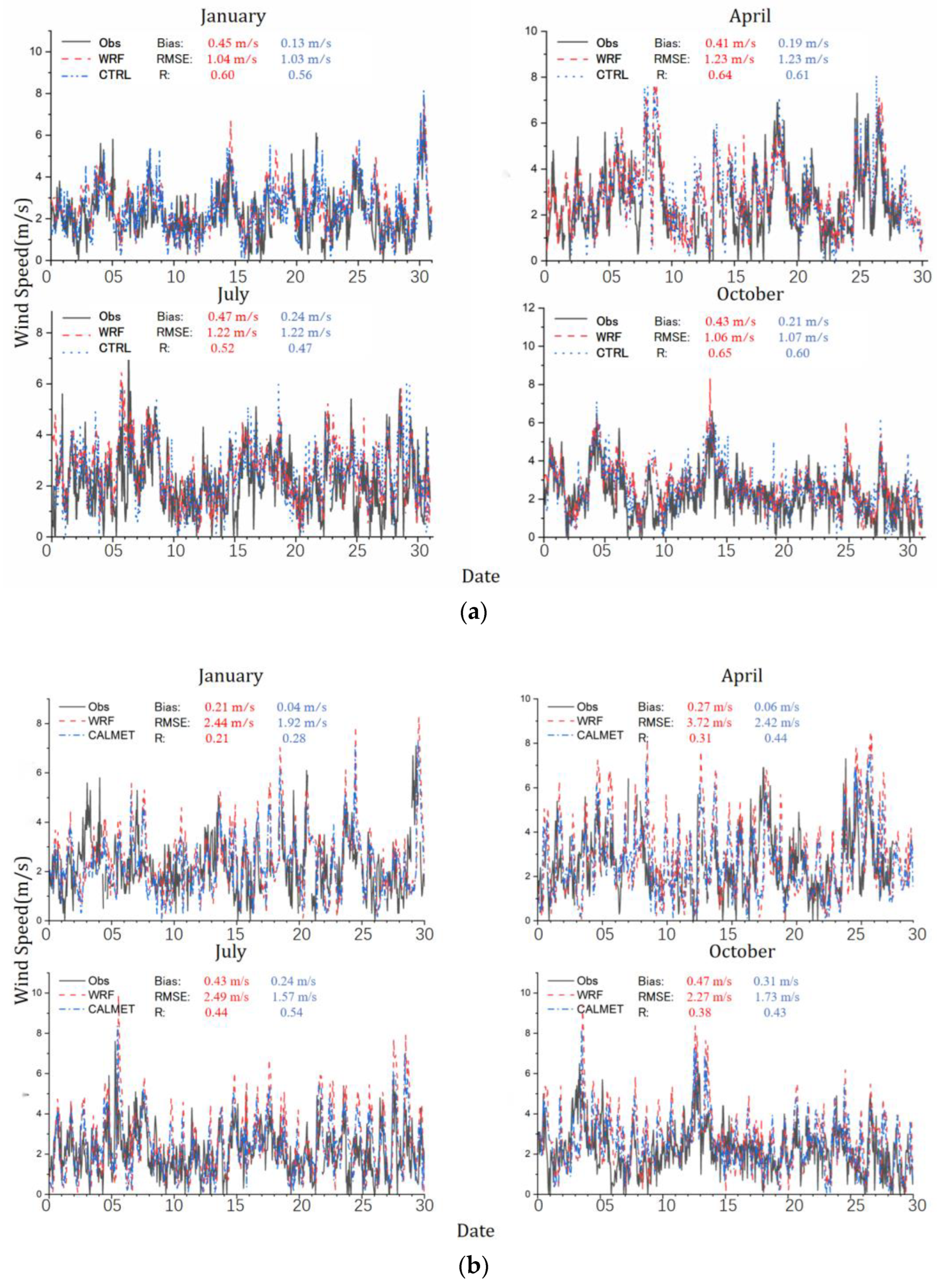
  • Improving the horizontal resolution of WRF to 300 m, updating the resolution of topographic elevation to ~100 m, and turning on the topographic wind correction can effectively improve the simulation results of wind direction, but there is no obvious improvement in wind speed.
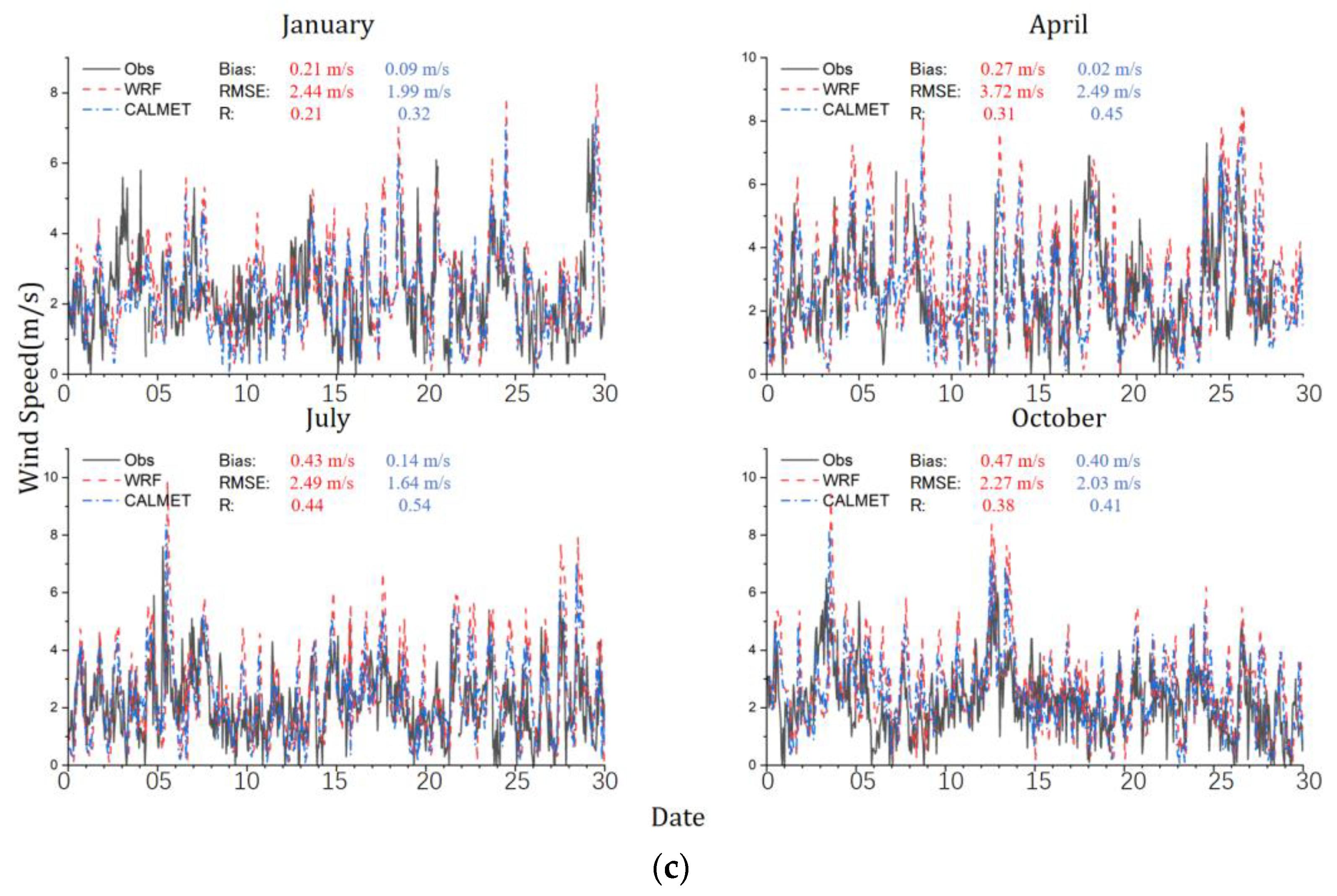
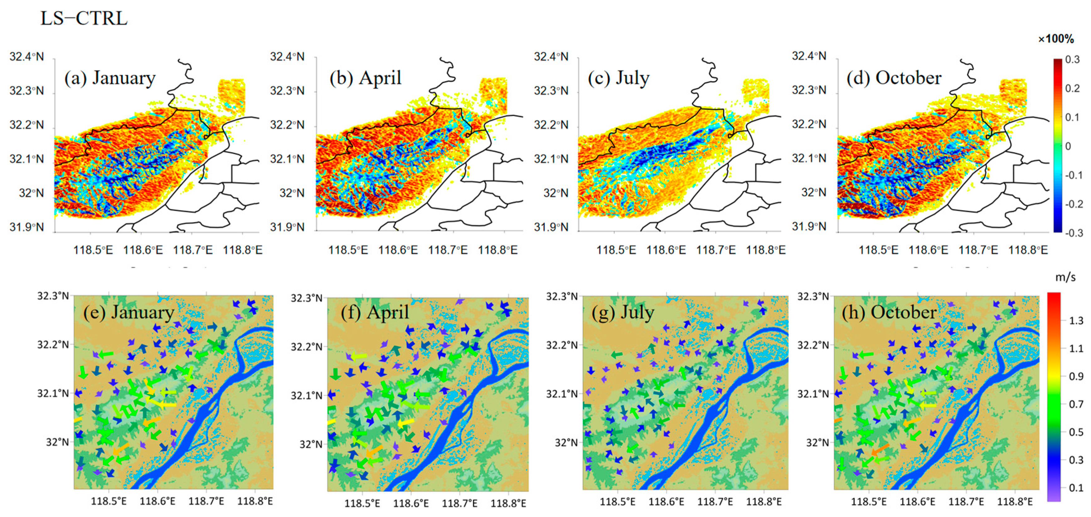
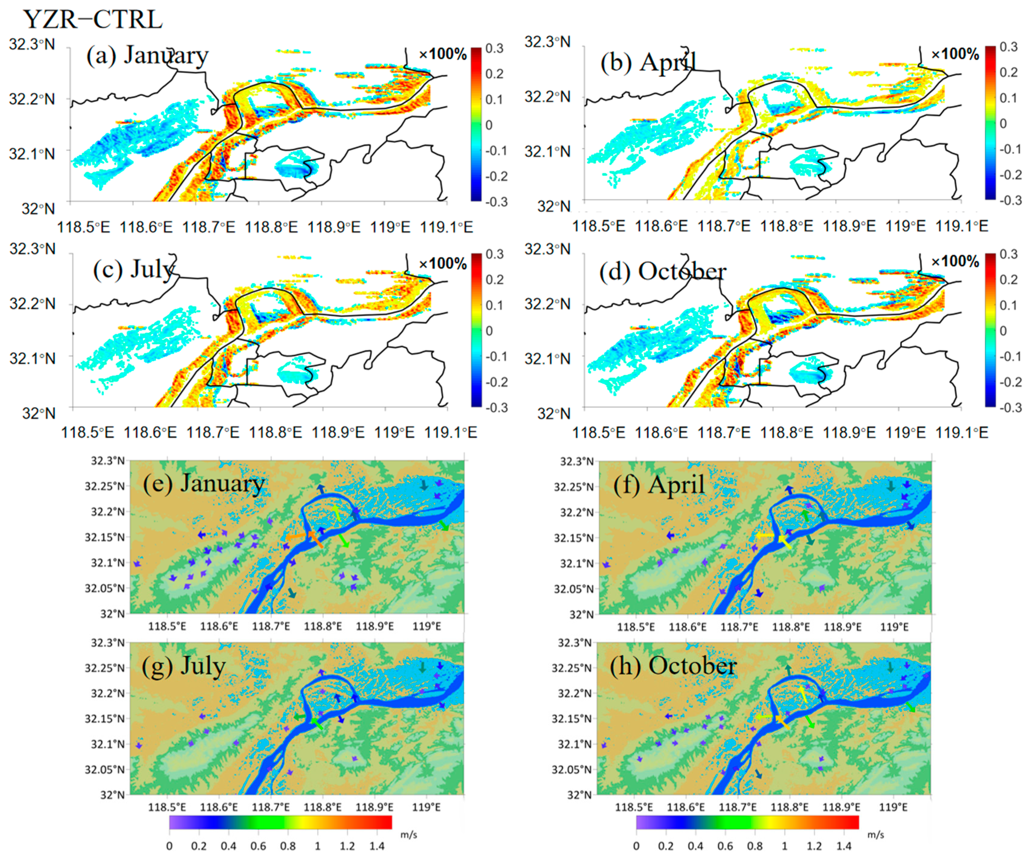
  • CALMET can further improve the simulation results of wind speed and direction. After updating the land cover types, the wind speed and direction improve more obviously under complex topographies. Mt. LS mainly blocks the upslope wind, and the ridge wind is weakened after “removing” Mt. LS. The Yangtze River mainly blocks the transport of PM2.5 from urban areas to the northwest of the river. After “removing” the Yangtze River, the transport channel from the south to the north of the river is more obvious at the south of Baguazhou where the Yangtze River splits.
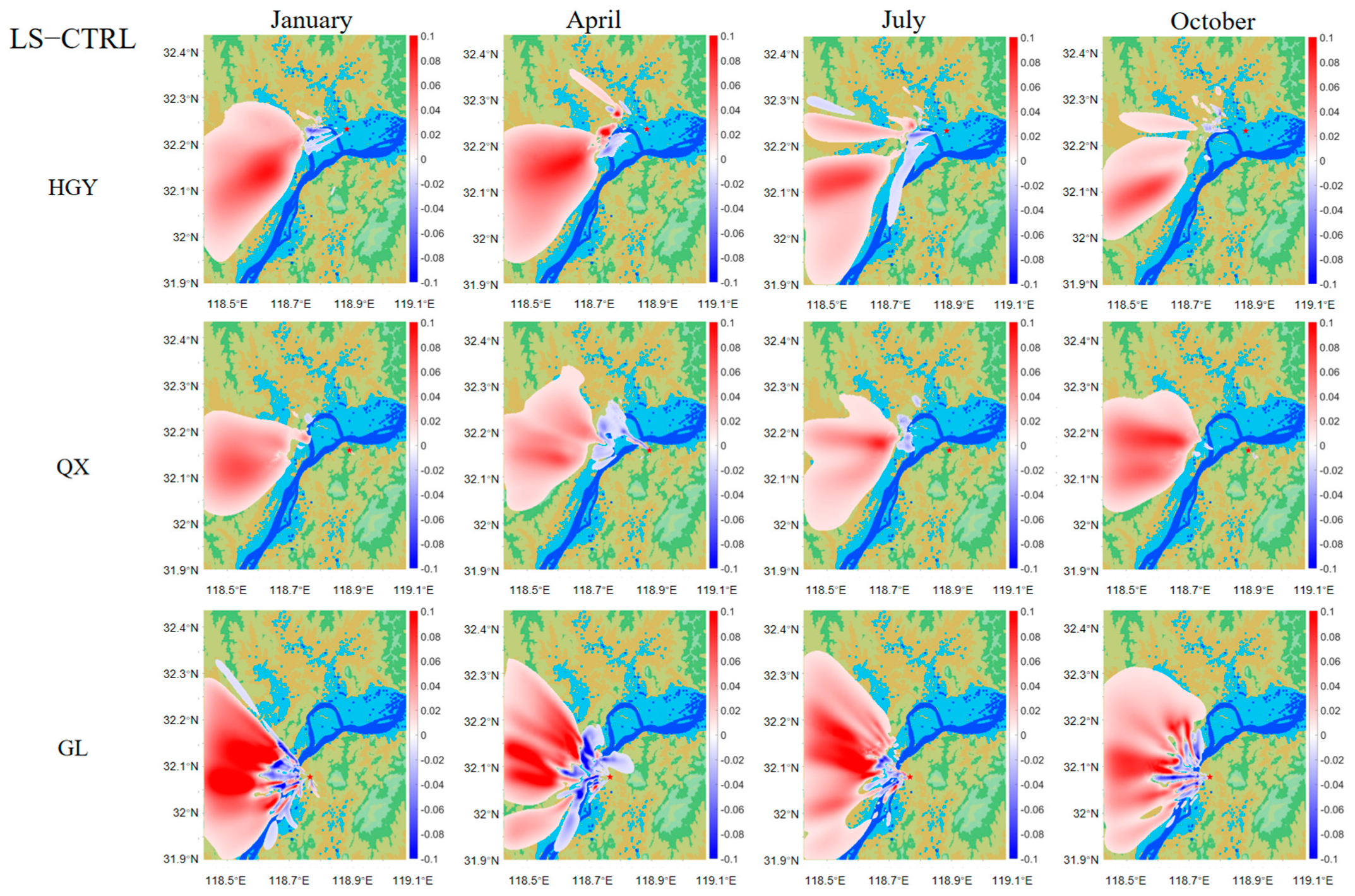
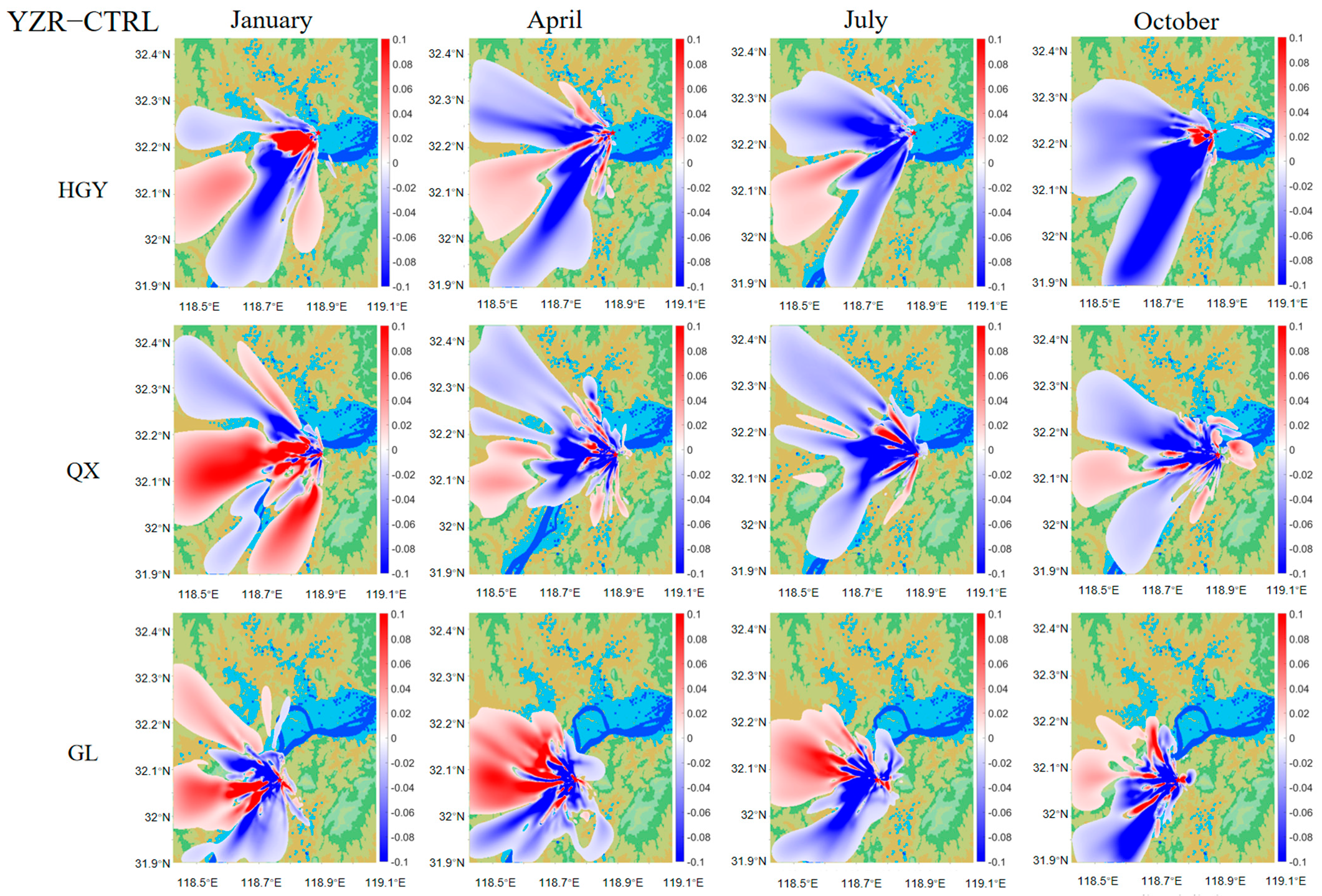
  • According to the simulation results of PM2.5 transport of virtual point sources, Mt. LS acts as a barrier, blocking PM2.5 diffusion and forcing PM2.5 transport to the south or southeast, and its influence on atmospheric PM2.5 level caused by PM2.5 emitted from Gulou District can reach 55%. The influence of the Yangtze River on PM2.5 transport is relatively divergent and has no obvious characteristics.
This study shows that the complex topographies have an obvious effect on the local wind field and the transport of atmospheric PM2.5. In the process of simulating local PM2.5, it is important to consider the influence of local topographies and land cover types on wind field. In addition, the observation of wind at meteorological Station PK basically reflects the influence of Mt. LS on the local wind field, but it is quite different from the dominant wind direction in Nanjing.

Supplementary Materials

The following supporting information can be downloaded at: https://www.mdpi.com/article/10.3390/atmos14050761/s1, Text S1: The impacts of Mt. LS and the Yangtze River on PM2.5 transport; Text S2: Comparisons of simulated and observed wind direction from different experiments; Text S3: The PM2.5 concentration and wind differences between WRF1000_CALMET1000 and WRF300_CALMET150_LU from experiments with three different virtual emission point sources; Text S4: comparisons of simulated and observed wind from different experiments at Liuhe Station; Figure S1: Spatial distributions of PM2.5 concentrations and the differences between before and after Mt. LS is “removed” from experiments with different point sources (ug/m3); Figure S2: Similar to Figure S1, but for the “removal” of the Yangtze River; Figure S3: Comparisons of simulated and observed wind direction from different experiments: WRF1000_CALMET150; WRF300_CALMET150; WRF300_CALMET150_LU; Figure S4: The PM2.5 concentration and wind differences between WRF1000_CALMET1000 and WRF300_CALMET150_LU from experiments with three different virtual emission point sources (ug/m3): Gulou District; Jiangbei Chemical Industry Park; Qixia District; Table S1: Verified wind speed of Liuhe Station; Table S2: Verified wind direction of Liuhe Station; Table S3: The symbols and units used in this manuscript.

Author Contributions

Conceptualization, Y.S. and M.S.; methodology, Y.S.; software, M.S.; validation, Y.S. and M.S.; formal analysis, M.S.; investigation, Y.S.; resources, M.S.; data curation, Y.S.; writing—original draft preparation, Y.S.; writing—review and editing, Y.S.; visualization, M.S.; supervision, M.S.; project administration, Y.S.; funding acquisition, M.S. All authors have read and agreed to the published version of the manuscript.

Funding

This work is funded by the Special Science and Technology Innovation Program for Carbon Peak and Carbon Neutralization of Jiangsu Province (Grant No. BE2022612).

Data Availability Statement

The meteorological observation data used in this study are the hourly observation data of wind speed and direction from the national meteorological stations PK and LH in Nanjing obtained from the China Meteorological Data Service Centre of the National Meteorological Information Centre (http://data.cma.cn/dataService/cdcindex/datacode/A.0012.0001/show_value/normal.html, access on 21 April 2023). The initial and boundary conditions for WRF simulation are provided by the Global Data Assimilation System (GDAS/FNL, DOI: 10.5065/D65Q4T4Z) with a horizontal resolution of 0.25° and a temporal resolution of 6 h.

Acknowledgments

We thank the UCAR group for providing the WRF model, we also thank Earth Tech, Inc. for providing the CALPUFF model.

Conflicts of Interest

The authors declare no conflict of interest.

References

  1. Mou, Y.; Song, Y.; Xu, Q.; He, Q.; Hu, A. Influence of urban-growth pattern on air quality in China: A study of 338 cities. Int. J. Environ. Res. Public Health. 2018, 15, 1805. [Google Scholar] [CrossRef]
  2. Zhan, D.; Kwan, M.P.; Zhang, W.; Yu, X.; Meng, B.; Liu, Q. The driving factors of air quality index in China. J. Clean. Prod. 2018, 197, 1342–1351. [Google Scholar] [CrossRef]
  3. Miao, Y.; Guo, J.; Liu, S.; Liu, H.; Li, Z.; Zhang, W.; Zhai, P. Classification of summertime synoptic patterns in Beijing and their associations with boundary layer structure affecting aerosol pollution. Atmos. Chem. Phys. 2017, 17, 3097–3110. [Google Scholar] [CrossRef]
  4. Wu, G.X.; Li, Z.Q.; Fu, C.B.; Zhang, X.Y.; Zhang, R.Y.; Zhang, R.H.; Zhou, T.J.; Li, J.P.; Li, J.D.; Zhou, D.G.; et al. Advances in studying interactions between aerosols and monsoon in China. Sci. China Earth Sci. 2016, 59, 1–16. [Google Scholar] [CrossRef]
  5. Zhang, J.P.; Zhu, T.; Zhang, Q.H.; Li, C.C.; Shu, H.L.; Ying, Y.; Dai, Z.P.; Wang, X.; Liu, X.Y.; Liang, A.M.; et al. The impact of circulation patterns on regional transport pathways and air quality over Beijing and its surroundings. Atmos. Chem. Phys. 2012, 12, 5031–5053. [Google Scholar] [CrossRef]
  6. Song, C.; Wu, L.; Xie, Y.; He, J.; Chen, X.; Wang, T.; Lin, Y.; Jin, T.; Wang, A.; Liu, Y.; et al. Air pollution in China: Status and spatiotemporal variations. Environ. Pollut. 2017, 227, 334–347. [Google Scholar] [CrossRef]
  7. He, J.; Gong, S.; Yu, Y.; Yu, L.; Wu, L.; Mao, H.; Song, C.; Zhao, S.; Liu, H.; Li, X.; et al. Air pollution characteristics and their relation to meteorological conditions during 2014–2015 in major Chinese cities. Environ. Pollut. 2017, 223, 484–496. [Google Scholar] [CrossRef] [PubMed]
  8. Liu, T.; Gong, S.; He, J.; Yu, M.; Wang, Q.; Li, H.; Liu, W.; Zhang, J.; Li, L.; Wang, X.; et al. Attributions of meteorological and emission factors to the 2015 winter severe haze pollution episodes in China’s Jing-Jin-Ji area. Atmos. Chem. Phys. 2017, 17, 2971–2980. [Google Scholar] [CrossRef]
  9. Quimbayo-Duarte, J.; Chemel, C.; Staquet, C.; Troude, F.; Arduini, G. Drivers of severe air pollution events in a deep valley during wintertime: A case study from the Arve river valley, France. Atmos. Environ. 2021, 247, 118030. [Google Scholar] [CrossRef]
  10. Jayaratne, R.; Pushpawela, B.; He, C.; Li, H.; Gao, J.; Chai, F.; Morawska, L. Observations of particles at their formation sizes in Beijing, China. Atmos. Chem. Phys. 2017, 17, 8825–8835. [Google Scholar] [CrossRef]
  11. Jacob, D.J.; Winner, D.A. Effect of climate change on air quality. Atmos. Environ. 2009, 43, 51–63. [Google Scholar] [CrossRef]
  12. Fu, G.Q.; Xu, W.Y.; Yang, R.F.; Li, J.B.; Zhao, C.S. The distribution and trends of fog and haze in the North China Plain over the past 30 years. Atmos. Chem. Phys. 2014, 14, 11949–11958. [Google Scholar] [CrossRef]
  13. Rigby, M.; Toumi, R. London air pollution climatology: Indirect evidence for urban boundary layer height and wind speed enhancement. Atmos. Environ. 2008, 42, 4932–4947. [Google Scholar] [CrossRef]
  14. Lehner, M.; Rotach, M. Current Challenges in Understanding and Predicting Transport and Exchange in the Atmosphere over Mountainous Terrain. Atmosphere 2018, 9, 276. [Google Scholar] [CrossRef]
  15. Jackson, P.L.; Mayr, G.; Vosper, S. Dynamically-driven winds. In Mountain Weather Research and Forecasting; Chow, T.K., Wekker, S.D., Snyder, B.J., Eds.; Springer: Berlin, Germany, 2013; Volume 3, pp. 121–218. [Google Scholar]
  16. Yu, Y.; Xu, H.; Jiang, Y.; Chen, F.; Cui, X.; He, J.; Liu, D. A modeling study of PM2.5 transboundary transport during a winter severe haze episode in southern Yangtze River Delta, China. Atmos. Res. 2021, 248, 105159. [Google Scholar] [CrossRef]
  17. Yang, J.; Tang, Y.; Han, S.; Liu, J.; Yang, X.; Hao, J. Evaluation and improvement study of the Planetary Boundary-Layer schemes during a high PM2. 5 episode in a core city of BTH region, China. Sci. Total Environ. 2021, 765, 142756. [Google Scholar] [CrossRef]
  18. Xie, B.; Fung, J.C.H.; Chan, A.; Lau, A. Evaluation of nonlocal and local planetary boundary layer schemes in the WRF model. J. Geophys. Res. Atmos. 2012, 117, D12103. [Google Scholar] [CrossRef]
  19. Zhang, Y.; Sartelet, K.; Zhu, S.; Wang, W.; Wu, S.Y.; Zhang, X.; Wang, K.; Tran, P.; Seigneur, C.; Wang, Z.F. Application of WRF/Chem-MADRID and WRF/Polyphemus in Europe—Part 2: Evaluation of chemical concentrations and sensitivity simulations. Atmos. Chem. Phys. 2013, 13, 6845–6875. [Google Scholar] [CrossRef]
  20. Yahya, K.; Zhang, Y.; Vukovich, J.M. Real-time air quality forecasting over the southeastern United States using WRF/Chem-MADRID: Multiple-year assessment and sensitivity studies. Atmos. Environ. 2014, 92, 318–338. [Google Scholar] [CrossRef]
  21. Cheng, W.Y.Y.; Steenburgh, W.J. Evaluation of Surface Sensible Weather Forecasts by the WRF and the Eta Models over the Western United States. Weather Forecast 2005, 20, 812–821. [Google Scholar] [CrossRef]
  22. Solazzo, E.; Bianconi, R.; Pirovano, G.; Moran, M.D.; Vautard, R.; Hogrefe, C.; Appel, K.W.; Matthias, V.; Grossi, P.; Bessagnet, B. Evaluating the capability of regional-scale air quality models to capture the vertical distribution of pollutants. Geosci. Model Dev. 2013, 6, 791–818. [Google Scholar] [CrossRef]
  23. Jiménez, P.A.; Dudhia, J. On the ability of the WRF model to reproduce the surface wind direction over complex terrain. J. Appl. Meteorol. Climatol. 2013, 52, 1610–1617. [Google Scholar] [CrossRef]
  24. Chow, F.K.; Weigel, A.P.; Street, R.L.; Rotach, M.W.; Xue, M. High-Resolution Large-Eddy Simulations of Flow in a Steep Alpine Valley. Part I: Methodology, Verification, and Sensitivity Experiments. J. Appl. Meteorol. Climatol. 2006, 45, 63–86. [Google Scholar] [CrossRef]
  25. Mirocha, J.D.; Kosovic, B.; Aitken, M.L.; Lundquist, J.K. Implementation of a generalized actuator disk wind turbine model into the weather research and forecasting model for large-eddy simulation applications. J. Renew. Sustain. Energy 2014, 6, 013104. [Google Scholar] [CrossRef]
  26. Shao, M.; Wang, Q.G.; Xu, J.J. Simulated Diurnal Cycles and Seasonal Variability of Low-level jets in the Boundary layer over Complex Terrain on the Coast of Southeast China. J. Geophys. Res. Atmos. 2017, 122, 10594–10611. [Google Scholar] [CrossRef]
  27. Skamarock, W.C.; Klemp, J.B.; Dudhia, J. A Description of the Advanced Research WRF Model Version 4.3 (No. NCAR/TN-556+STR). 2021. Available online: https://opensky.ucar.edu/islandora/object/technotes%3A588/datastream/PDF/view (accessed on 13 April 2023). [CrossRef]
  28. Yang, J.; Huang, X. The 30 m annual land cover dataset and its dynamics in China from 1990 to 2019. Earth Syst. Sci. Data 2021, 13, 3907–3925. [Google Scholar] [CrossRef]
  29. Mark, C.G.; Jin, X.; Narendra, A. Transport of Atmospheric Aerosol by Gap Winds in the Columbia River Gorge. J. Appl. Meteorol. Clim. 2008, 47, 15–26. [Google Scholar]
  30. Barman, N.; Gokhale, S. Urban black carbon-source apportionment, emissions and long-range transport over the Brahmaputra River Valley. Sci. Total Environ. 2019, 693, 133577. [Google Scholar] [CrossRef]
Figure 1. (a) Wind rose of LH Station from 2017 to 2019; (b) wind rose of PK Station from 2017 to 2019; (c) the simulation area of CALMET. The red dots are the locations of the LH and PK Stations, the red pentagrams are the locations of the virtual point sources, the mountainous areas are labeled with yellow text, and the shading is the topographic height (the dark blue area represents the Yangtze River).
Atmosphere 14 00761 g001
Figure 2. Comparisons of downscaled wind speed from different experiments: (a) WRF1000_CALMET150; (b) WRF300_CALMET150; (c) WRF300_CALMET150_LU.
Atmosphere 14 00761 g002aAtmosphere 14 00761 g002b
Figure 3. Differences in wind field between “removing” Mt. LS and CTRL: (ad) monthly mean wind speed differences; (eh) monthly mean wind vector differences (colored arrows).
Atmosphere 14 00761 g003
Figure 4. Similar to Figure 3, but for Yangtze River. The dark red circle in (a) is the south side of Baguazhou (an island in the Yangtze River) where the Yangtze River splits: (ad) monthly mean wind speed differences; (eh) monthly mean wind vector differences (colored arrows).
Atmosphere 14 00761 g004
Figure 5. Variations of the spatial distribution of monthly mean PM2.5 concentration simulated by CALPUFF after “removing” Mt. LS. First row: LS_HGY–CTRL_HGY; second row: LS_QX–CTRL_QX; third row: LS_GLCTRL_GL.
Atmosphere 14 00761 g005
Figure 6. Similar to Figure 5, but for the “removal” of Yangtze River.
Atmosphere 14 00761 g006
Table 1. Configurations of WRF.
The Settings of the Study Area
Experiment nameWRF1000WRF300
Initial condition GDAS/FNL 0.25° × 0.25° (DOI: 10.5065/D65Q4T4Z)
Projection/central geolocationLambert/(119° E, 33° N)
TopographyGMTED2010 (30s, ~1 km)/SRTM (~100 m)
Integration step60 s30 s
Three layers of nestingD01 (9 km), 229 × 279D01 (7.5 km), 92 × 94
D02 (3 km), 276 × 312D02 (1.5 km), 106 × 151
D03 (1000 m), 123 × 177D03 (300 m), 266 × 311
Vertical resolution37 layers from near ground to 100 hPa (4 layers between 1013 hPa and 1000 hPa)
Microphysical processNew Thompson et al. scheme
Radiation schemeRRTMG
Cumulus parameterization schemeNone
Near-surface layer schemeEta Similarity
Land surface processNoah Land Surface Model
Boundary layer + topography correctionYonsei University scheme + Topo_wind = 0Yonsei University scheme + Topo_wind = 1
Table 2. CALPUFF experiment setup.
Experiment NameSettings of Topographies and Virtual Point Sources
CTRL_HGYReal topographies, virtual point source in Jiangbei Chemical Industry Park
CTRL_QXReal topographies, virtual point source in Qixia District
CTRL_GLReal topographies, virtual point source in Gulou District
LS_HGY“Remove” LS, virtual point source in Jiangbei Chemical Industry Park
LS_QX“Remove” LS, virtual point source in Qixia District
LS_GL“Remove” LS, virtual point source in Gulou District
YZR_HGY“Remove” the Yangtze River and its coastal areas, virtual point source is in Jiangbei Chemical Industry Park
YZR_QX“Remove” the Yangtze River and its coastal areas, virtual point source in Qixia District
YZR_GL“Remove” the Yangtze River and its coastal areas, virtual point source in Gulou District
Table 3. Statistics of wind direction evaluation.
MonthIndexWRF1000_CALMET150WRF300_CALMET150WRF300_CALMET150_LU
WRFCALMETWRFCALMETWRFCALMET
JanuaryAbias100.4°95.5°53.3°51.8°53.3°46.6°
RMSE140.5°135.5°70.9°69.7°70.9°63.2°
AprilAbias75.3°72.6°48.3°47.2°48.3°41.0°
RMSE102.9°102.7°64.3°62.5°64.3°56.5°
JulyAbias90.1°90.4°55.3°60.3°55.3°54.4°
RMSE127.9°130.2°71.6°77.6°71.6°70.2°
OctoberAbias112.6°119.6°44.4°48.3°44.5°40.5°
RMSE162.1°166.6°59.6°64.1°59.6°56.0°
Table 4. Monthly domain averaged percentage variation of PM2.5 concentration by “removing” Mt. LS (%).
Point SourceMean Concentration
Variation
JanuaryAprilJulyOctober
HGYAverage increase24.2 21.4 22.0 22.5
HGYAverage decrease−11.8 −11.5 −13.8 −13.9
QXAverage increase25.4 23.1 18.3 31.1
QXAverage decrease−10.1 −14.9 −14.5 −10.7
GLAverage increase55.0 47.4 40.0 32.7
GLAverage decrease−25.2 −33.7 −27.0 −31.7
Disclaimer/Publisher’s Note: The statements, opinions and data contained in all publications are solely those of the individual author(s) and contributor(s) and not of MDPI and/or the editor(s). MDPI and/or the editor(s) disclaim responsibility for any injury to people or property resulting from any ideas, methods, instructions or products referred to in the content.

