

Short-Term Probabilistic Forecasting Method for Wind Speed Combining Long Short-Term Memory and Gaussian Mixture Model

Abstract
:1. Introduction
2. Methodology
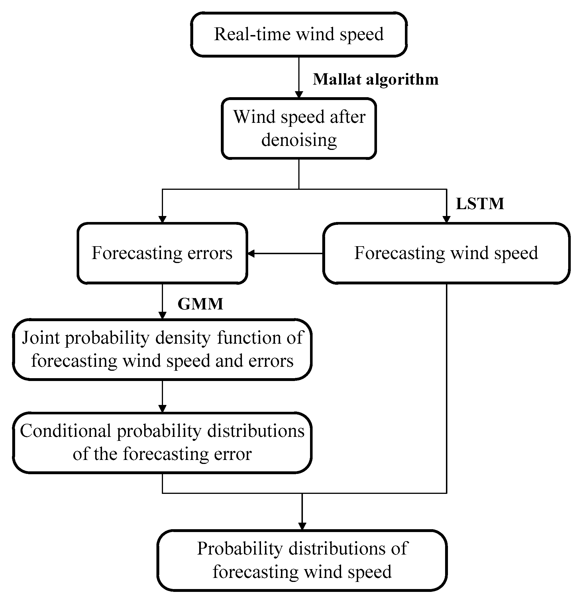
2.1. Flowchart of Methodology
- (1)
- The wind speed in the current step, , is assumed to be the real-time monitored data obtained by an anemometer. The data are filtered in real time using the Mallat algorithm [39] to reduce the influence of the high-frequency component on the precision of wind speed prediction.
- (2)
- The wind speed in the next step, , is then predicted using the LSTM method from the denoised sequence of the previous wind speed. The forecast wind speed, , is treated as the mean value of the probabilistically predicted wind speed in the next step.
- (3)
- The errors of the previously predicted wind speed, , are calculated by comparing the measured wind speed, , and forecast speed, .
- (4)
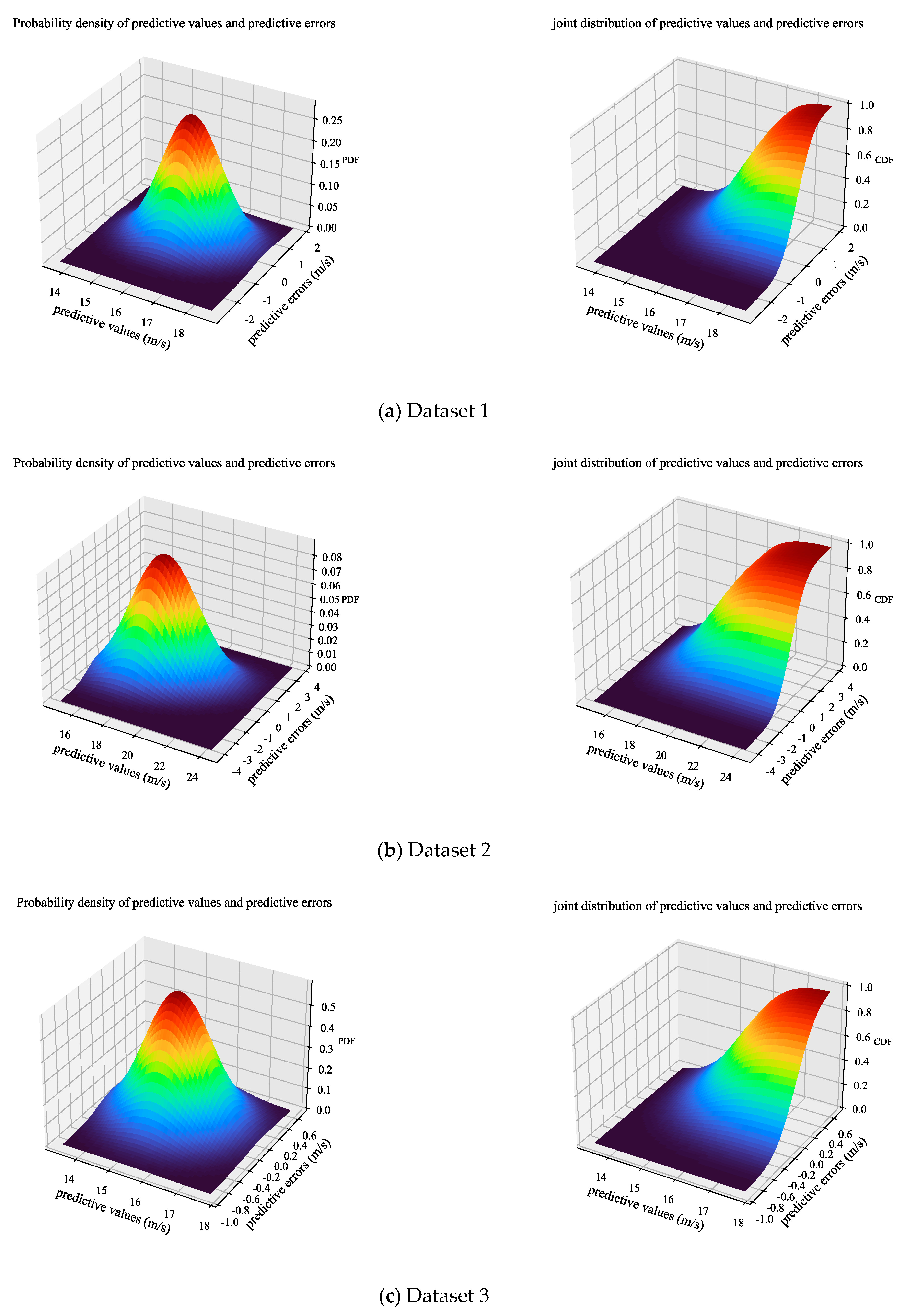
- The key parameters of the joint PDF of the predicted wind speeds and errors are identified using the GMM method.
- (5)
- The conditional probability distributions and corresponding covariance of the prediction errors of the forecast wind speed, , are calculated.
- (6)
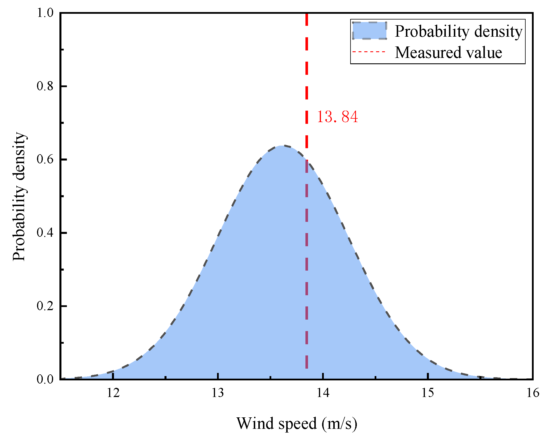
- The forecast wind speed, , is the mean, and the covariance of error, , is the covariance of . The probability distributions of the predicted wind speed follow the normal distribution, .
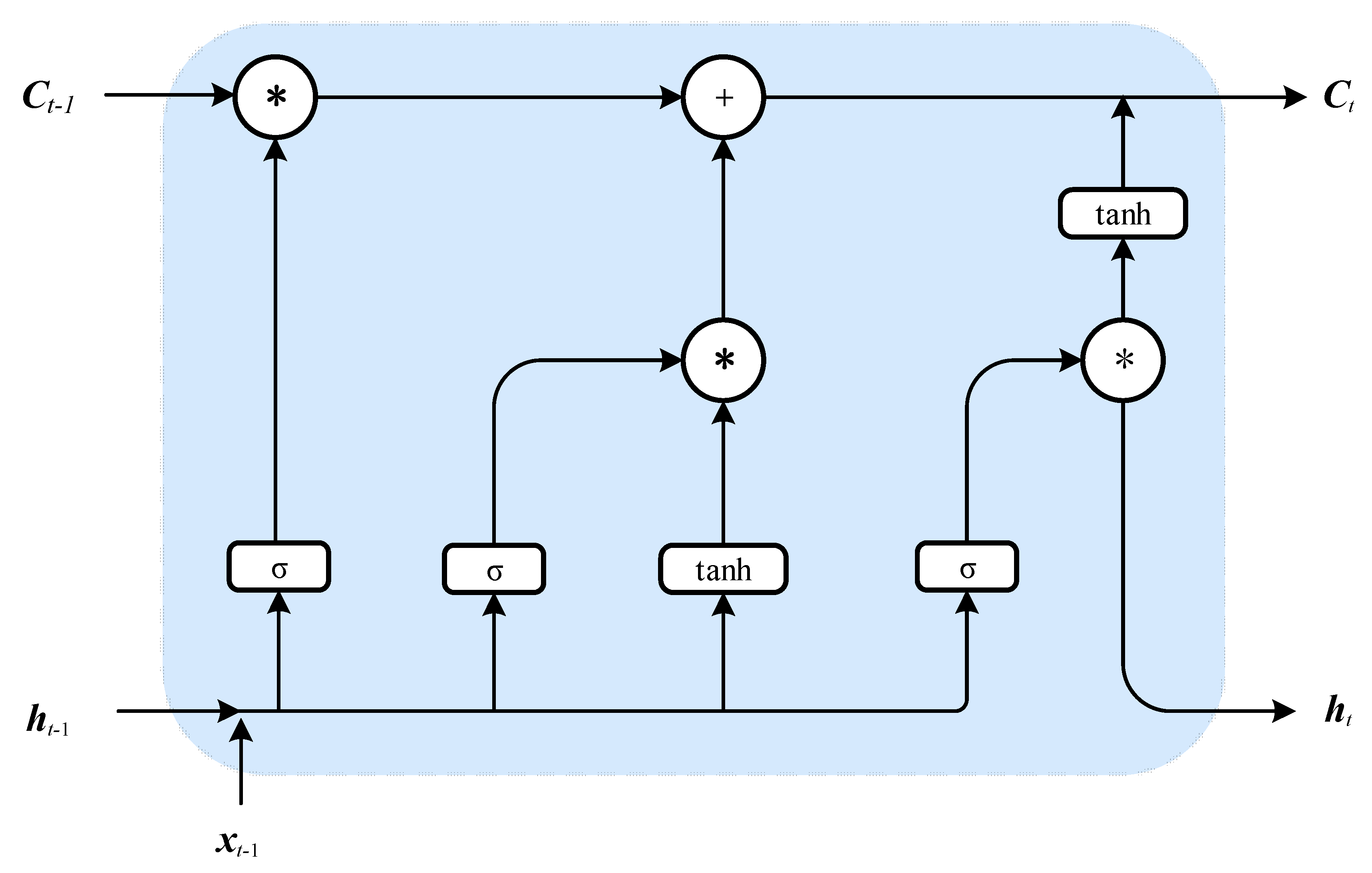
2.2. LSTM Method
- To avoid overfitting, the number of LSTM network layers must not be overly high [25]. Accordingly, in the present study, the network only consists of two LSTM layers: a dropout and two fully connected layers.
- The maximum number of epochs is set to 50.
- In the training process, the batch size for updating the weights of the LSTM network was set to 128.
- An Adam optimizer [43] with a learning rate of 10−4 is used.
2.3. GMM Method
2.4. Conditional PDF of Forecasting Errors
2.5. Indicators of Prediction Precision
3. Validation
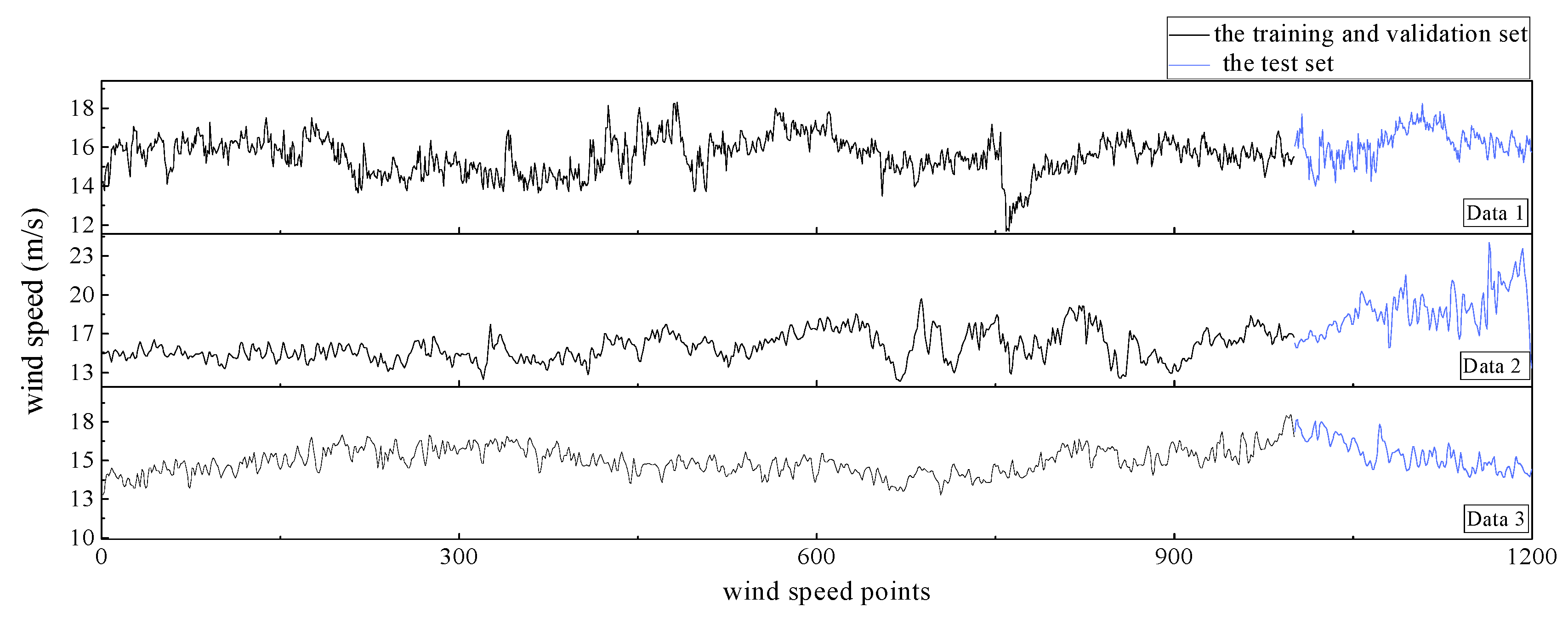
3.1. Data Sources and Processing
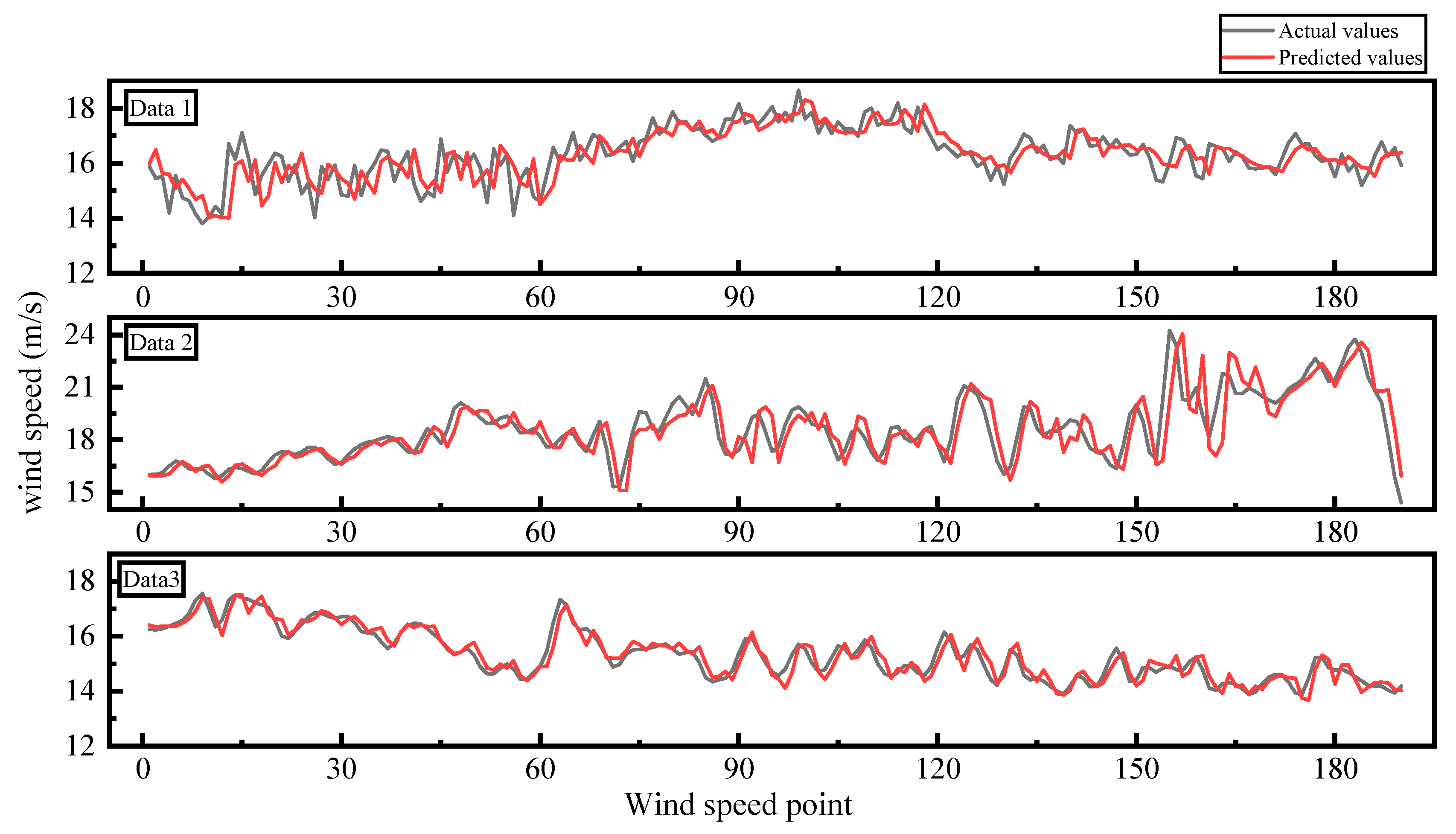
3.2. Forecasting Wind Speed by LSTM
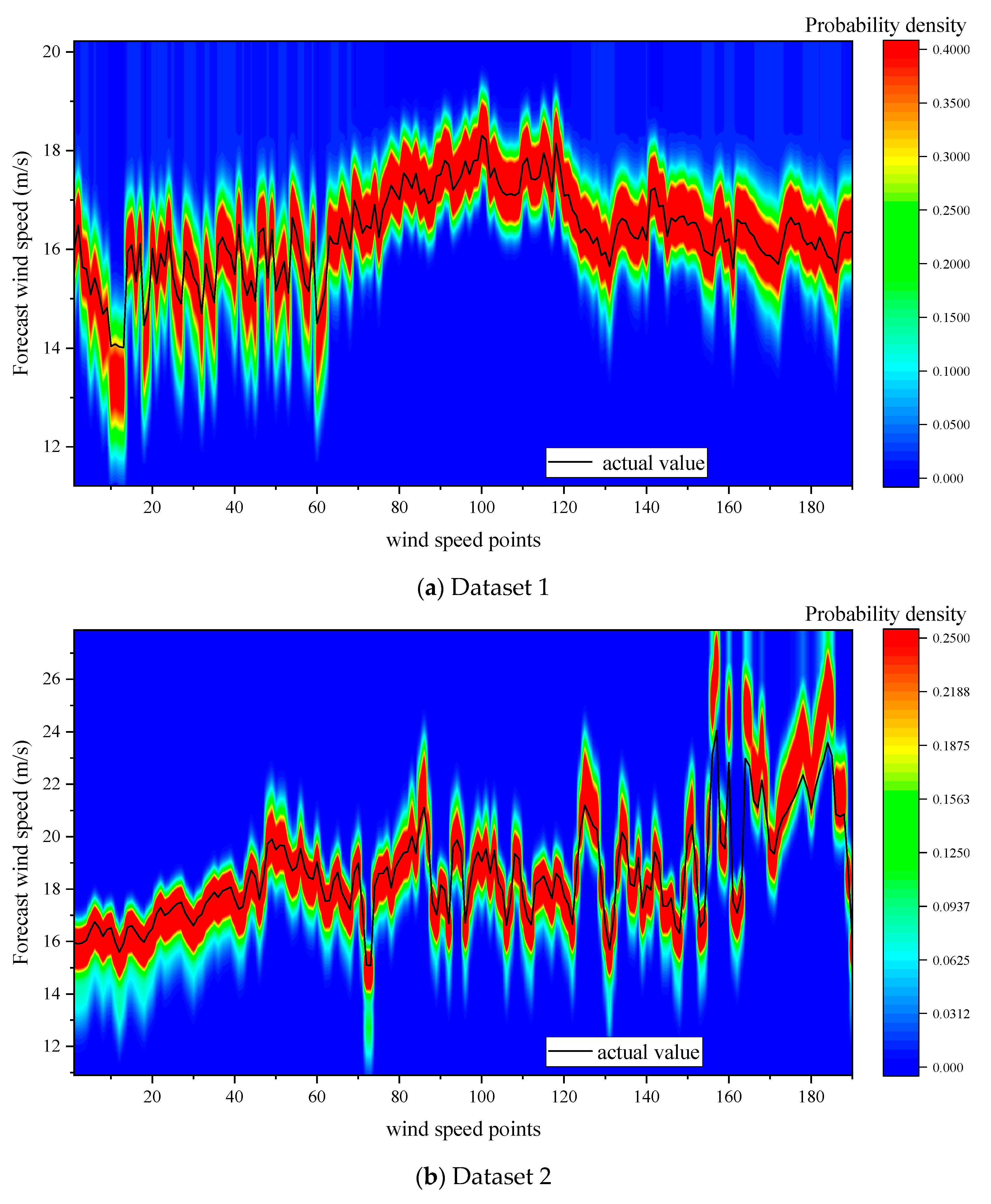
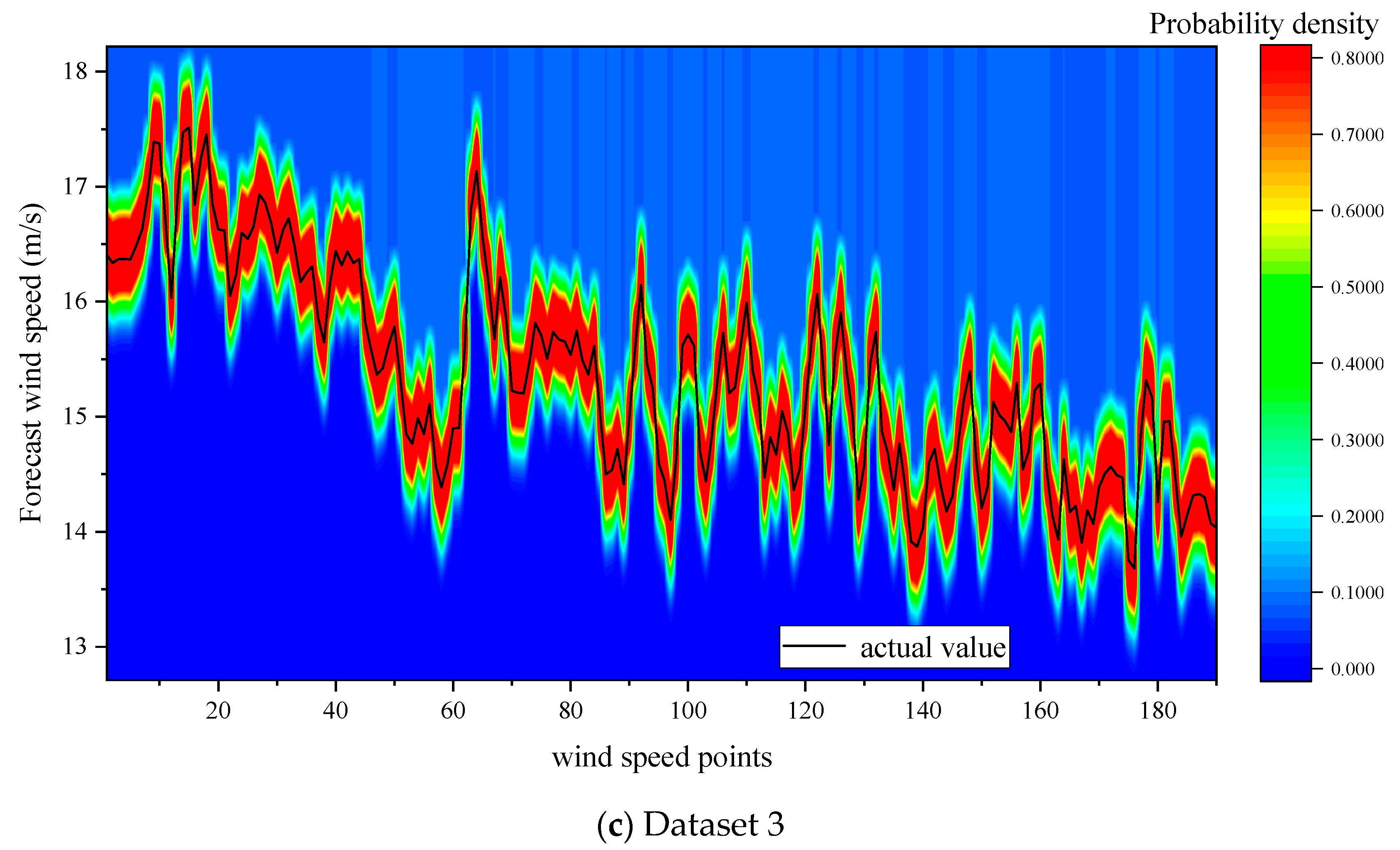
3.3. GMM Fitting and Probabilistic Forecasting Results
4. Precision Analysis
4.1. Precision Indicators
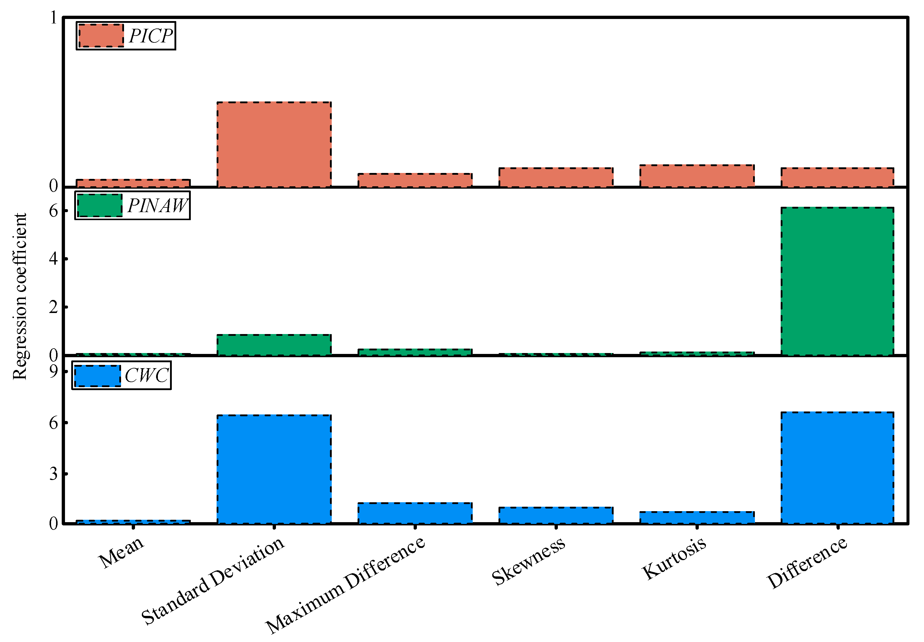
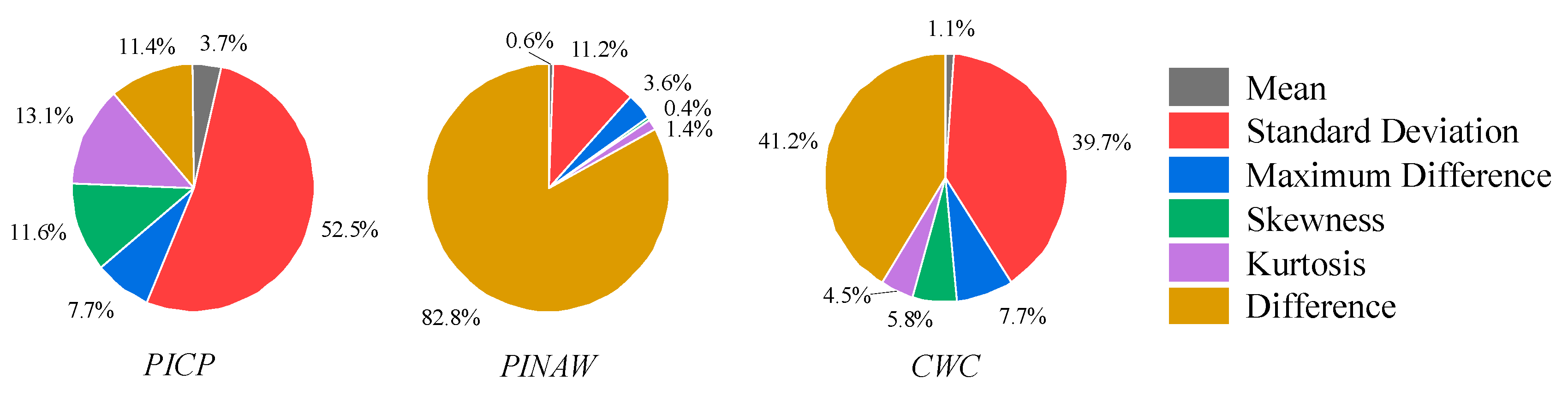
4.2. Effects of Wind Speed Characteristic on Precision
5. Conclusions
Author Contributions
Funding
Institutional Review Board Statement
Informed Consent Statement
Data Availability Statement
Conflicts of Interest
References
- Hui, L.; Tian, H.Q.; Chen, C.; Li, Y.F. A hybrid statistical method to predict wind speed and wind power. Renew. Energy 2010, 35, 1857–1861. [Google Scholar]
- Hui, L.; Hong-Qi, T.; Yan-Fei, L.I. Short-term forecasting optimization algorithms for wind speed along Qinghai-Tibet railway based on different intelligent modeling theories. J. Cent. South Univ. Technol. 2009, 16, 690–696. [Google Scholar]
- Noboru, K. Toward a New Stage of Mori Ogai Studies. Teikoku Gakushiin Kiji 2007, 58, 61–96. [Google Scholar]
- Jie, Y.; Liu, Y.; Shuang, H.; Wang, Y.; Feng, S. Reviews on uncertainty analysis of wind power forecasting. Renew. Sustain. Energy Rev. 2015, 52, 1322–1330. [Google Scholar]
- Cheng, W.Y.Y.; Liu, Y.; Bourgeois, A.J.; Wu, Y.; Haupt, S.E. Short-term wind forecast of a data assimilation/weather forecasting system with wind turbine anemometer measurement assimilation. Renew. Energy 2017, 107, 340–351. [Google Scholar] [CrossRef]
- Yang, J.; Astitha, M.; Monache, L.D.; Alessandrini, S. An Analog Technique to Improve Storm Wind Speed Prediction Using a Dual NWP Model Approach. Mon. Weather. Rev. 2018, 146, 4057–4077. [Google Scholar] [CrossRef]
- Wang, H.; Han, S.; Liu, Y.; Yan, J.; Li, L. Sequence transfer correction algorithm for numerical weather prediction wind speed and its application in a wind power forecasting system. Appl. Energy 2019, 237, 1–10. [Google Scholar] [CrossRef]
- Pearre, N.S.; Swan, L.G. Statistical approach for improved wind speed forecasting for wind power production. Sustain. Energy Technol. Assessments 2018, 27, 180–191. [Google Scholar] [CrossRef]
- Do, D.-P.N.; Lee, Y.; Choi, J. Hourly Average Wind Speed Simulation and Forecast Based on ARMA Model in Jeju Island, Korea. J. Electr. Eng. Technol. 2016, 11, 1548–1555. [Google Scholar] [CrossRef] [Green Version]
- Yunus, K.; Thiringer, T.; Chen, P. ARIMA-Based Frequency-Decomposed Modeling of Wind Speed Time Series. IEEE Trans. Power Syst. 2015, 31, 2546–2556. [Google Scholar] [CrossRef]
- Yan, L.; Wang, H.; Zhang, X.; Li, M.Y.; He, J. Impact of meteorological factors on the incidence of bacillary dysentery in Beijing, China: A time series analysis (1970–2012). PLoS ONE 2017, 12, e0182937. [Google Scholar] [CrossRef] [PubMed] [Green Version]
- Li, P.; Wang, Y.; Dong, Q. The analysis and application of a new hybrid pollutants forecasting model using modified Kolmogorov-Zurbenko filter. Sci. Total Environ. 2017, 583, 228–240. [Google Scholar] [CrossRef] [PubMed]
- Huang, Z.; Gu, M. Characterizing Nonstationary Wind Speed Using the ARMA-GARCH Model. J. Struct. Eng. 2019, 145, 04018226. [Google Scholar] [CrossRef]
- Ouarda, T.B.; Charron, C. Non-stationary statistical modelling of wind speed: A case study in eastern Canada. Energy Convers. Manag. 2021, 236, 114028. [Google Scholar] [CrossRef]
- Jeong, J.; Lee, S.-J. A Statistical Parameter Correction Technique for WRF Medium-Range Prediction of Near-Surface Temperature and Wind Speed Using Generalized Linear Model. Atmosphere 2018, 9, 291. [Google Scholar] [CrossRef] [Green Version]
- Galanis, G.; Papageorgiou, E.; Liakatas, A. A hybrid Bayesian Kalman filter and applications to numerical wind speed modeling. J. Wind. Eng. Ind. Aerodyn. 2017, 167, 1–22. [Google Scholar] [CrossRef]
- Tian, Z. Short-term wind speed prediction based on LMD and improved FA optimized combined kernel function LSSVM. Eng. Appl. Artif. Intell. 2020, 91, 103573. [Google Scholar] [CrossRef]
- Wang, J.; Yang, Z. Ultra-short-term wind speed forecasting using an optimized artificial intelligence algorithm. Renew. Energy 2021, 171, 1–5. [Google Scholar] [CrossRef]
- Liu, H.; Tian, H.-Q.; Li, Y.-F. Comparison of two new ARIMA-ANN and ARIMA-Kalman hybrid methods for wind speed prediction. Appl. Energy 2012, 98, 415–424. [Google Scholar] [CrossRef]
- Hu, Y.-L.; Chen, L. A nonlinear hybrid wind speed forecasting model using LSTM network, hysteretic ELM and Differential Evolution algorithm. Energy Convers. Manag. 2018, 173, 123–142. [Google Scholar] [CrossRef]
- Gangwar, S.; Bali, V.; Kumar, A. Comparative Analysis of Wind Speed Forecasting Using LSTM and SVM. ICST Trans. Scalable Inf. Syst. 2018, 7, 159407. [Google Scholar] [CrossRef]
- Kumar, V.; Pal, Y.; Tripathi, M.M. SVM Tuned NARX Method for Wind speed & power Prediction in Electricity Generation. In Proceedings of the 8th IEEE Power India International Conference (PIICON), Kurukshetra, India, 10–12 December 2018. [Google Scholar]
- Liu, H.; Mi, X.; Li, Y. Smart multi-step deep learning model for wind speed forecasting based on variational mode decomposition, singular spectrum analysis, LSTM network and ELM. Energy Convers. Manag. 2018, 159, 54–64. [Google Scholar] [CrossRef]
- Huai, N.N.; Dong, L.; Wang, L.J.; Ying, H.; Zhongjian, D.; Bo, W. Short-term Wind Speed Prediction Based on CNN_GRU Model. In Proceedings of the 31st Chinese Control And Decision Conference (CCDC), Nanchang, China, 3–5 June 2019; pp. 2243–2247. [Google Scholar]
- Feng, C.; Cui, M.; Hodge, B.-M.; Zhang, J. A data-driven multi-model methodology with deep feature selection for short-term wind forecasting. Appl. Energy 2017, 190, 1245–1257. [Google Scholar] [CrossRef] [Green Version]
- Wang, H.-Z.; Li, G.-Q.; Wang, G.-B.; Peng, J.-C.; Jiang, H.; Liu, Y.-T. Deep learning based ensemble approach for probabilistic wind power forecasting. Appl. Energy 2017, 188, 56–70. [Google Scholar] [CrossRef]
- Zhang, W.; Qu, Z.; Zhang, K.; Mao, W.; Ma, Y.; Fan, X. A combined model based on CEEMDAN and modified flower pollination algorithm for wind speed forecasting. Energy Convers. Manag. 2017, 136, 439–451. [Google Scholar] [CrossRef]
- Zhang, Y.; Chen, B.; Pan, G.; Zhao, Y. A novel hybrid model based on VMD-WT and PCA-BP-RBF neural network for short-term wind speed forecasting. Energy Convers. Manag. 2019, 195, 180–197. [Google Scholar] [CrossRef]
- Liu, Z.; Hara, R.; Kita, H. 24 h-ahead wind speed forecasting using CEEMD-PE and ACO-GA-based deep learning neural network. J. Renew. Sustain. Energy 2021, 13, 046101. [Google Scholar] [CrossRef]
- Bahrami, S.; Hooshmand, R.A.; Parastegari, M. Short term electric load forecasting by wavelet transform and grey model improved by PSO (particle swarm optimization) algorithm—ScienceDirect. Energy 2014, 72, 434–442. [Google Scholar] [CrossRef]
- Li, Y.; Wu, H.; Liu, H. Multi-step wind speed forecasting using EWT decomposition, LSTM principal computing, RELM subordinate computing and IEWT reconstruction. Energy Convers. Manag. 2018, 167, 203–219. [Google Scholar] [CrossRef]
- Wang, J.; Niu, T.; Lu, H.; Yang, W.; Du, P. A Novel Framework of Reservoir Computing for Deterministic and Probabilistic Wind Power Forecasting. IEEE Trans. Sustain. Energy 2019, 1, 1. [Google Scholar] [CrossRef]
- Dan, L.; Fja, B.; Min, C.; Qian, T. Multi-step-ahead wind speed forecasting based on a hybrid decomposition method and temporal convolutional networks. Energy 2021, 238, 121981. [Google Scholar]
- Yousuf, M.U.; Al-Bahadly, I.; Avci, E. Current Perspective on the Accuracy of Deterministic Wind Speed and Power Forecasting. IEEE Access 2019, 7, 159547–159564. [Google Scholar] [CrossRef]
- Yin, J.; Tang, T.; Yang, L.; Xun, J.; Huang, Y.; Gao, Z. Research and development of automatic train operation for railway transportation systems: A survey. Transp. Res. Part C Emerg. Technol. 2017, 85, 548–572. [Google Scholar] [CrossRef]
- Liu, Y.; Qin, H.; Zhang, Z.; Pei, S.; Jiang, Z.; Feng, Z.; Zhou, J. Probabilistic spatiotemporal wind speed forecasting based on a variational Bayesian deep learning model. Appl. Energy 2020, 260, 114259. [Google Scholar] [CrossRef]
- Najibi, F.; Apostolopoulou, D.; Alonso, E. Enhanced performance Gaussian process regression for probabilistic short-term solar output forecast. Int. J. Electr. Power Energy Syst. 2021, 130, 106916. [Google Scholar] [CrossRef]
- Hernandez, H. Multivariate probability theory: Determination of probability density functions. Res. Rep. 2017. [Google Scholar] [CrossRef]
- Mallat, S.G. A theory for multiresolution signal decomposition: The wavelet representation. IEEE Trans. Pattern Anal. Mach. Intell. 1989, 11, 674–693. [Google Scholar] [CrossRef] [Green Version]
- Hochreiter, S.; Schmidhuber, J. Long short-term memory. Neural Comput. 1997, 9, 1735–1780. [Google Scholar] [CrossRef]
- Liu, Y.; Guan, L.; Hou, C.; Han, H.; Liu, Z.; Sun, Y.; Zheng, M. Wind Power Short-Term Prediction Based on LSTM and Discrete Wavelet Transform. Appl. Sci. 2019, 9, 1108. [Google Scholar] [CrossRef] [Green Version]
- Greff, K.; Srivastava, R.K.; Koutník, J.; Steunebrink, B.R.; Schmidhuber, J. LSTM: A search space odyssey. IEEE Trans. Neural Netw. Learn. Syst. 2016, 28, 2222–2232. [Google Scholar] [CrossRef] [Green Version]
- Kingma, D.; Ba, J. Adam: A Method for Stochastic Optimization. arXiv 2014, arXiv:1412.6980. [Google Scholar]
- Xu, L.; Jordan, M.I. On convergence properties of the EM algorithm for Gaussian mixtures. Neural Comput. 1996, 8, 129–151. [Google Scholar] [CrossRef]
- Dempster, P.; Laird, N.M.; Rubin, D.B. Maximum likelihood from incomplete data via the EM algorithm (With discussion). Jroystatistsocserb 1977, 39, 1–22. [Google Scholar]
- Wu, W.; Qiao, Y.; Lu, Z.; Wang, N.; Zhou, Q. Methods and prospects for probabilistic forecasting of wind power. Autom. Electr. Power Syst. 2017, 41, 167–175. [Google Scholar]
- Khosravi, A.; Nahavandi, S.; Creighton, D. Prediction Intervals for Short-Term Wind Farm Power Generation Forecasts. IEEE Trans. Sustain. Energy 2013, 4, 602–610. [Google Scholar] [CrossRef]
- Frantál, B.; Nováková, E. On the spatial differentiation of energy transitions: Exploring determinants of uneven wind energy developments in the Czech Republic. Morav. Geogr. Rep. 2019, 27, 79–91. [Google Scholar] [CrossRef] [Green Version]


| Dataset No. | Mean (m/s) | Standard Deviation (m/s) | Maximum Difference (m/s) | Skewness (m3/s3) | Kurtosis (m4/s4) | Difference (m/s) |
|---|---|---|---|---|---|---|
| 1 | 15.72 | 7.59 | 1.11 | −0.33 | 3.47 | 0.48 |
| 2 | 16.67 | 5.95 | 1.22 | −0.19 | 2.30 | 0.28 |
| 3 | 17.28 | 5.60 | 1.03 | 0.05 | 2.48 | 0.30 |
| 4 | 17.20 | 7.94 | 1.31 | −1.41 | 5.31 | 0.36 |
| 5 | 16.96 | 4.34 | 0.75 | 0.07 | 2.72 | 0.22 |
| 6 | 15.89 | 11.84 | 1.77 | 1.16 | 4.93 | 0.35 |
| 7 | 16.74 | 3.17 | 0.58 | −0.05 | 2.70 | 0.21 |
| 8 | 15.03 | 5.20 | 0.89 | 0.32 | 2.99 | 0.23 |
| 9 | 15.81 | 3.36 | 0.53 | −0.1 | 2.90 | 0.27 |
| 10 | 15.69 | 4.79 | 0.95 | 0.19 | 2.08 | 0.19 |
| 11 | 15.08 | 7.74 | 1.60 | 0.05 | 2.27 | 0.24 |
| 12 | 16.00 | 5.15 | 0.81 | 0.23 | 3.70 | 0.24 |
| 13 | 15.41 | 7.40 | 1.25 | 0.36 | 3.05 | 0.28 |
| 14 | 15.24 | 7.43 | 1.18 | −1.48 | 6.24 | 0.19 |
| 15 | 11.64 | 9.59 | 1.53 | −0.76 | 4.47 | 0.29 |
| 16 | 12.23 | 11.32 | 2.01 | −0.74 | 3.57 | 0.64 |
| 17 | 10.21 | 11.96 | 2.24 | 0.80 | 3.58 | 0.36 |
| 18 | 8.77 | 5.12 | 0.94 | 0.12 | 2.77 | 0.18 |
| 19 | 8.33 | 8.70 | 1.53 | 0.52 | 3.10 | 0.23 |
| 20 | 13.00 | 3.57 | 0.88 | 0.08 | 1.75 | 0.10 |
| 21 | 11.46 | 3.01 | 0.46 | −0.47 | 3.34 | 0.09 |
| 22 | 11.00 | 4.82 | 0.93 | 0.90 | 3.52 | 0.13 |
| 23 | 7.82 | 6.10 | 1.16 | 0.67 | 2.98 | 0.23 |
| 24 | 7.51 | 4.40 | 0.75 | 0.67 | 2.92 | 0.22 |
| 25 | 9.21 | 5.02 | 1.09 | −0.78 | 3.04 | 0.06 |
| 26 | 11.91 | 5.29 | 0.99 | 0.33 | 2.38 | 0.13 |
| 27 | 8.08 | 6.68 | 1.75 | 0.67 | 1.96 | 0.23 |
| 28 | 9.93 | 7.32 | 1.32 | −0.17 | 3.28 | 0.18 |
| 29 | 10.36 | 13.09 | 1.65 | 0.42 | 4.67 | 0.25 |
| Dataset No. | PICP (%) | PINAW | CWC |
|---|---|---|---|
| 1 | 97.37 | 2.500 | 0.582 |
| 2 | 94.21 | 3.923 | 1.087 |
| 3 | 97.37 | 1.061 | 0.393 |
| 4 | 97.89 | 1.211 | 0.445 |
| 5 | 96.32 | 0.910 | 0.262 |
| 6 | 96.32 | 4.449 | 0.528 |
| 7 | 96.32 | 0.731 | 0.393 |
| 8 | 97.89 | 1.153 | 0.301 |
| 9 | 98.42 | 0.976 | 0.429 |
| 10 | 95.79 | 0.840 | 0.44 |
| 11 | 97.37 | 1.340 | 0.477 |
| 12 | 98.95 | 1.011 | 0.219 |
| 13 | 97.37 | 1.656 | 0.287 |
| 14 | 94.21 | 1.039 | 1.006 |
| 15 | 96.84 | 2.352 | 0.236 |
| 16 | 94.21 | 6.022 | 1.491 |
| 17 | 97.37 | 2.214 | 0.249 |
| 18 | 95.79 | 0.872 | 0.379 |
| 19 | 97.89 | 1.237 | 0.201 |
| 20 | 92.11 | 0.444 | 0.691 |
| 21 | 97.89 | 0.413 | 0.286 |
| 22 | 97.37 | 1.046 | 0.241 |
| 23 | 91.05 | 0.661 | 3.217 |
| 24 | 91.05 | 0.835 | 2.936 |
| 25 | 95.26 | 0.357 | 0.321 |
| 26 | 98.42 | 0.732 | 0.303 |
| 27 | 88.42 | 1.005 | 10.644 |
| 28 | 97.37 | 0.436 | 0.218 |
| 29 | 96.84 | 2.703 | 0.235 |
| mean | 95.99 | 1.522 | 0.983 |
Disclaimer/Publisher’s Note: The statements, opinions and data contained in all publications are solely those of the individual author(s) and contributor(s) and not of MDPI and/or the editor(s). MDPI and/or the editor(s) disclaim responsibility for any injury to people or property resulting from any ideas, methods, instructions or products referred to in the content. |
© 2023 by the authors. Licensee MDPI, Basel, Switzerland. This article is an open access article distributed under the terms and conditions of the Creative Commons Attribution (CC BY) license (https://creativecommons.org/licenses/by/4.0/).
Share and Cite
He, X.; Lei, Z.; Jing, H.; Zhong, R. Short-Term Probabilistic Forecasting Method for Wind Speed Combining Long Short-Term Memory and Gaussian Mixture Model. Atmosphere 2023, 14, 717. https://doi.org/10.3390/atmos14040717
He X, Lei Z, Jing H, Zhong R. Short-Term Probabilistic Forecasting Method for Wind Speed Combining Long Short-Term Memory and Gaussian Mixture Model. Atmosphere. 2023; 14(4):717. https://doi.org/10.3390/atmos14040717
Chicago/Turabian StyleHe, Xuhui, Zhihao Lei, Haiquan Jing, and Rendong Zhong. 2023. "Short-Term Probabilistic Forecasting Method for Wind Speed Combining Long Short-Term Memory and Gaussian Mixture Model" Atmosphere 14, no. 4: 717. https://doi.org/10.3390/atmos14040717