Author Contributions
Conceptualization, N.C.F.M., L.P. and J.H.N.; methodology, N.C.F.M., L.P. and J.H.N.; software, N.C.F.M.; validation, N.C.F.M., L.P. and J.H.N.; data curation, N.C.F.M.; writing—original draft preparation, N.C.F.M.; writing—review and editing, L.P., N.C.F.M., J.H.N. and A.W.; visualization, N.C.F.M. and A.W.; supervision, L.P. and J.H.N.; funding acquisition, L.P. All authors have read and agreed to the published version of the manuscript.
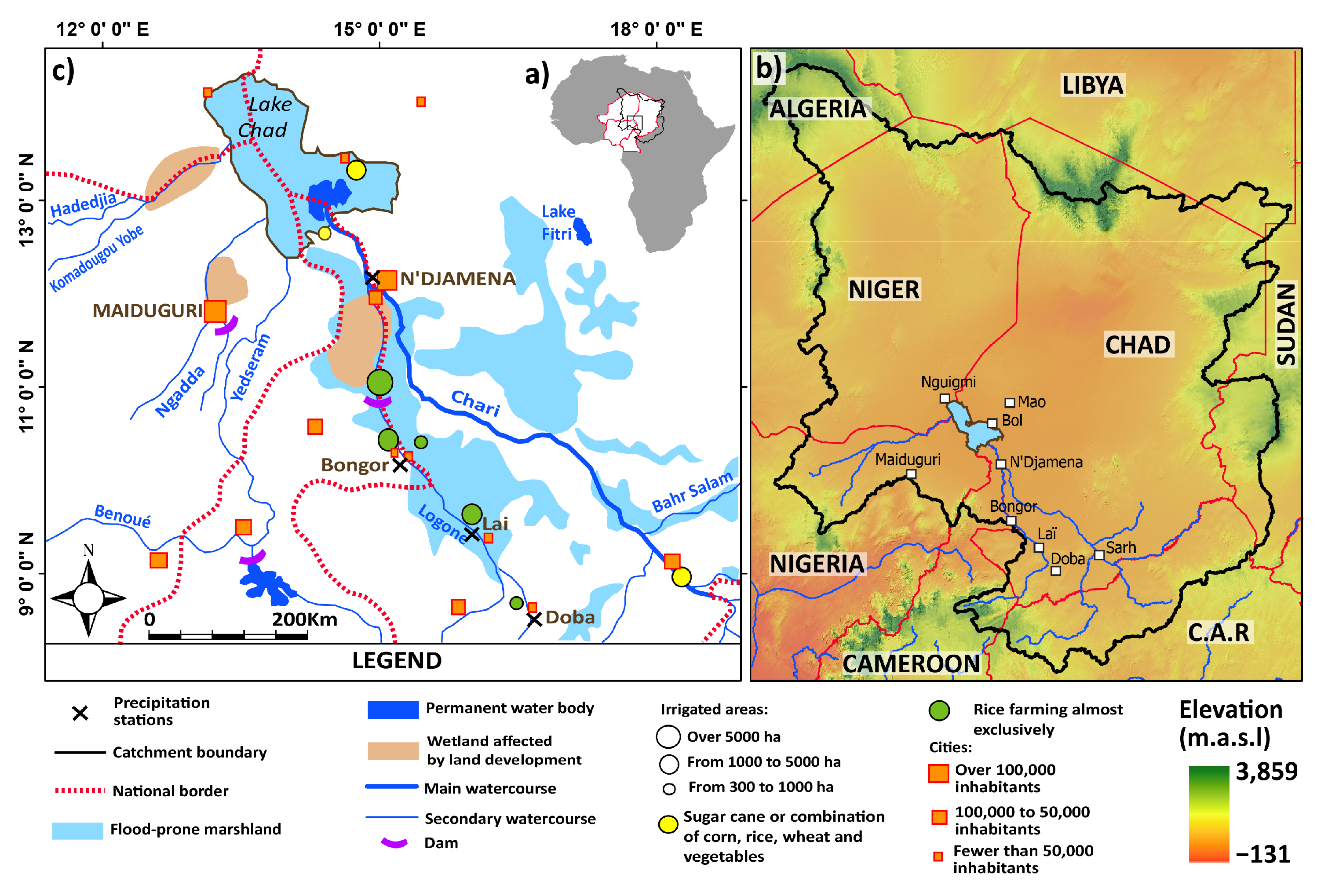
Figure 1.
(a) Location of Lake Chad within Niger, Nigeria, Cameroon, Chad and their position in relation to Africa. (b) The zoomed LCB with riparian countries, where C.A.R stands for the Central African Republic. (c) The major and secondary water courses that feed lake Chad, neighbouring permanent water bodies and dams used for irrigation/domestic supply, local city names and locations with over 100,000 inhabitants (location only for cities with fewer than 100,000 inhabitants), irrigation areas and relative field sizes as well as common agricultural crops grown in the region, as well as the precipitation gauges considered in the study.
Figure 2.
Contrast between a classical reccurrent neural network cell equipped with an activation function (A) and a memory block for LSTM artificial neural network [
39].
Figure 2.
Contrast between a classical reccurrent neural network cell equipped with an activation function (A) and a memory block for LSTM artificial neural network [
39].
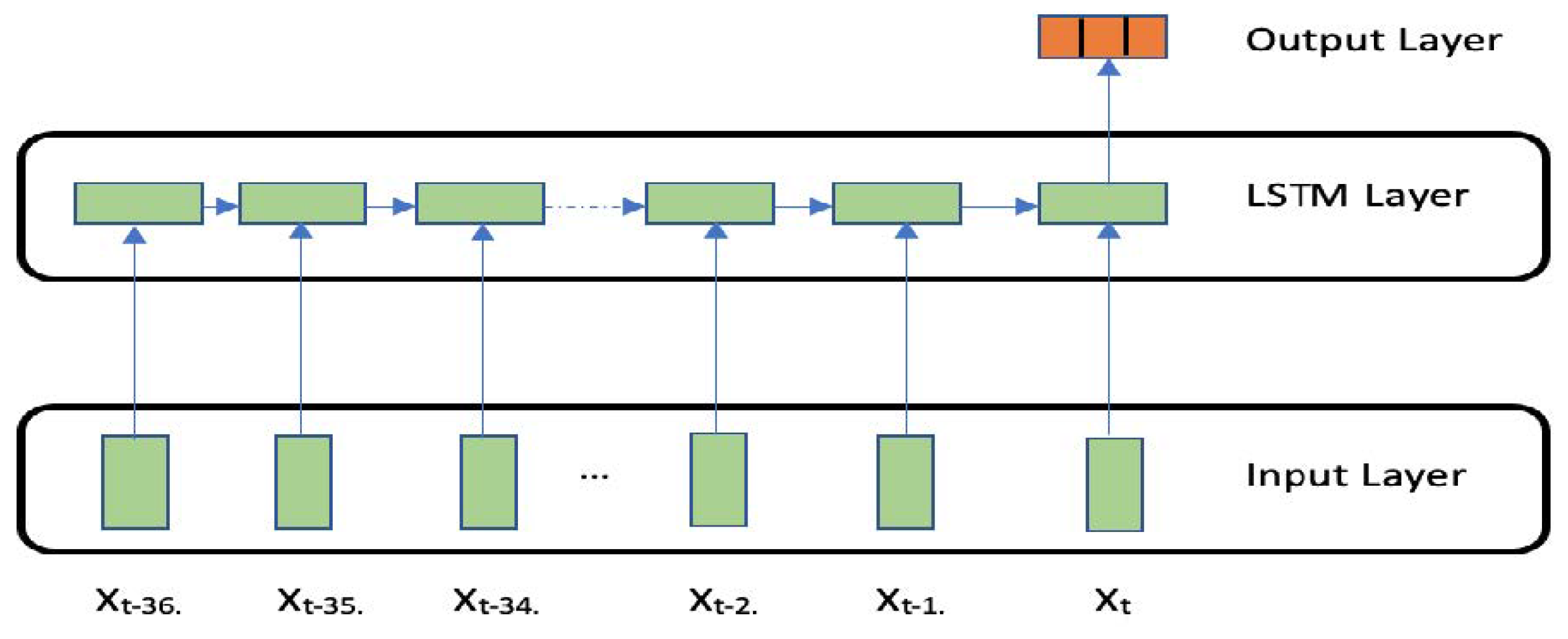
Figure 3.
The general architecture of the proposed LSTM networks implemented for both the precipitations and temperatures forecasting.
Figure 3.
The general architecture of the proposed LSTM networks implemented for both the precipitations and temperatures forecasting.
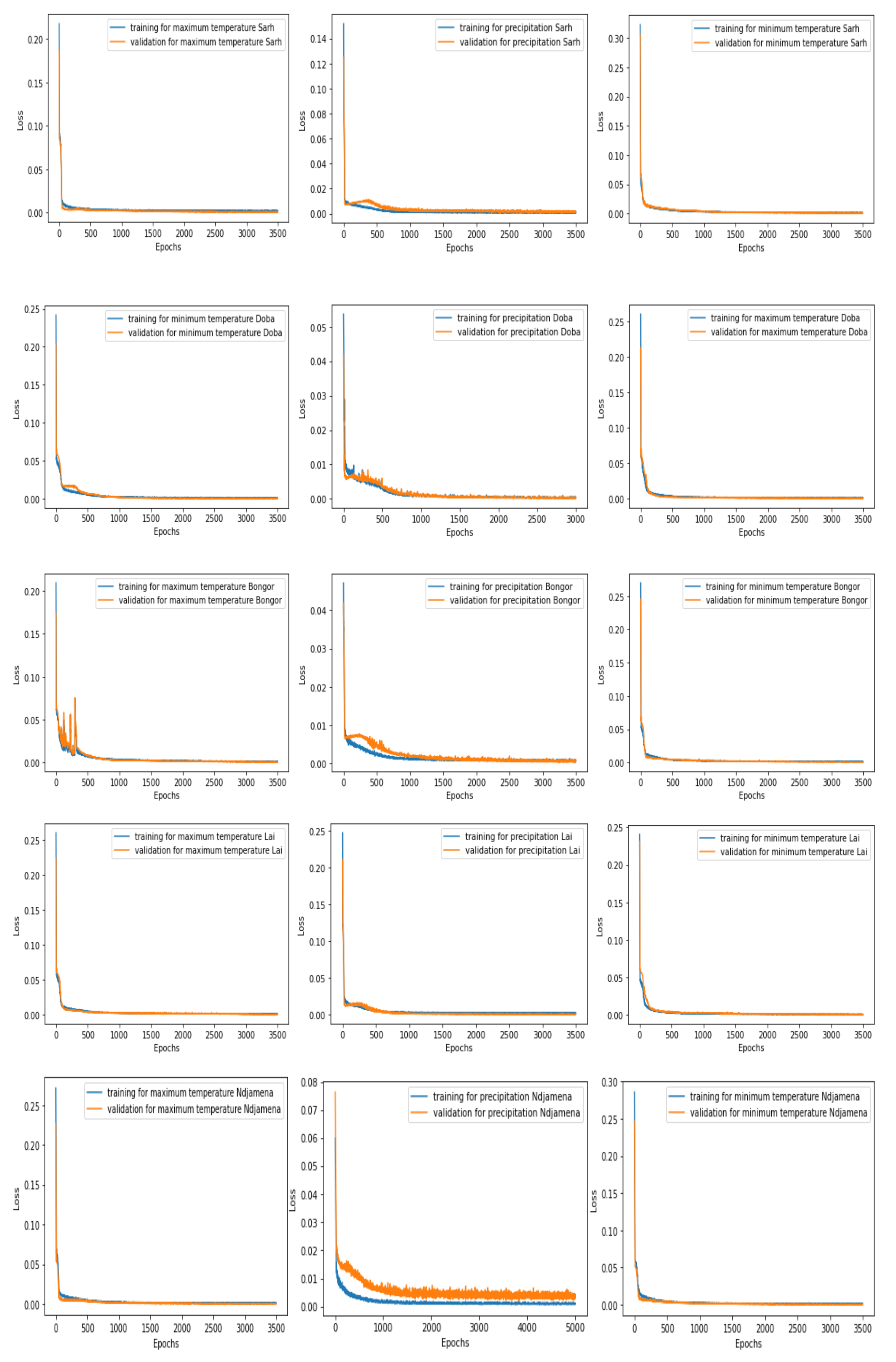
Figure 4.
The training and validation loss function plots for the maximum and minimum temperature and precipitation forecasting for the five gauging stations.
Figure 4.
The training and validation loss function plots for the maximum and minimum temperature and precipitation forecasting for the five gauging stations.
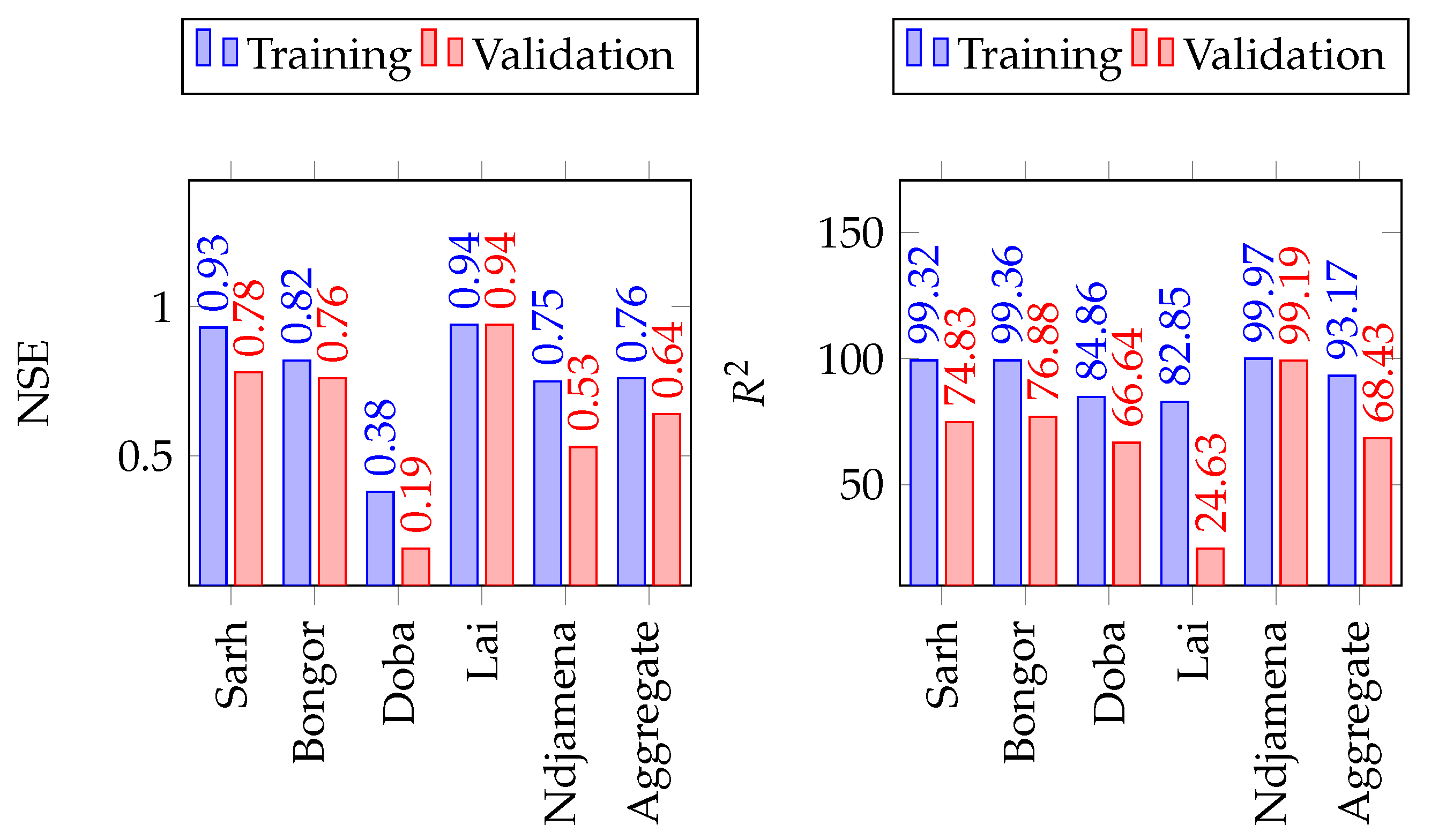
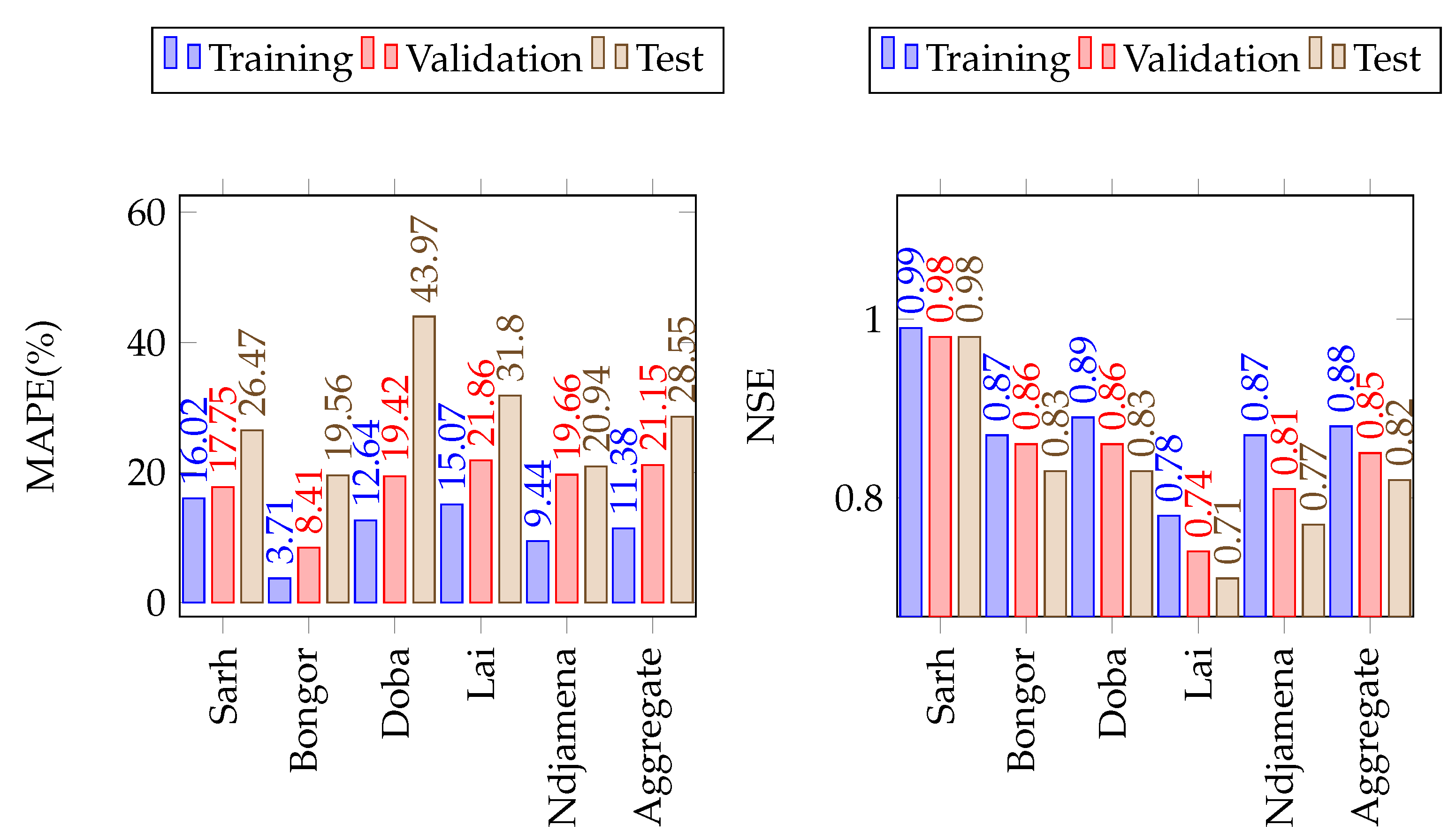
Figure 5.
Comparison of SDSM performance on the training and validation sets for monthly precipitations forecast in the Lake Chad Basin.
Figure 5.
Comparison of SDSM performance on the training and validation sets for monthly precipitations forecast in the Lake Chad Basin.
Figure 6.
Comparison of SDSM performance on the training and validation sets for monthly minimum temperature forecast in the Lake Chad Basin.
Figure 6.
Comparison of SDSM performance on the training and validation sets for monthly minimum temperature forecast in the Lake Chad Basin.
Figure 7.
Comparison of SDSM performance on the training and validation sets for monthly maximum temperature forecast in the Lake Chad Basin.
Figure 7.
Comparison of SDSM performance on the training and validation sets for monthly maximum temperature forecast in the Lake Chad Basin.
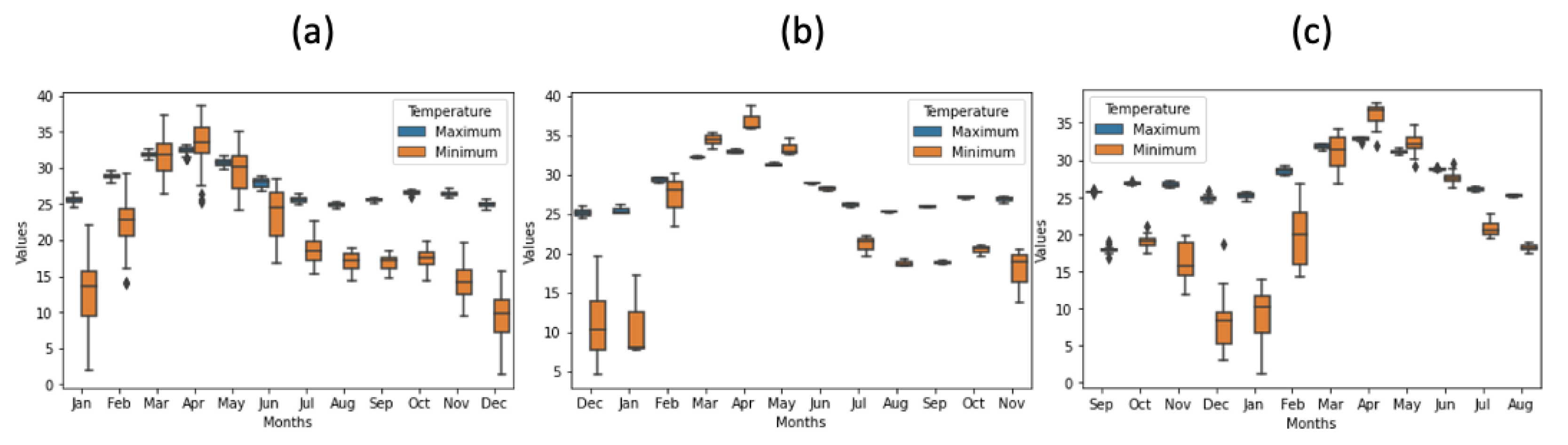
Figure 8.
Boxplot of monthly minimum and maximum temperatures data, displaying the heterogeneous spread in (a) the training, (b) the validation and (c) the test sets.
Figure 8.
Boxplot of monthly minimum and maximum temperatures data, displaying the heterogeneous spread in (a) the training, (b) the validation and (c) the test sets.
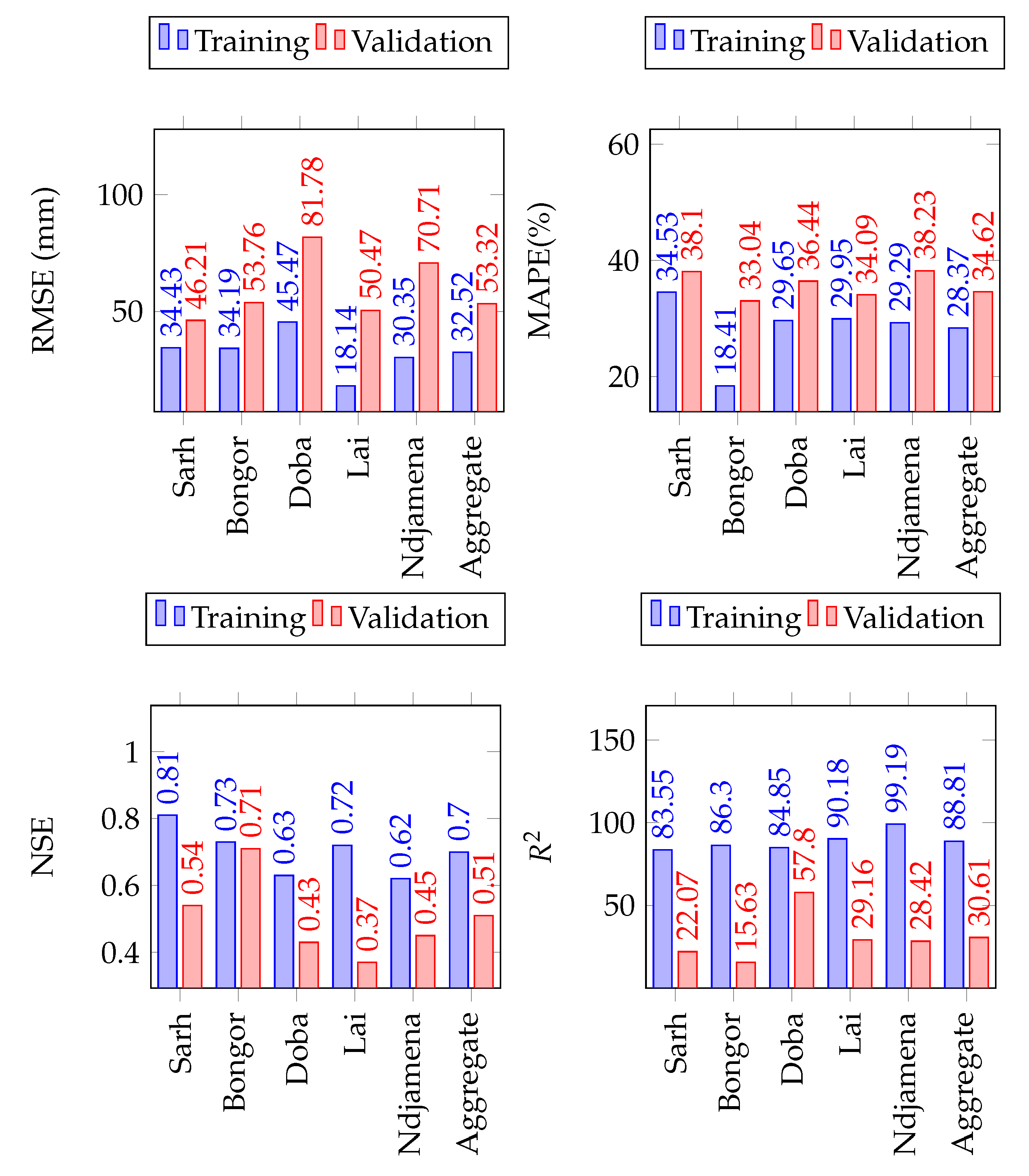
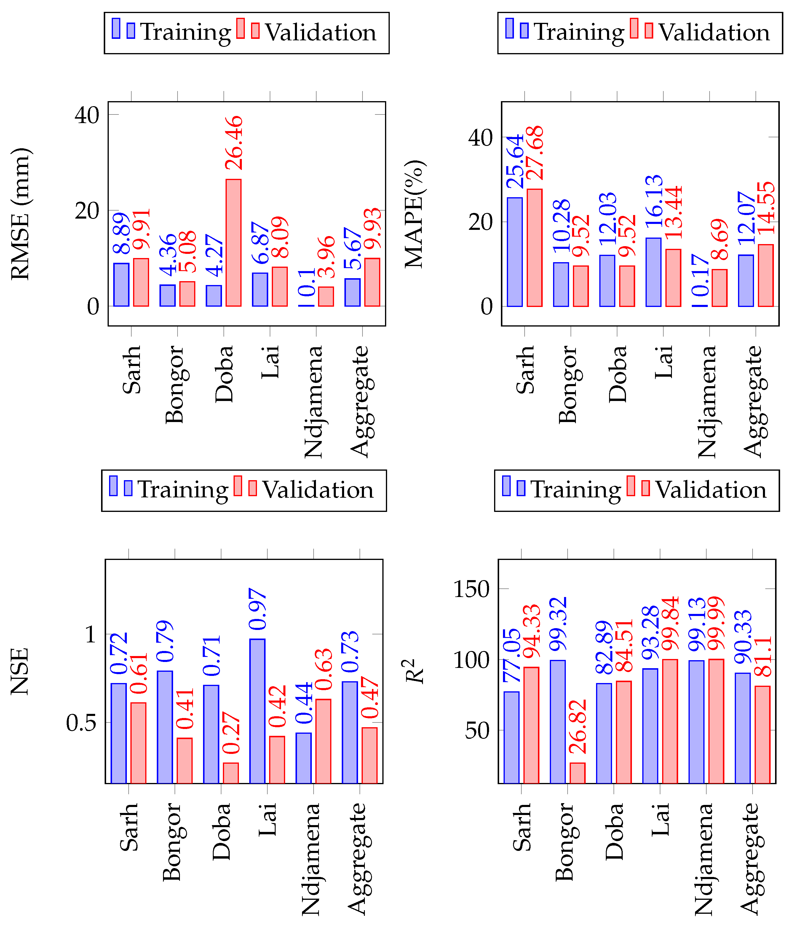
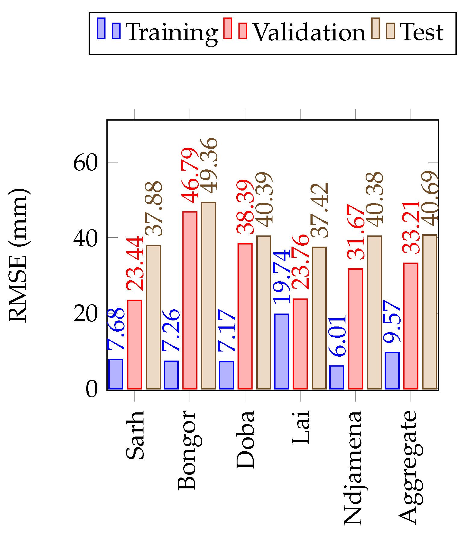
Figure 9.
The LSTM model performance on the training, validation and test sets of precipitation in the Lake Chad Basin. The number of simulations run were 20 in all cases.
Figure 9.
The LSTM model performance on the training, validation and test sets of precipitation in the Lake Chad Basin. The number of simulations run were 20 in all cases.
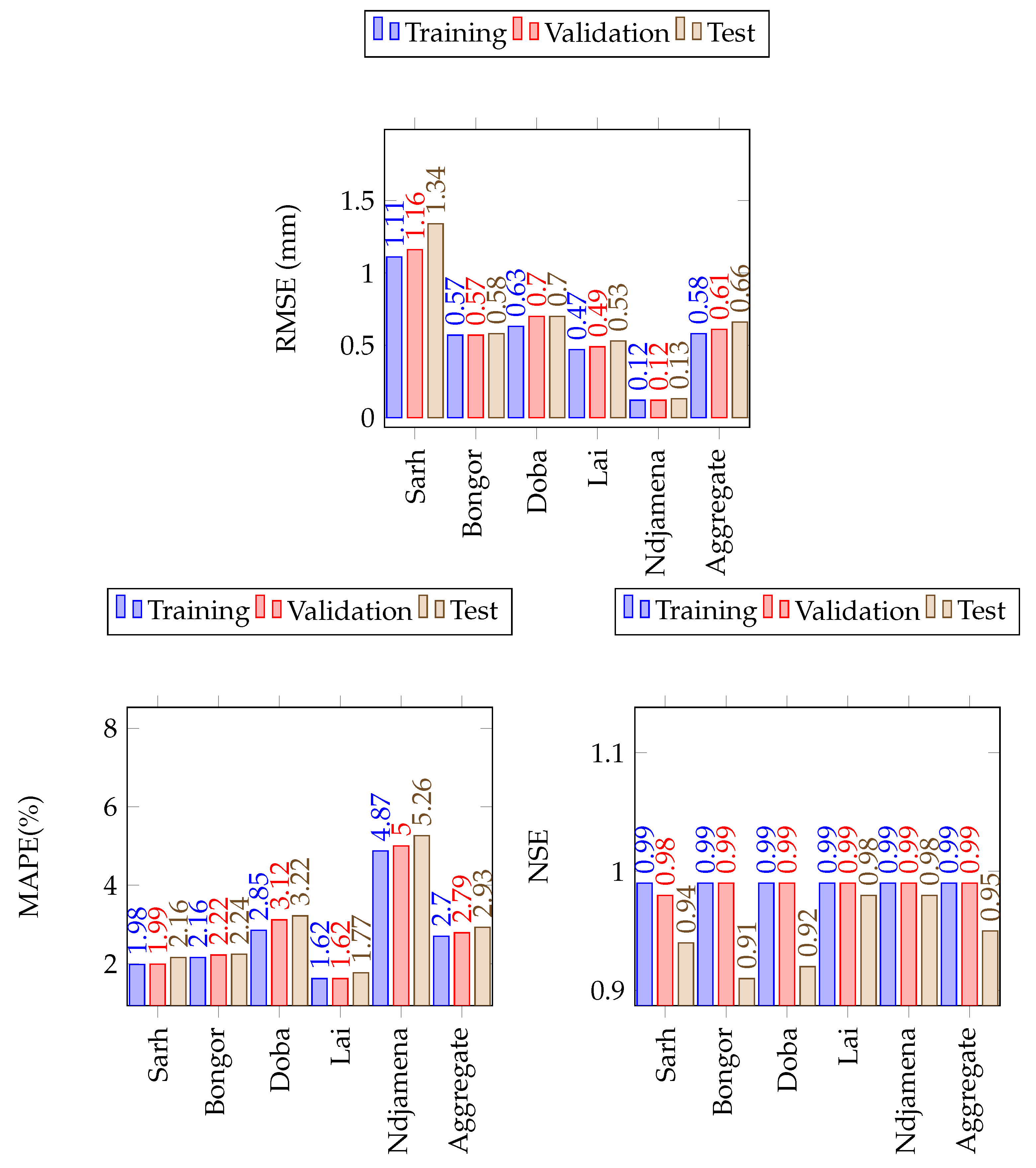
Figure 10.
The LSTM model performance on the training, validation and test sets of minimum temperature in the Lake Chad Basin. The number of simulations run were 20 in all cases.
Figure 10.
The LSTM model performance on the training, validation and test sets of minimum temperature in the Lake Chad Basin. The number of simulations run were 20 in all cases.
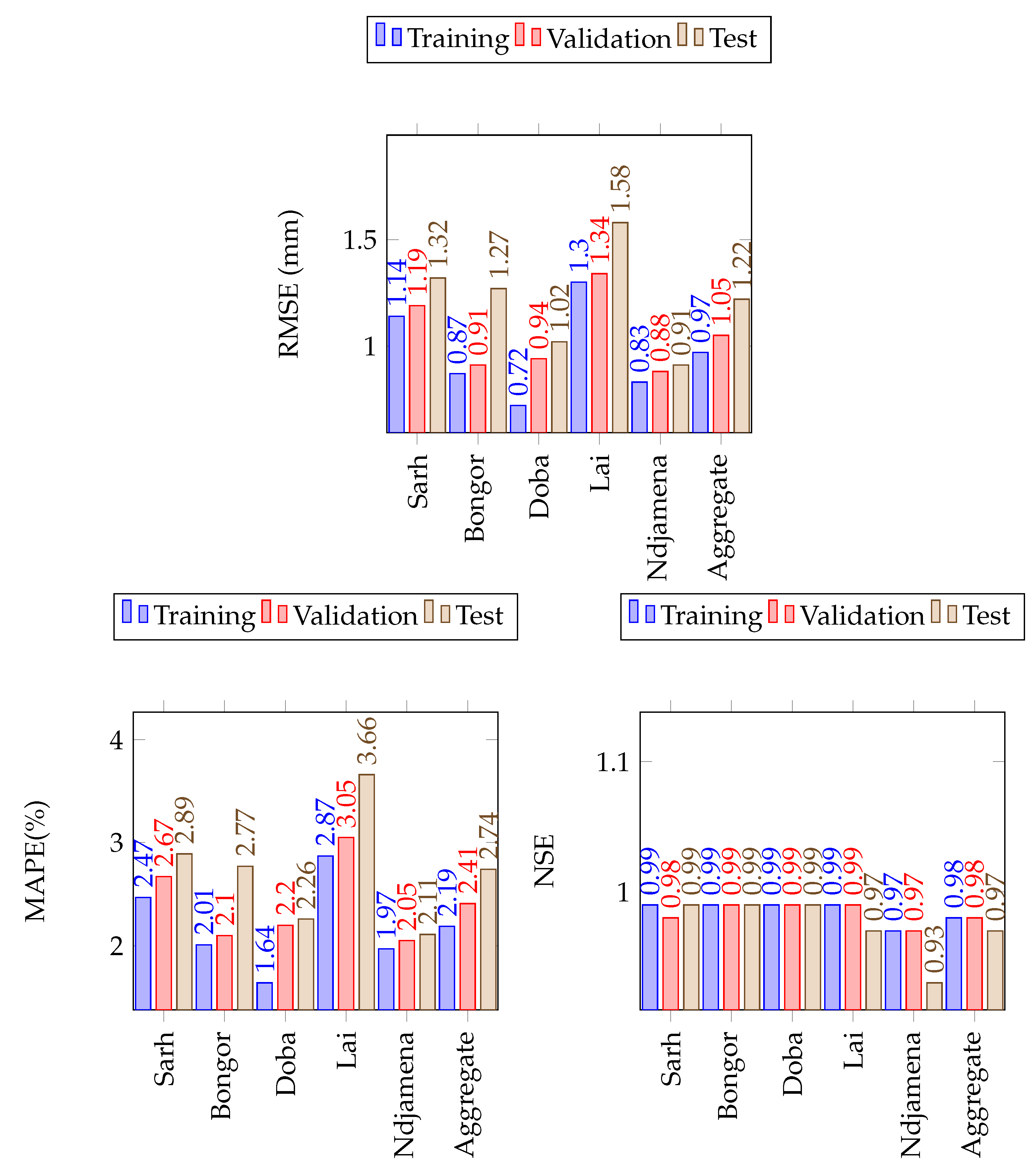
Figure 11.
The LSTM model performance on the training, validation and test sets of maximum temperature in the Lake Chad Basin. The number of simulations run were 20 in all cases.
Figure 11.
The LSTM model performance on the training, validation and test sets of maximum temperature in the Lake Chad Basin. The number of simulations run were 20 in all cases.
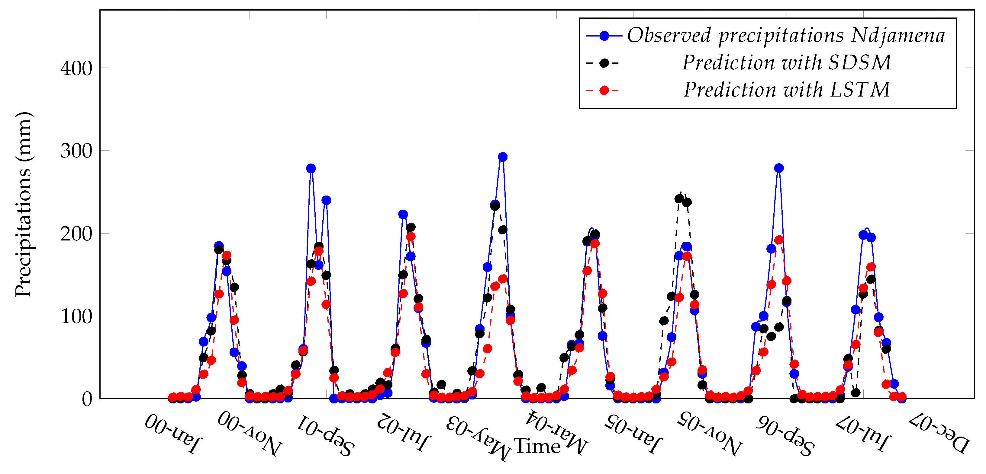
Figure 12.
Observed and predicted precipitation in Ndjamena.
Figure 12.
Observed and predicted precipitation in Ndjamena.
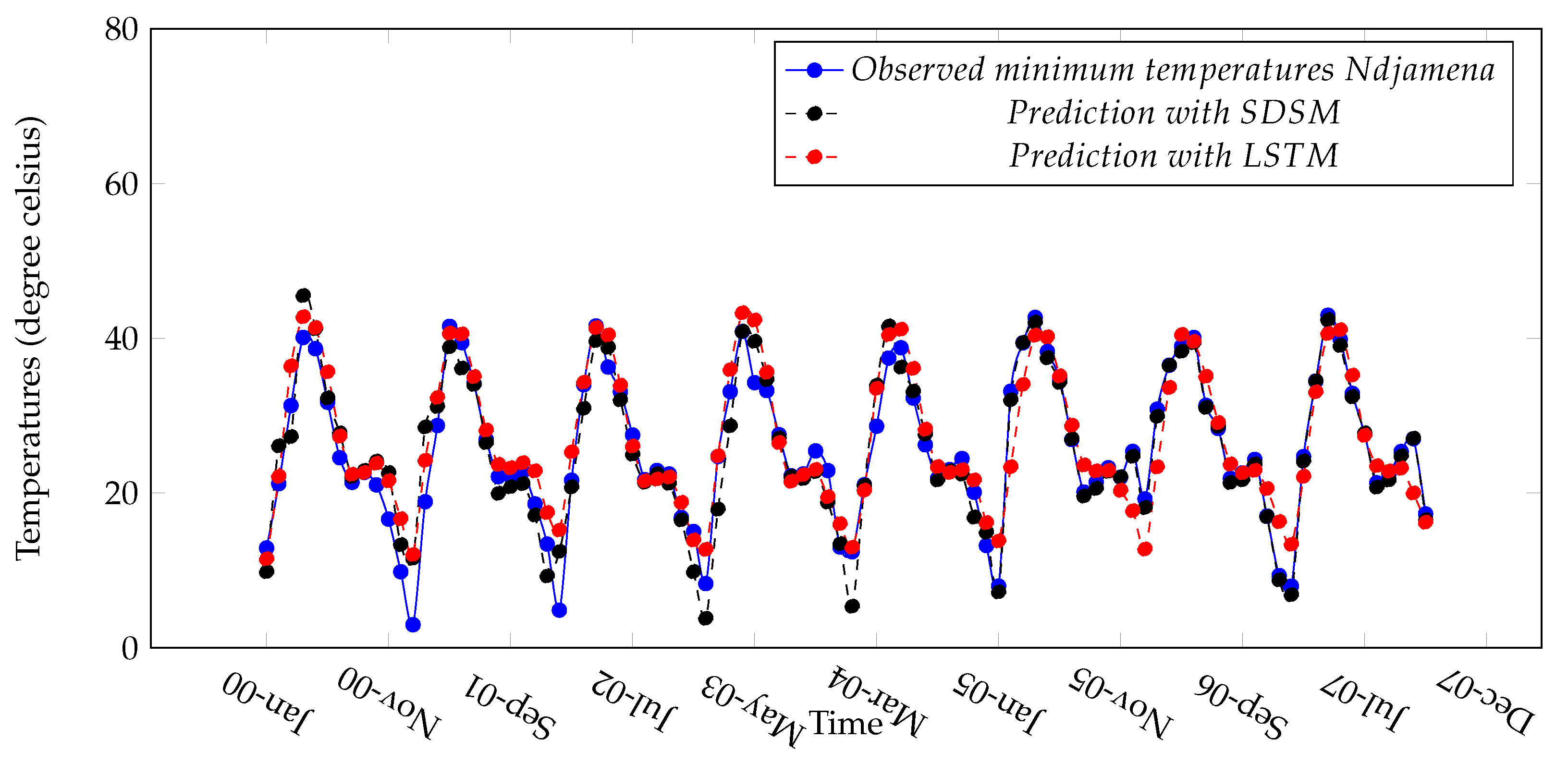
Figure 13.
Observed and predicted minimum temperature in Ndjamena.
Figure 13.
Observed and predicted minimum temperature in Ndjamena.
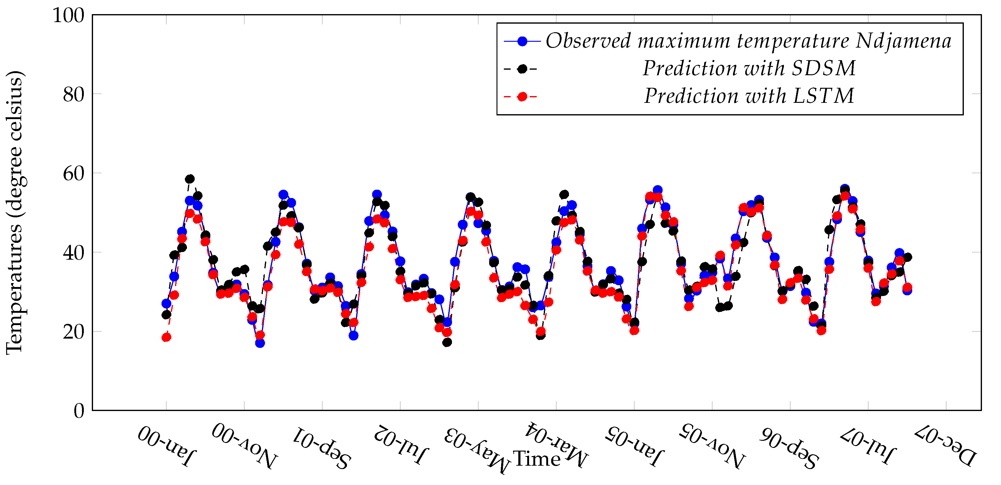
Figure 14.
Observed and predicted maximum temperature in Ndjamena.
Figure 14.
Observed and predicted maximum temperature in Ndjamena.
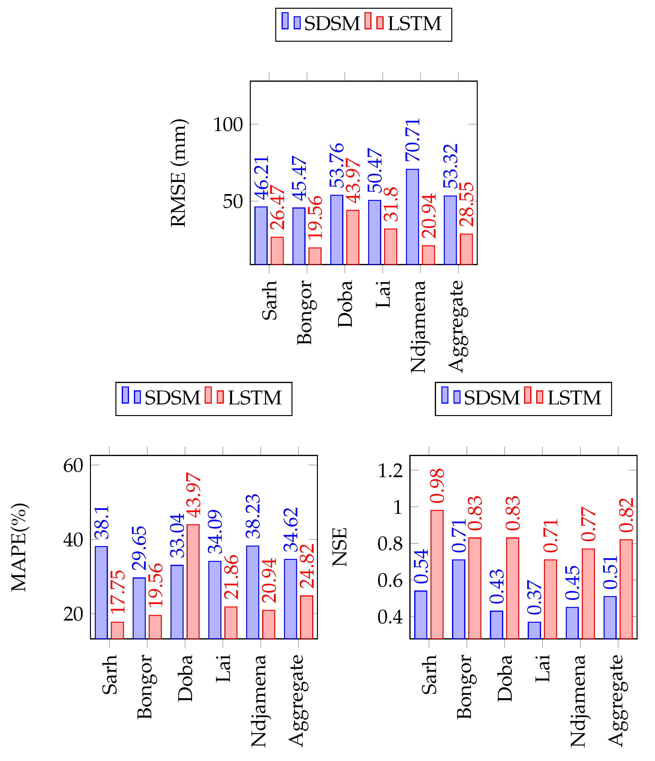
Figure 15.
Comparison of SDSM & LSTM for monthly precipitations forecast in the Lake Chad Basin.
Figure 15.
Comparison of SDSM & LSTM for monthly precipitations forecast in the Lake Chad Basin.
Figure 16.
SDSM and LSTM forecasting performance comparison for monthly minimum temperature forecast.
Figure 16.
SDSM and LSTM forecasting performance comparison for monthly minimum temperature forecast.
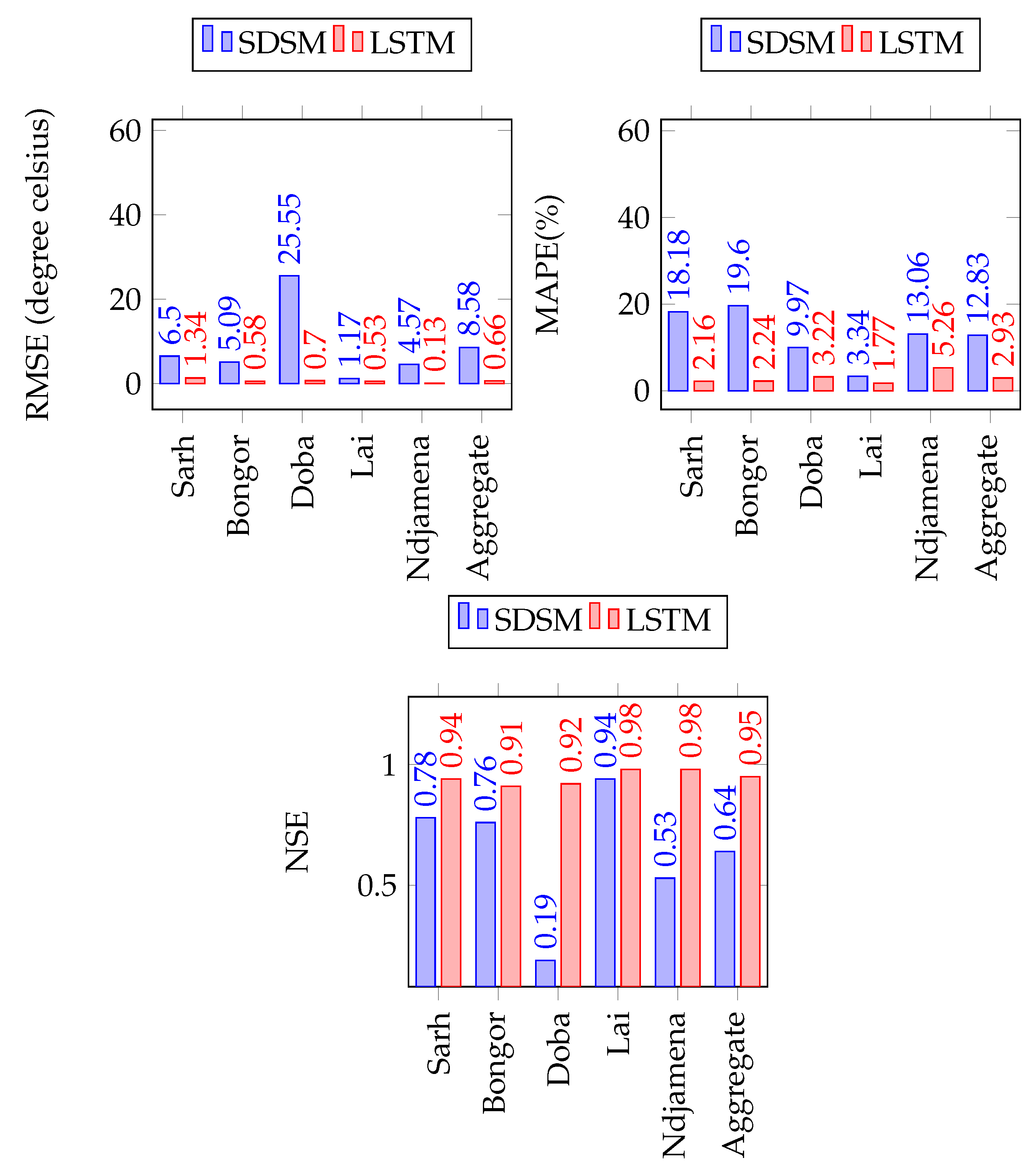
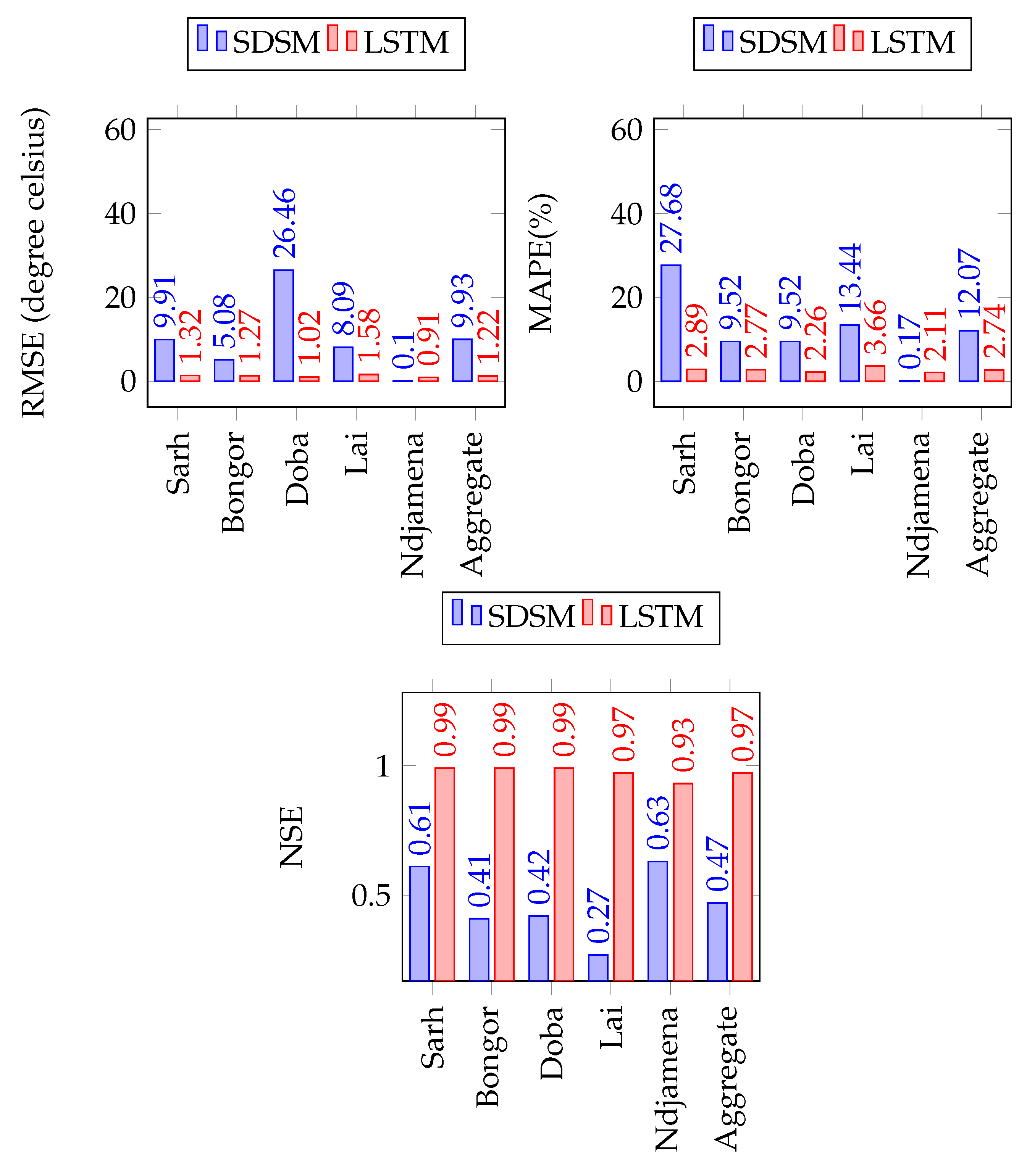
Figure 17.
SDSM and LSTM forecasting performance comparison for monthly maximum temperature forecast.
Figure 17.
SDSM and LSTM forecasting performance comparison for monthly maximum temperature forecast.
Table 1.
Data subsets for the purpose of comparison between SDSM and LSTM implementation in the Lake Chad Basin. The validation set of the SDSM implementation correspond to the test set of the LSTM subset.
Table 1.
Data subsets for the purpose of comparison between SDSM and LSTM implementation in the Lake Chad Basin. The validation set of the SDSM implementation correspond to the test set of the LSTM subset.
| Methods | SDSM | LSTM |
|---|
| Subset Names | Calibration | Validation | Training | Validation | Test |
| Years | 1950–2004 | 2005–2007 | 1950–1990 | 1991–2004 | 2005–2007 |
| Data Allocated (%) | | | | | |
Table 2.
Definition of variable names, their units and corresponding models. °N denotes North direction, mm denotes Millimeter, and * denotes dimensionless Z-score. (a) denotes monthly precipitation model, (b) denotes monthly minimum temperatures and (c) denotes monthly maximum temperatures model.
Table 2.
Definition of variable names, their units and corresponding models. °N denotes North direction, mm denotes Millimeter, and * denotes dimensionless Z-score. (a) denotes monthly precipitation model, (b) denotes monthly minimum temperatures and (c) denotes monthly maximum temperatures model.
| Variable | Definition | Units | Model |
|---|
| Min temp | Minimum temperatures | degree celsius | (c) |
| Max_temp | Maximum temperatures | degree celsius | (b) |
| dswr | Direct shortwave radiation | * | (a,b,c) |
| lftx | Surface lifted index | * | (a) |
| p_u | Zonal velocity component near the surface | * | (a) |
| p_th | Wind direction near the surface | °N | (a) |
| p5_f | Geostrophic airflow velocity at 500 hPa | * | (a) |
| p5_u | Zonal velocity component at 500 hPa | * | (a) |
| p5_z | Vorticity at 500 hPa | * | (a) |
| p5th | Wind direction at 500 hPa | °N | (a) |
| p8_u | Zonal velocity component at 850 hPa | * | (a) |
| p8th | Wind direction at 850 hPa | °N | (a) |
| pr_wtr | Precipitable water | * | (a) |
| ncepprec | Large scale precipitations | mm | (a) |
| r500 | Large scale precipitations | * | (a) |
| r850 | Relative humidity at 500 hpa height | * | (a) |
| rhum | Relative humidity at 850 hpa height | * | (a) |
| shum | Near surface relative humidity | * | (a) |
| mslp | Mean sea level pressure | * | (b,c) |
| p_z | Vorticity near the surface | * | (b,c) |
| pottmp | Potential temperature | * | (b,c) |
| p500 | 500 hpa geopotential height | * | (b,c) |
Table 3.
Architectures and hyperparameters investigated for monthly precipitation and temperatures forecasting.
Table 3.
Architectures and hyperparameters investigated for monthly precipitation and temperatures forecasting.
| Hyperparameter & Architecture | Options Explored | Best Selections |
|---|
| Window size | 1, 2, …, 12, 24, 36 | 36 |
| Hidden Nodes | 5, 10, 15, 20, 25, 30, 35 | 15, 20 |
| Optimizers | adam, adagrad, sgd, adadelta, Nadam | adam |
| LearningRates | 0.1, 0.01, 0.001, 0.09, 0.2 | 0.01 |
| Dropouts | 0.09, 0.1, 0.2, 0.3, 0.4, 0.5 | 0.09, 0.2 |
| Batch sizes | 4, 5, 10, 20, 25, 30 | 5, 10, 15 |
| Epochs | 100, 200, 500, 1000, 2000, 2500, 3000 | 2500, 3000 |
Table 4.
The chosen LSTM architectures for precipitation, minimum and maximum temperature forecasting in the five gauging stations after hyperparameter tuning.
Table 4.
The chosen LSTM architectures for precipitation, minimum and maximum temperature forecasting in the five gauging stations after hyperparameter tuning.
| | Window Size | Nodes | Epochs | Hidden Layers | Optimiser | Dropout | Batch Size | Simulations |
|---|
| Precipitation | | | | | | | | |
| Sarh | 36 | 20 | 3000 | 1 | adam | 0.09 | 4 | 20 |
| Bongor | 36 | 15 | 3000 | 1 | adam | 0.2 | 10 | 20 |
| Doba | 36 | 20 | 2500 | 1 | adam | 0.09 | 5 | 20 |
| Lai | 36 | 15 | 3000 | 1 | adam | 0.2 | 10 | 20 |
| Ndjamena | 36 | 15 | 3000 | 1 | adam | 0.2 | 10 | 20 |
| Minimum temperature | | | | | | | | |
| Sarh | 36 | 15 | 3000 | 1 | adam | 0.2 | 10 | 20 |
| Bongor | 36 | 15 | 3000 | 1 | adam | 0.2 | 10 | 20 |
| Doba | 36 | 15 | 3000 | 1 | adam | 0.2 | 10 | 20 |
| Lai | 36 | 15 | 2500 | 1 | adam | 0.2 | 10 | 20 |
| Ndjamena | 36 | 15 | 3000 | 1 | adam | 0.2 | 10 | 20 |
| Maximum temperature | | | | | | | | |
| Sarh | 36 | 15 | 3000 | 1 | adam | 0.2 | 10 | 20 |
| Bongor | 36 | 15 | 3000 | 1 | adam | 0.2 | 10 | 20 |
| Doba | 36 | 15 | 2500 | 1 | adam | 0.2 | 5 | 20 |
| Lai | 36 | 15 | 2500 | 1 | adam | 0.2 | 10 | 20 |
| Ndjamena | 36 | 15 | 3000 | 1 | adam | 0.2 | 10 | 20 |
Table 5.
The statistical difference of the mean and variance estimation for the five gauging stations between the training, validation and test sets. p-values are given in brackets.
Table 5.
The statistical difference of the mean and variance estimation for the five gauging stations between the training, validation and test sets. p-values are given in brackets.
| | Training vs. Validation | Validation vs. Test | Training vs. Test |
|---|
| | | | | | | |
|---|
| | Sarh |
| MaxTemp | −0.14 (0.55) | −0.15 (0.91) | −0.19 (0.70) | −0.47 (0.81) | −0.33 (0.47) | −0.62 (0.76) |
| MinTemp | −0.67 (0.35) | −13.76 (0.22) | −1.66 (0.29) | −4.97 (0.78) | −2.33(0.08) | −18.72 (0.33) |
| Precipitation | 2.73 (0.72) | 62.30 (0.53) | −0.12 (0.99) | −99.79 (0.88) | 2.62 (0.86) | 566.50 (0.86) |
| | Bongor |
| MaxTemp | −0.34 (0.73) | −3.90 (0.99) | −2.04 (0.31) | −5.68 (0.71) | −2.38 (0.20) | −9.58 (0.70) |
| MinTemp | −0.33 (0.72) | −11.75 (0.56) | −2 (0.31) | −1.26 (0.92) | −2.33 (0.19) | −13.01 (0.68) |
| Precipitation | −3.55 (0.66) | −1864 (0.63) | −2.62 (0.68) | 850.40 (0.80) | −6.18 (0.88) | −1013.94 (0.57) |
| | Doba |
| MaxTemp | −0.14 (0.55) | −0.15 (0.92) | −0.19 (0.70) | −0.47 (0.81) | −0.33 (0.47) | −0.62 (0.76) |
| MinTemp | −6.67 (0.35) | −13.76 (0.22) | −1.66 (0.29) | −4.97 (0.78) | −2.33 (0.08) | −18.72 (0.33) |
| Precipitation | 2.22 (0.81) | 871.38 (0.83) | 0.08 (0.99) | 91.55 (0.96) | 2.30 (0.89) | 962.93 (0.95) |
| | Lai |
| MaxTemp | −1.90 (0.19) | −33.51 (0.52) | −3.78 (0.23) | −35.44 (0.47) | −5.68 (0.04) | −68.95 (0.24) |
| MinTemp | −1.92 (0.16) | −56.58 (0.15) | −3.65 (0.23) | −18.63 (0.74) | −5.57 (0.03) | −75.22 (0.25) |
| Precipitation | 0.29 (0.96) | −14.31 (0.90) | −0.29 (0.98) | −243.09 (0.88) | −0.005 (0.99) | −257.39 (0.82) |
| | Ndjamena |
| MaxTemp | −0.36 (0.70) | 15.2 (0.24) | −1.36 (0.45) | −1.64 (0.91) | −1.73 (0.35) | 13.56 (0.61) |
| MinTemp | −0.39 (0.67) | 8.92 (0.32) | −1.31 (0.45) | 1.08 (0.99) | −1.70 (0.32) | 10.01 (0.59) |
| Precipitation | −3.26 (0.62) | −843 (0.60) | −3.05 (0.82) | −45.27 (0.78) | −6.31 (0.60) | −888.28 (0.55) |
Table 6.
Monthly predictions biases and monthly correlations between observed and predicted values.
Table 6.
Monthly predictions biases and monthly correlations between observed and predicted values.
| Precipitation |
|---|
| | Error | Correlation |
|---|
| | sdsm | lstm | sdsm | lstm |
|---|
| January | 11.47 | 1.34 | 0.33 | 0.92 |
| February | 11.46 | 1.32 | 0.33 | 0.75 |
| March | −3.22 | −4.26 | 0.55 | 0.96 |
| April | −8.11 | −13.17 | 0.74 | 0.85 |
| May | 19.52 | −1.48 | 0.25 | 0.77 |
| June | 34.57 | 13.93 | 0.65 | 0.83 |
| July | 72.84 | 37.81 | 0.01 | 0.84 |
| August | 28.89 | 25.63 | 0.40 | 0.83 |
| September | 3.23 | −5.65 | 0.64 | 0.94 |
| October | 7.67 | 1.91 | 0.55 | 0.88 |
| November | −1.28 | −3.69 | 0.57 | 0.91 |
| December | −1.95 | −3.61 | 0.88 | 0.91 |
| Minimum Temperature |
| | Error | Correlation |
| | sdsm | lstm | sdsm | lstm |
| January | −1.30 | 0.12 | 0.36 | 0.82 |
| February | −1.29 | 0.09 | 0.52 | 0.72 |
| March | −0.90 | 0.45 | 0.63 | 0.74 |
| April | −0.49 | −0.39 | 0.08 | 0.89 |
| May | −2.64 | −0.29 | 0.21 | 0.90 |
| June | −2.29 | −0.07 | 0.77 | 0.76 |
| July | −0.75 | −0.22 | 0.04 | 0.74 |
| August | −1.35 | 0.44 | 0.53 | 0.80 |
| September | −0.16 | 0.60 | 0.86 | 0.87 |
| October | 0.53 | 0.74 | 0.25 | 0.95 |
| November | −0.51 | 0.36 | 0.67 | 0.85 |
| December | −1.73 | 0.68 | 0.96 | 0.92 |
| Maximum Temperature |
| | Error | Correlation |
| | sdsm | lstm | sdsm | lstm |
| January | 2.38 | 0.77 | 0.01 | 0.89 |
| February | 2.30 | 1.18 | 0.25 | 0.93 |
| March | 2.53 | 1.87 | 0.01 | 0.90 |
| April | 6.83 | 3.01 | 0.05 | 0.74 |
| May | 6.69 | 2.25 | 0.24 | 0.75 |
| June | 1.51 | 0.01 | 0.56 | 0.77 |
| July | 2.20 | 0.03 | 0.59 | 0.75 |
| August | 1.09 | −0.01 | 0.35 | 0.87 |
| September | 0.92 | 0.05 | 0.35 | 0.91 |
| October | 3.05 | 0.20 | 0.01 | 0.85 |
| November | 3.17 | −0.20 | 0.06 | 0.75 |
| December | 1.51 | 1.69 | 0.91 | 0.97 |


