
Machine Learning-Aided Remote Monitoring of NOx Emissions from Heavy-Duty Diesel Vehicles Based on OBD Data Streams
 ,
,
Abstract
:1. Introduction
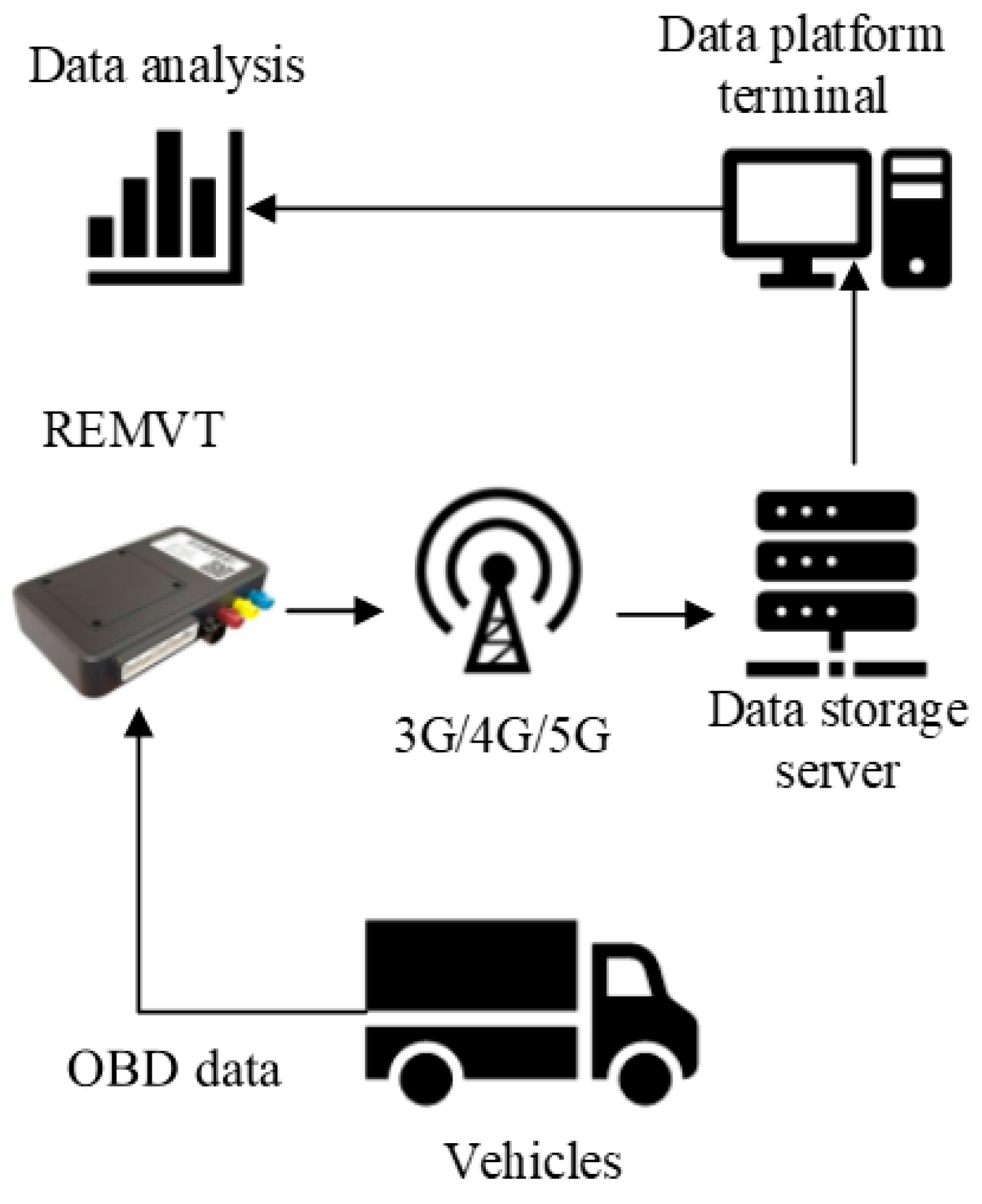
2. OBD Resource
2.1. Test Vehicle and Route Information
2.2. Test Equipment
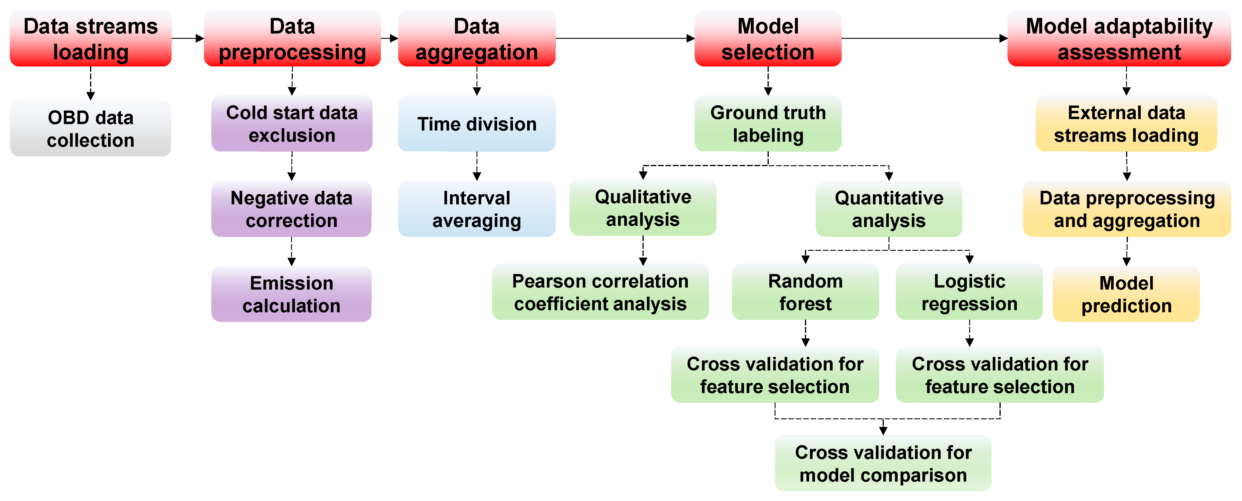
3. Data Process and Methodology
3.1. Data Preprocessing
- Cold-start data exclusion: Remove cold-start data with engine coolant temperatures less than 70 °C.
- Negative data correction: In the case of the actual torque percentage being less than the frictional torque percentage due to occasional, random fluctuations of the sensors, set both percentages to zero. Set negative readings of the NOx concentration (also caused by sensor drift) to zero.
- Emission calculation: Sequentially calculate the instantaneous torque, engine work, NOx emissions and specific NOx emissions from the calibrated data.
3.2. Data Aggregation
- Enhancing independence within the data: After data aggregation, there is far less correlation between the one-minute samples, which better fits the basic assumptions of most current machine learning methodologies.
- Removing the burden of inefficient computation from the model: Through data aggregation, redundant information in the original sequence is greatly compressed, and the number of one-minute samples requires far fewer computing resources for the model training and validation.
- Improving the normality of the data distribution: According to the central limit theorem, the aggregated data approach a normal distribution regardless of the skewness and kurtosis of the distribution of the original sequence, which benefits the robustness of the model inference.
- Reducing the influence of outliers: The potential outliers that emerge due to the uncertainty of the indications are smoothed out by averaging, which further ensures the robustness of the model training.
3.3. Ground Truth Labeling
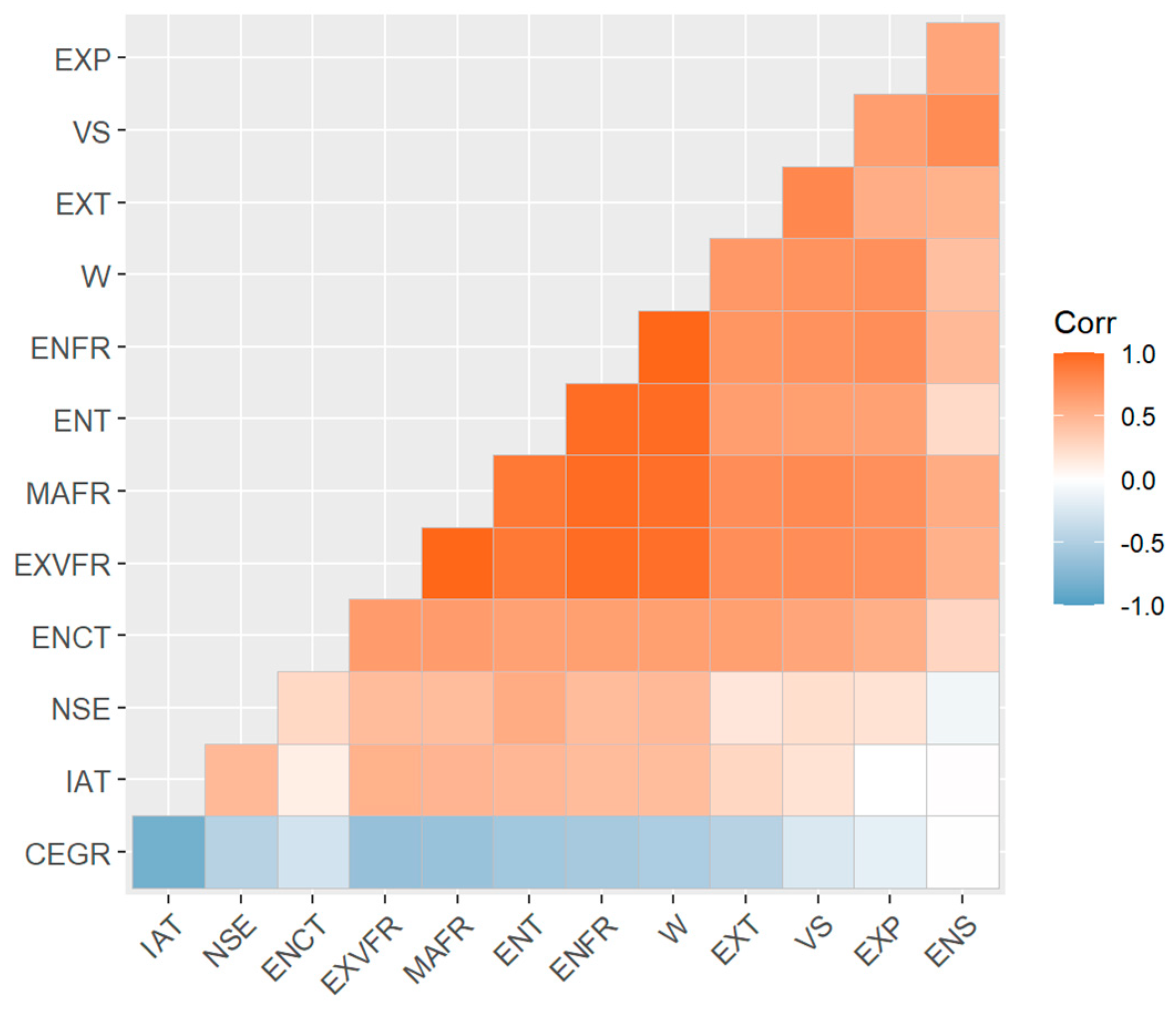
3.4. Correlation Coefficient Analysis
3.5. Modeling and Evaluation Design
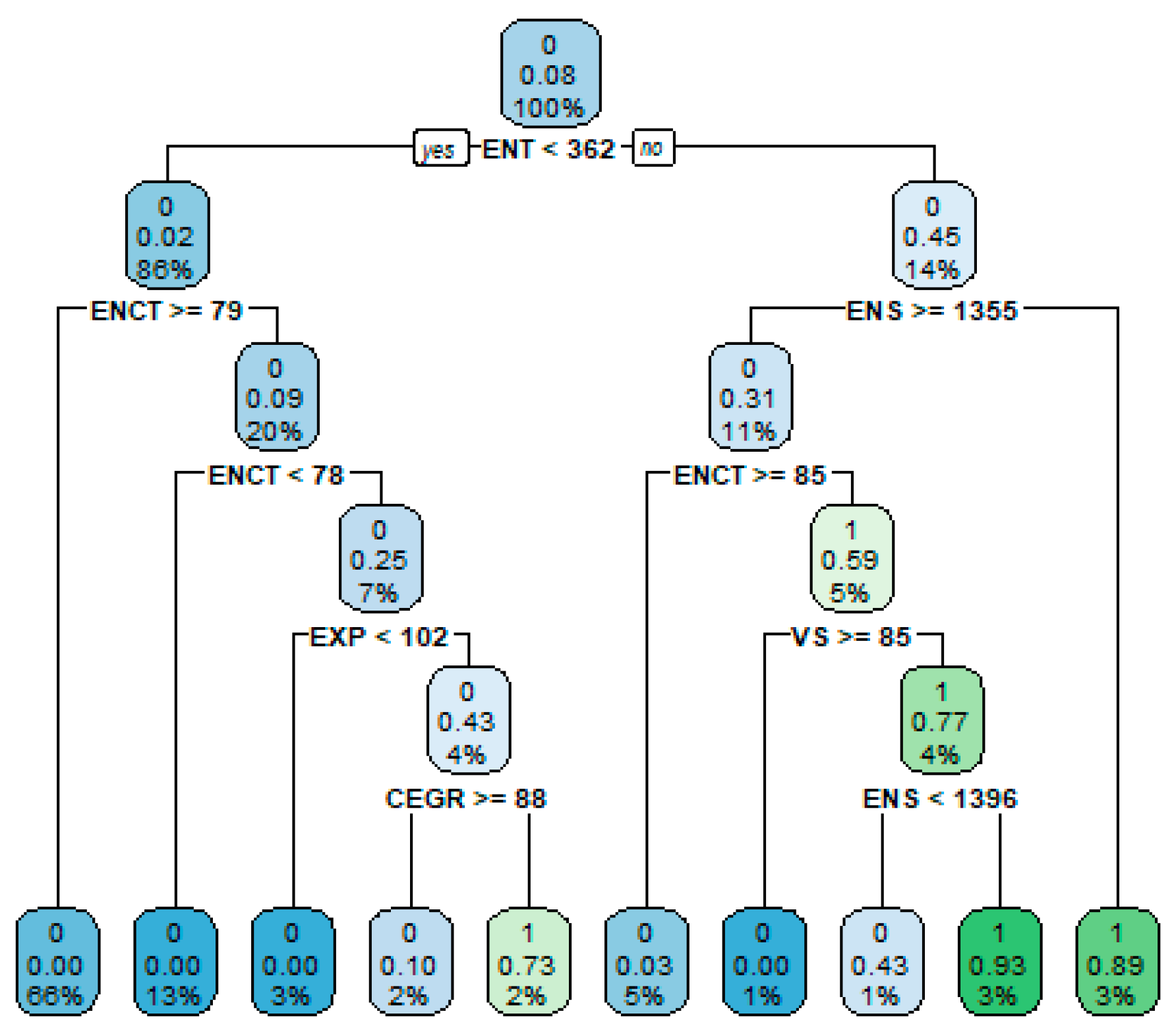
3.5.1. Random Forest
3.5.2. Logistic Regression
4. Results and Discussions
4.1. Model Comparison through Cross-Validation
4.2. Trials for More Precision
5. Model Adaptability Assessment Using External Data
6. Conclusion and Recommendations
Author Contributions
Funding
Institutional Review Board Statement
Informed Consent Statement
Data Availability Statement
Conflicts of Interest
References
- MEE (Ministry of Ecology and Environment P.R. China). China Mobile Source Environmental Management Annual Report (2022). 2021. Available online: https://www.vecc.org.cn/dbfile.svl?n=/u/cms/jdchbw/202212/09170954wf3x.pdf (accessed on 22 February 2023).
- MEE (Ministry of Ecology and Environment P.R. China); SAMR (State Administration for Market Regulation). Limits and Measurement Methods for Emissions from Diesel Fuelled Heavy-Duty Vehicles (CHINA VI); China Environmental Science Press: Beijing, China, 2018.
- Sun, Y.; Guo, Y.; Wang, C. Research on Data Consistency of Remote Emission Management Vehicle Terminals for Heavy-Duty Vehicles. Small Intern. Combust. Engine Veh. Technol. 2019, 48, 1–6. [Google Scholar]
- Zhang, X.; Li, J.; Yang, Z.; Xie, Z.; Li, T. Accuracy Analysis of Carbon Emissions Measurement of Heavy Heavy-Duty Diesel Vehicles Based on Remote Data. China Environ. Sci. 2022, 42, 4565–4570. [Google Scholar]
- Zhang, S.; Zhao, P.; He, L.; Yang, Y.; Liu, B.; He, W.; Cheng, Y.; Liu, Y.; Liu, S.; Hu, Q. On-Board Monitoring (OBM) for Heavy-Duty Vehicle Emissions in China: Regulations, Early-Stage Evaluation and Policy Recommendations. Sci. Total Environ. 2020, 731, 139045. [Google Scholar] [CrossRef] [PubMed]
- Wang, J.; Wang, R.; Yin, H.; Wang, Y.; Wang, H.; He, C.; Liang, J.; He, D.; Yin, H.; He, K. Assessing Heavy-Duty Vehicles (HDVs) on-Road NOx Emission in China from on-Board Diagnostics (OBD) Remote Report Data. Sci. Total Environ. 2022, 846, 157209. [Google Scholar] [CrossRef]
- Mera, Z.; Fonseca, N.; Casanova, J.; López, J.-M. Influence of Exhaust Gas Temperature and Air-Fuel Ratio on NOx Aftertreatment Performance of Five Large Passenger Cars. Atmos. Environ. 2021, 244, 117878. [Google Scholar] [CrossRef]
- Giechaskiel, B.; Clairotte, M.; Valverde-Morales, V.; Bonnel, P.; Kregar, Z.; Franco, V.; Dilara, P. Framework for the Assessment of PEMS (Portable Emissions Measurement Systems) Uncertainty. Environ. Res. 2018, 166, 251–260. [Google Scholar] [CrossRef]
- Feist, M.D.; Sharp, C.A.; Spears, M.W. Determination of PEMS Measurement Allowances for Gaseous Emissions Regulated Under the Heavy-Duty Diesel Engine In-Use Testing Program: Part 1—Project Overview and PEMS Evaluation Procedures. SAE Int. J. Fuels Lubr. 2009, 2, 435–454. [Google Scholar] [CrossRef]
- Buckingham, J.P.; Mason, R.L.; Spears, M.W. Determination of PEMS Measurement Allowances for Gaseous Emissions Regulated Under the Heavy-Duty Diesel Engine In-Use Testing Program: Part 2—Statistical Modeling and Simulation Approach. SAE Int. J. Fuels Lubr. 2009, 2, 422–434. [Google Scholar] [CrossRef]
- Sharp, C.A.; Feist, M.D.; Laroo, C.A.; Spears, M.W. Determination of PEMS Measurement Allowances for Gaseous Emissions Regulated Under the Heavy-Duty Diesel Engine In-Use Testing Program: Part 3—Results and Validation. SAE Int. J. Fuels Lubr. 2009, 2, 407–421. [Google Scholar] [CrossRef]
- Su, S.; Ge, Y.; Zhang, Y. NOx Emission from Diesel Vehicle with SCR System Failure Characterized Using Portable Emissions Measurement Systems. Energies 2021, 14, 3989. [Google Scholar] [CrossRef]
- Yao, Q.; Yoon, S.; Tan, Y.; Liu, L.; Herner, J.; Scora, G.; Russell, R.; Zhu, H.; Durbin, T. Development of an Engine Power Binning Method for Characterizing PM2. 5 and NOx Emissions for Off-Road Construction Equipment with DPF and SCR. Atmosphere 2022, 13, 975. [Google Scholar] [CrossRef]
- Valverde, V.; Giechaskiel, B. Assessment of Gaseous and Particulate Emissions of a Euro 6d-Temp Diesel Vehicle Driven> 1300 Km Including Six Diesel Particulate Filter Regenerations. Atmosphere 2020, 11, 645. [Google Scholar] [CrossRef]
- Montgomery, D.C. Introduction to Statistical Quality Control; John Wiley & Sons: Hoboken, NJ, USA, 2020; ISBN 1119723094. [Google Scholar]
- Lemoigne, Y.; Caner, A. Molecular Imaging: Computer Reconstruction and Practice; Springer Science & Business Media: Berlin/Heidelberg, Germany, 2008; ISBN 1402087527. [Google Scholar]
- Cawley, G.C.; Talbot, N.L.C. On Over-Fitting in Model Selection and Subsequent Selection Bias in Performance Evaluation. J. Mach. Learn. Res. 2010, 11, 2079–2107. [Google Scholar]
- Allen, D.M. The Relationship between Variable Selection and Data Agumentation and a Method for Prediction. Technometrics 1974, 16, 125–127. [Google Scholar] [CrossRef]
- Stone, M. Cross-validatory Choice and Assessment of Statistical Predictions. J. R. Stat. Soc. Ser. B 1974, 36, 111–133. [Google Scholar] [CrossRef]
- Breiman, L. Random Forests. Mach. Learn. 2001, 45, 5–32. [Google Scholar] [CrossRef] [Green Version]
- Breiman, L.; Friedman, J.H.; Olshen, R.A.; Stone, C.J. Classification and Regression Trees; Routledge: London, UK, 2017; ISBN 1315139472. [Google Scholar]
- Efron, B.; Tibshirani, R.J. An Introduction to the Bootstrap; CRC Press: Boca Raton, FL, USA, 1994; ISBN 0412042312. [Google Scholar]
- Hastie, T.; Tibshirani, R.; Friedman, J.H.; Friedman, J.H. The Elements of Statistical Learning: Data Mining, Inference, and Prediction; Springer: Berlin/Heidelberg, Germany, 2009; Volume 27, pp. 83–85. [Google Scholar]
- Benjamini, Y.; Hochberg, Y. Controlling the False Discovery Rate: A Practical and Powerful Approach to Multiple Testing. J. R. Stat. Soc. Ser. B 1995, 57, 289–300. [Google Scholar] [CrossRef]
- Cox, D.R. The Regression Analysis of Binary Sequences. J. R. Stat. Soc. Ser. B 1958, 20, 215–232. [Google Scholar] [CrossRef]
- Tibshirani, R. Regression Shrinkage and Selection via the Lasso. J. R. Stat. Soc. Ser. B 1996, 58, 267–288. [Google Scholar] [CrossRef]
- Zhao, P.; Yu, B. On Model Selection Consistency of Lasso. J. Mach. Learn. Res. 2006, 7, 2541–2563. [Google Scholar]
- Meinshausen, N.; Bühlmann, P. High-Dimensional Graphs and Variable Selection with the Lasso. Ann. Stat. 2006, 34, 1436–1462. [Google Scholar] [CrossRef] [Green Version]
- Fan, J.; Li, R. Variable Selection via Nonconcave Penalized Likelihood and Its Oracle Properties. J. Am. Stat. Assoc. 2001, 96, 1348–1360. [Google Scholar] [CrossRef]
- Zou, H. The Adaptive Lasso and Its Oracle Properties. J. Am. Stat. Assoc. 2006, 101, 1418–1429. [Google Scholar] [CrossRef] [Green Version]
- Zhang, H.H.; Lu, W. Adaptive Lasso for Cox’s Proportional Hazards Model. Biometrika 2007, 94, 691–703. [Google Scholar] [CrossRef] [Green Version]
- Yuan, M.; Lin, Y. Model Selection and Estimation in Regression with Grouped Variables. J. R. Stat. Soc. Ser. B 2006, 68, 49–67. [Google Scholar] [CrossRef]
- Candes, E.; Tao, T. The Dantzig Selector: Statistical Estimation When p Is Much Larger than N. Ann. Stat. 2007, 35, 2313–2351. [Google Scholar]
- Huang, J.; Horowitz, J.L.; Ma, S. Asymptotic Properties of Bridge Estimators in Sparse High-Dimensional Regression Models. Ann. Stat. 2008, 36, 587–613. [Google Scholar] [CrossRef]
- Zou, H.; Hastie, T. Regularization and Variable Selection via the Elastic Net. J. R. Stat. Soc. Ser. B 2005, 67, 301–320. [Google Scholar] [CrossRef] [Green Version]
- Zou, H.; Zhang, H.H. On the Adaptive Elastic-Net with a Diverging Number of Parameters. Ann. Stat. 2009, 37, 1733. [Google Scholar] [CrossRef] [Green Version]
- Breheny, P.; Huang, J. Coordinate Descent Algorithms for Nonconvex Penalized Regression, with Applications to Biological Feature Selection. Ann. Appl. Stat. 2011, 5, 232–253. [Google Scholar] [CrossRef] [Green Version]
- Su, S.; Ge, Y.; Hou, P.; Wang, X.; Wang, Y.; Lyu, T.; Luo, W.; Lai, Y.; Ge, Y.; Lyu, L. China VI Heavy-Duty Moving Average Window (MAW) Method: Quantitative Analysis of the Problem, Causes, and Impacts Based on the Real Driving Data. Energy 2021, 225, 120295. [Google Scholar] [CrossRef]
- He, H.; Garcia, E.A. Learning from Imbalanced Data. IEEE Trans. Knowl. Data Eng. 2009, 21, 1263–1284. [Google Scholar]
- Lebovitz, S.; Levina, N.; Lifshitz-Assaf, H. Is AI Ground Truth Really ‘True’? The Dangers of Training and Evaluating AI Tools Based on Experts’ Know-What. Manag. Inf. Syst. Q. 2021, 45, 1501–1525. [Google Scholar] [CrossRef]
- Dumitrache, A.; Aroyo, L.; Welty, C. Crowdsourcing Ground Truth for Medical Relation Extraction. ACM Trans. Interact. Intell. Syst. 2017, 8, 1–20. [Google Scholar] [CrossRef] [Green Version]
- Almeida, C.; Fan, J.; Freire, G.; Tang, F. Can a Machine Correct Option Pricing Models? J. Bus. Econ. Stat. 2022, 1–12. [Google Scholar] [CrossRef]
- Athey, S.; Tibshirani, J.; Wager, S. Generalized Random Forests. Ann. Stat. 2019, 47, 1148–1178. [Google Scholar] [CrossRef] [Green Version]
- Tan, X.; Chang, C.; Zhou, L.; Tang, L. A Tree-Based Model Averaging Approach for Personalized Treatment Effect Estimation from Heterogeneous Data Sources. In Proceedings of the International Conference on Machine Learning (PMLR), Baltimore, MD, USA, 17–23 July 2022; pp. 21013–21036. [Google Scholar]


| Vehicle ID | Category | Displacement (L) | Net Power (kW) | Net Torque (Nm) | Emission Standard | After-Treatments |
|---|---|---|---|---|---|---|
| V1 | N3 | 4.764 | 162 | 850 | VI | DOC + cDPF + SCR + ASC |
| V2 | N2 | 2.8 | 93 | 310 | ||
| V3 | M3 | 2.36 | 99 | 340 | ||
| V4 | N3 | 6.234 | 176 | 950 |
| Sample ID | Vehicle ID | Mileage (km) | Urban | Rural | Motorway | |||
|---|---|---|---|---|---|---|---|---|
| Duration Proportion (%) | Average Speed (km/h) | Duration Proportion (%) | Average Speed (km/h) | Duration Proportion (%) | Average Speed (km/h) | |||
| S1 | V1 | 177.4 | 50.0 | 30.1 | 13.9 | 64.4 | 36.2 | 82.0 |
| S2 | V2 | 126.3 | 59.0 | 21.3 | 19.5 | 62.2 | 21.5 | 82.7 |
| S3 | V3 | 137.0 | 62.9 | 23.2 | 17.8 | 63.5 | 19.3 | 84.0 |
| S4-a | V4 | 118.0 | 72.5 | 27.1 | 27.3 | 61.1 | 0.2 | 77.1 |
| S4-b | V4 | 108.7 | 71.6 | 23.0 | 28.4 | 60.9 | 0.1 | 77.5 |
| Vehicle ID | Sample ID | Single-Item Volume | Total Volume |
|---|---|---|---|
| V1 | S1 | 12,225 | 232,275 |
| V2 | S2 | 10,888 | 206,872 |
| V3 | S3 | 11,968 | 227,392 |
| V4 | S4-a | 6072 | 115,368 |
| S4-b | 6045 | 114,855 |
| Full Name | Abbreviation | Unit |
|---|---|---|
| Exhaust volume flow rate | EXVFR | m3/min |
| Exhaust temperature | EXT | °C |
| Exhaust pressure | EXP | kPa |
| Engine coolant temperature | ENCT | °C |
| Engine speed | ENS | round/min |
| Vehicle speed | VS | km/h |
| Intake air temperature | IAT | °C |
| Mass air flow rate | MAFR | g/s |
| Commanded exhaust gas recirculation | CEGR | % |
| Engine fuel rate | ENFR | L/h |
| Engine torque | ENT | Nm |
| Work | W | kW · h |
| NOx-specific emissions | NSE | g/kW · h |
| Mean | 50% Quantile | 90% Quantile | ||||
|---|---|---|---|---|---|---|
| LR | RF | LR | RF | LR | RF | |
| EXVFR | 0 | 1 | 0 | 1 | 0 | 0.7 |
| EXT | 1 | 0.7 | 1 | 0.8 | 1 | 1 |
| EXP | 0 | 0.1 | 0.8 | 0.4 | 0 | 1 |
| ENCT | 1 | 0.6 | 1 | 0.7 | 0 | 0.8 |
| ENS | 0.1 | 0.4 | 1 | 0.9 | 1 | 0.2 |
| VS | 0 | 0.3 | 1 | 0.4 | 1 | 0.5 |
| IAT | 1 | 0.1 | 1 | 0.1 | 1 | 0 |
| MAFR | 1 | 0.5 | 1 | 0.7 | 0 | 0.6 |
| CEGR | 1 | 0.1 | 1 | 0.1 | 0 | 0.3 |
| ENFR | 1 | 1 | 1 | 1 | 0 | 0.9 |
| ENT | 1 | 1 | 1 | 1 | 1 | 1 |
| W | 0 | 1 | 0 | 1 | 0 | 1 |
| Mean | 50% Quantile | 90% Quantile | ||||
|---|---|---|---|---|---|---|
| LR | RF | LR | RF | LR | RF | |
| Total accuracy | 0.933 | 0.940 | 0.931 | 0.928 | 0.917 | 0.927 |
| Null accuracy | 0.985 | 0.980 | 0.980 | 0.974 | 0.977 | 0.978 |
| Precision | 0.616 | 0.672 | 0.598 | 0.592 | 0.463 | 0.540 |
| Recall | 0.315 | 0.485 | 0.355 | 0.405 | 0.212 | 0.311 |
Disclaimer/Publisher’s Note: The statements, opinions and data contained in all publications are solely those of the individual author(s) and contributor(s) and not of MDPI and/or the editor(s). MDPI and/or the editor(s) disclaim responsibility for any injury to people or property resulting from any ideas, methods, instructions or products referred to in the content. |
© 2023 by the authors. Licensee MDPI, Basel, Switzerland. This article is an open access article distributed under the terms and conditions of the Creative Commons Attribution (CC BY) license (https://creativecommons.org/licenses/by/4.0/).
Share and Cite
Ge, Y.; Hou, P.; Lyu, T.; Lai, Y.; Su, S.; Luo, W.; He, M.; Xiao, L. Machine Learning-Aided Remote Monitoring of NOx Emissions from Heavy-Duty Diesel Vehicles Based on OBD Data Streams. Atmosphere 2023, 14, 651. https://doi.org/10.3390/atmos14040651
Ge Y, Hou P, Lyu T, Lai Y, Su S, Luo W, He M, Xiao L. Machine Learning-Aided Remote Monitoring of NOx Emissions from Heavy-Duty Diesel Vehicles Based on OBD Data Streams. Atmosphere. 2023; 14(4):651. https://doi.org/10.3390/atmos14040651
Chicago/Turabian StyleGe, Yang, Pan Hou, Tao Lyu, Yitu Lai, Sheng Su, Wanyou Luo, Miao He, and Lin Xiao. 2023. "Machine Learning-Aided Remote Monitoring of NOx Emissions from Heavy-Duty Diesel Vehicles Based on OBD Data Streams" Atmosphere 14, no. 4: 651. https://doi.org/10.3390/atmos14040651