Modelling of Energy-Dependent Electron Interactions in the Earth’s Mesosphere

Abstract

Electrons are produced in the Earth’s quiet nighttime mesosphere by ionization by cosmic rays and ionization of NO by Lyman-$\alpha$ radiation. They are removed by attachment or recombination processes that are usually assumed in modelling to occur at the ambient temperature. However, the electrons have initial energies that are much higher than at thermal equilibrium, and so must have a range of energies as they progress towards equilibrium via interactions with atoms and molecules. As attachment and recombination rates are dependent on the electron energy, it is possible that modelling that considers the actual energy of the electrons will give different results to those based on assuming that the electrons are at the ambient temperature. In this work, starting with electrons at a higher initial energy, the detailed electron interactions (including elastic scattering and vibrational excitation of molecules) are tracked in a time-step simulation. This simulation is implemented by treating electrons in subranges of the electron energy spectrum as chemical species. This allows an investigation of two phenomena in the nighttime mesosphere: the origin of the D-region ledge and the production of radiative emissions from vibrationally excited molecules. It is found that there is negligible difference in the electron densities calculated using the ambient temperature or detailed interaction models, so this study does not provide an explanation for the D-region ledge. However, in the latter model, emissions at various wavelengths are predicted due to reactions involving vibrationally excited molecules. It is also found, using the time-step calculation, that it would take several hours for the predicted electron density to approach equilibrium.

1. Introduction

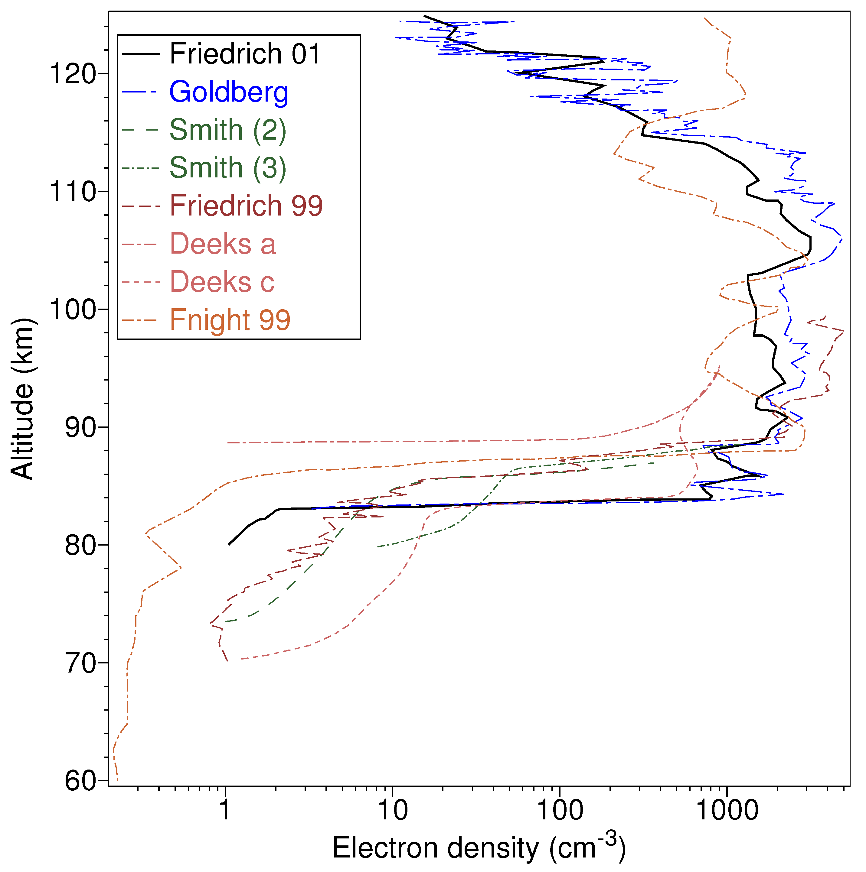
Electron densities deduced from reflection of radio waves at night showed a very sharp decline with altitude at heights 83 and 89 km [1], shown in Figure 1 for summer at sunspot maximum (“Deeks a”) and winter at sunspot minimum (“Deeks c”). Direct measurements of the electron densities using rockets [2] showed similar declines (although not as sharp) at about 87 km (“Smith (2)” and “Smith (3)” in Figure 1). The sharp decline was described as a ledge by Thomas and Harrison [3]. Very sharp ledges were observed in some rocket measurements in the 1990s, with examples reproduced in Figure 1 as “Friedrich 01” [4], “Goldberg” [5], “Friedrich 99” and “Fnight 99” [6].

Nearly simultaneous measurements of O-atom and electron densities [7] showed similarities, including ledges at about 85 km. A simultaneous measurement of electron density and O-atoms [8] showed a ledge in each at about 86 km, with the comment “The pronounced ledge in the electron densities can be reproduced in theoretical models by a similar ledge in atomic oxygen, but sufficient concurrent measurements of the two parameters are not available to prove such an assertion”.

In the Earth’s nighttime mesosphere ionization is produced by cosmic rays and by Lyman-$\alpha$ radiation [9] scattered from the Earth’s geocorona [10]. Sample calculated values of the nighttime electron density from various theories are shown in Figure 2, with the “Fnight 99” measurements included for comparison.

In 1968, Radicella [11] derived a model of the mid-latitude nighttime mesosphere in which atmospheric constituents and reactions were adjusted to reproduce the ledge that was apparent in the measurements by Deeks [1]. Free electrons were assumed to be produced in ionization produced by cosmic rays and precipitating electrons, while Lyman-$\alpha$ was dismissed as an insignificant source. Electrons produced by galactic cosmic rays (GCRs) were presented as equivalent to “ion-pair” production. It was assumed that the free electrons are rapidly attached to molecules to form negative ions, primarily by

$${\mathrm{O}}_2+{\mathrm{O}}_2+e⟶{\mathrm{O}}_2^{-}+{\mathrm{O}}_2$$

and are released by

$$\mathrm{O}+{\mathrm{O}}_2^{-}⟶{\mathrm{O}}_3+e.$$

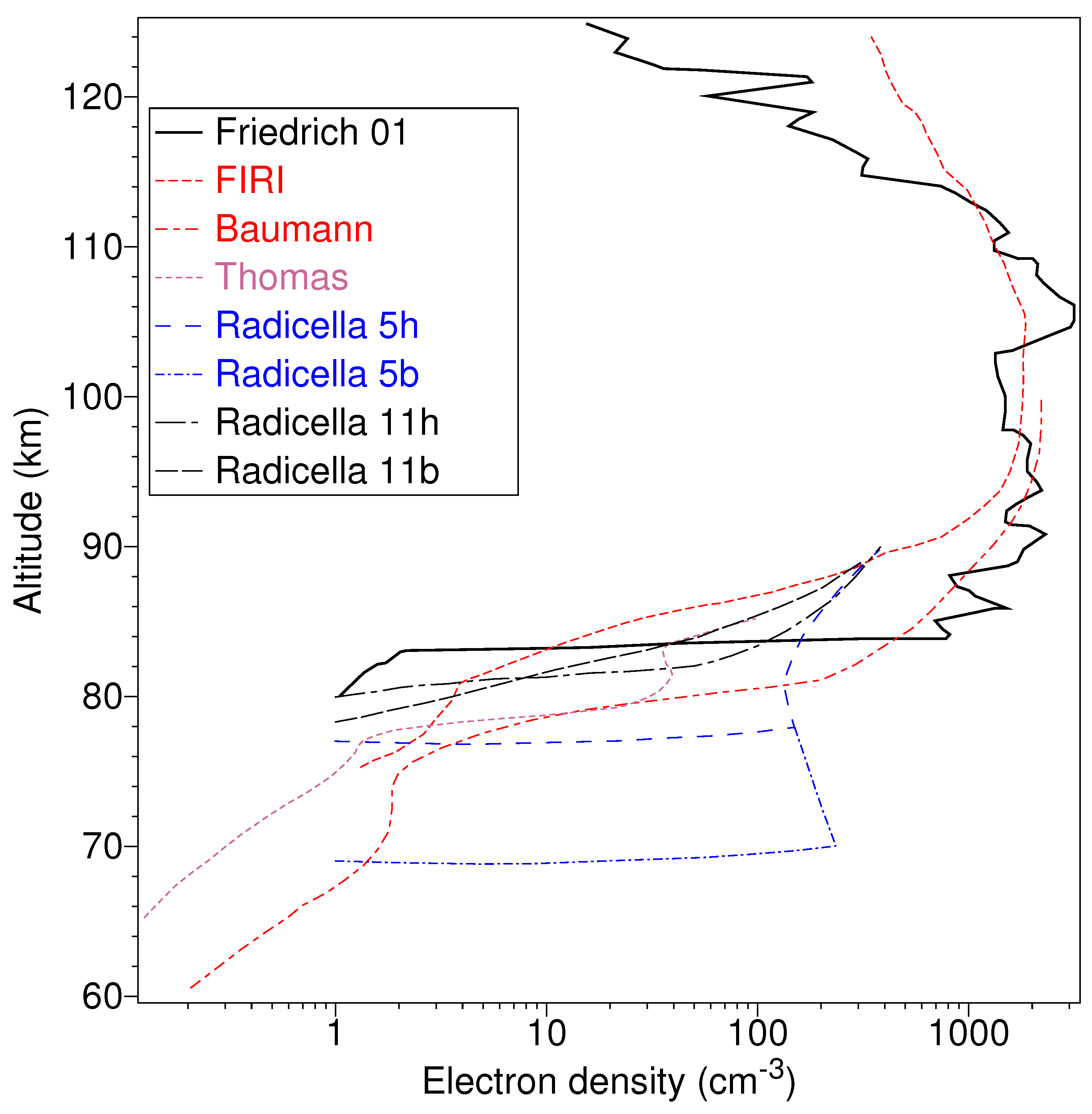
Figure 2. Measured [4] (thick line) and calculated nighttime electron densities as a function of altitude by Friedrich and Torkar [4] (”FIRI”– – –), Baumann et al. [12] (— - —), Thomas and Bowman [13] (- - -) and Radicella [11] (as labelled).

Figure 2. Measured [4] (thick line) and calculated nighttime electron densities as a function of altitude by Friedrich and Torkar [4] (”FIRI”– – –), Baumann et al. [12] (— - —), Thomas and Bowman [13] (- - -) and Radicella [11] (as labelled).

The O${}_2^{-}$ ions start a complex chain of negative-ion reactions, with negative charge finally being removed by ion-ion and electron-ion dissociative recombination. Very sharp electron-density ledges were deduced (“Radicella 5h” and “Radicella5b” in Figure 2), but at heights that were too low. (The plotted curves were nonphysical, having two different densities at the same height.) Less sharp ledges closer to the height in the experimental data (“Radicella 11h” and “Radicella 11b” in Figure 2) were produced by including the reaction

$${\mathrm{N}}_2+{\mathrm{O}}_3^{-}⟶{\mathrm{NO}}_2^{-}+\mathrm{NO}.$$

After Strobel et al. [10] determined that Lyman-$\alpha$ and Lyman-$\beta$ radiation were sufficient to produce observed electron densities in the mesosphere, Thomas et al. [13] assumed free electrons were produced by this and by the same GCR model as used by Radicella [11]. Their model included many more reactions (than Radicella’s) and produced a sharp decline in electron density downward from 79 km (curve “Thomas” in Figure 2). A semiempirical model “FIRI” [4] did not predict the ledge.

Using the Sodankylä Ion and Neutral Chemistry (SIC) model [14], which combines the ion chemistry of the D region with the chemistry of neutral species [15], Baumann et al. [12] added meteor smoke particles, giving the “Baumann” curve in Figure 2. This model gives good agreement with the measured electron densities in the altitude range 80–100 km.

It can be seen in Figure 2 that in all models, the very sharp density gradient in the measurements is not predicted. The slope of the ledge in the recent “Baumann” model is the same as in the much earlier “Thomas” model.

The approach in this paper is to investigate whether the sharp ledge can be predicted by considering the detailed energy-dependent processes of electrons that are produced by Lyman-$\alpha$ radiation. In ionospheric calculations, the rate constants for electron interactions are usually defined as a function of electron temperature $T_e$, based on the assumption that the electron distribution is a Maxwell–Boltzmann distribution. In this work, the electron distribution is calculated as a function of the production and loss mechanisms for electrons, in conjunction with the photochemical model of the chemical reactions. This calculation is facilitated by the method defined and verified by Campbell et al. [16], in which subranges of the electron energy spectrum are treated as chemical species, allowing the electron interactions to be entered as a series of extra rate equations into existing chemical models. As elastic collisions between electrons normally dominate the emergence of a Maxwell–Boltzmann distribution, this method is only applicable where the electron density is very low compared to the molecular density, so that electron–molecule interactions determine the electron energies.

The method is to run simulations of a minimal model, either with electrons assumed to be at the ambient (neutral) temperature, or with electrons initially having a higher temperature. In the latter case the electrons lose energy in small steps in elastic collisions with molecules and larger steps in inelastic collisions producing vibrational excitation of molecules. Thus, the processes of attachment and recombination, which have rate constants that depend on the electron temperature, may proceed at different rates to those for electrons at the neutral temperature, thus giving a different predicted electron density. In all cases, the approach is to perform a semi-implicit time-step simulation [17] of the populations of the chemical species as a function of time.

2. Materials and Methods

Simulations of atmospheric chemical processes usually involve the processing of a set of reactions specified in the form:

$$\mathrm{A}+\mathrm{B}\stackrel{k}{\to }\mathrm{C}+\mathrm{D}+\dots ,$$

(R1)

where A, B, C and D represent atoms or molecules and k is the rate constant. The rate r at which A and B interact is given by:

$$r = k\left[\mathrm{A}\right]\left[\mathrm{B}\right],$$

(1)

where $\left[x\right]$ represents the density of species x and the rate constant k has the units l${}^3$s${}^{-1}$ where “l” is the unit of length in which the density is specified (e.g., cm${}^3$s${}^{-1}$).

A minimal model involving just Lyman-$\alpha$ ionization, recombination with NO${}^{+}$, attachment to O${}_2$, charge exchange involving O${}_3$ and associative electronic detachment is implemented by the 7 reactions (Reaction (R2) [18]; Reactions (R3)–(R8) [13]):

$$\begin{array}{cc}\hfill \mathrm{NO}+\gamma \stackrel{k_{\mathrm{Ly}}}{⟶}{\mathrm{NO}}^{+}+e^{-}& k_{\mathrm{Ly}}=1.24\times {10}^{-18}{\mathrm{cm}}^3{\mathrm{s}}^{-1}\end{array}$$

(R2)

$$\begin{array}{cc}\hfill {\mathrm{NO}}^{+}+e^{-}\stackrel{k_{\mathrm{Rc}}}{⟶}\mathrm{N}+\mathrm{O}& k_{\mathrm{Rc}}=6.0\times {10}^{-7}{\mathrm{cm}}^3{\mathrm{s}}^{-1}\end{array}$$

(R3)

$$\begin{array}{cc}\hfill {\mathrm{O}}_2+{\mathrm{O}}_2+e^{-}\stackrel{k_{{\mathrm{aO}}_2}}{⟶}{\mathrm{O}}_2^{-}+{\mathrm{O}}_2& k_{{\mathrm{aO}}_2}=4.0\times {10}^{-30}{e}^{-193/T{}_n}{\mathrm{cm}}^6{\mathrm{s}}^{-1}\end{array}$$

(R4)

$$\begin{array}{cc}\hfill {\mathrm{O}}_2+{\mathrm{N}}_2+e^{-}\stackrel{k_{{\mathrm{aN}}_2}}{⟶}{\mathrm{O}}_2^{-}+{\mathrm{N}}_2& k_{{\mathrm{aN}}_2}=1.0\times {10}^{-31}{\mathrm{cm}}^6{\mathrm{s}}^{-1}\end{array}$$

(R5)

$$\begin{array}{cc}\hfill {\mathrm{O}}_3+{\mathrm{O}}_2^{-}\stackrel{k_{\mathrm{ce}}}{⟶}{\mathrm{O}}_3^{-}+{\mathrm{O}}_2& k_{\mathrm{ce}}=6.0\times {10}^{-10}{\mathrm{cm}}^3{\mathrm{s}}^{-1}\end{array}$$

(R6)

$$\begin{array}{cc}\hfill {\mathrm{O}}_3^{-}+\mathrm{O}\stackrel{k_{\mathrm{ed}1}}{⟶}{e}^{-}+{\mathrm{O}}_2+{\mathrm{O}}_2& k_{\mathrm{ed}1}=1.0\times {10}^{-10}{\mathrm{cm}}^3{\mathrm{s}}^{-1}\end{array}$$

(R7)

$$\begin{array}{cc}\hfill \mathrm{O}+{\mathrm{O}}_2^{-}\stackrel{k_{\mathrm{ed}2}}{⟶}{\mathrm{O}}_3+e^{-}& k_{\mathrm{ed}2}=1.5\times {10}^{-10}{\mathrm{cm}}^3{\mathrm{s}}^{-1}\end{array}$$

(R8)

The rate constants in (R3)–(R5) are for a Maxwellian distribution of electrons with temperature $T_e$, which for the lower mesosphere is assumed to be equal to the neutral temperature $T_n$. Hereafter, this will be referred to as the “nT” model.

As an example, consider only Reactions (R2) and (R3) for altitude 85 km where [NO] = $2.02\times {10}^6$ cm${}^3$ and the Lyman-$\alpha$ flux $F_{\mathrm{Ly}}$ is as specified by Thomas and Bowman [13]. (Reactions (R4)–(R8) are only significant at lower altitudes.) An equilibrium calculation, where the gain is set equal to the loss rate, gives the electron density as:

$$\left[e^{-}\right] = \sqrt{\frac{F_{\mathrm{Ly}}\left[\mathrm{NO}\right]k_{\mathrm{Ly}}}{k_{\mathrm{Rc}}}} = 79{\mathrm{cm}}^{-3}.$$

(2)

This is consistent with the values of ∼100 cm${}^{-3}$ of Thomas and Bowman [13], allowing for an extra 25% from cosmic rays in their model.

As the electron density is low, the recombination rate will be low and so it will take time for the electron density to reach an equilibrium value in response to a change in input parameters, particularly the Lyman-$\alpha$ ionization rate. Thus, a nonequilibrium calculation is required. A way to simulate the evolution of a set of interacting species is to apply Equation (1) to each Reaction (R1) for a time-step $\Delta t$, so that the change in each species is:

$$-\Delta \left[\mathrm{A}\right] = -\Delta \left[\mathrm{B}\right] = \Delta \left[\mathrm{C}\right] = \Delta \left[\mathrm{D}\right] = k\left[\mathrm{A}\right]\left[\mathrm{B}\right]\Delta t.$$

(3)

For each species i, the gains and losses are added up to give the total gain $G_i$ and total loss $L_i$ so the new density $n_i$ of species i after time $\Delta t$ is:

$$n_i(t+\Delta t) = n_i\left(t\right)+G_i-L_i.$$

(4)

The development of the densities of all species can be simulated by iterative application of Equation (4) over the required time, but the size of $\Delta t$ is limited by the requirement that the density must not go negative and so this “explicit” formula is unsuitable for simulation of systems over long time intervals. This problem is solved in an alternative “semi-implicit” method [17], as detailed by Campbell et al. [16], that transforms Equation (4) to:

$$n_i(t+\Delta t) = \frac{n_i\left(t\right)+G_i}{1+\frac{L_i}{n_i\left(t\right)}}.$$

(5)

To allow the simulation to run to equilibrium with minimum computation time, an adaptive time step $\Delta t$ is required to implement Equation (5) efficiently. The initial value of $\Delta t$ is set very small (${10}^{-8}$ s) and is then successively increased as:

$$\Delta t_{j+1} = f\Delta t_{\min } = fmin\left[\frac{n_i\left(t\right)}{|L_i-G_i|}\mathrm{for}{n}_i\left(t\right)>0\right]\Delta t_j,$$

(6)

where $\Delta t_{\min }$ is the minimum time interval for the density of any of the constituents i to fall to zero in the next time step $\Delta t_{j+1}$ at the current rate of change and $f = 0.0001$ is a factor that acts to reduce the cumulative error in the calculations.

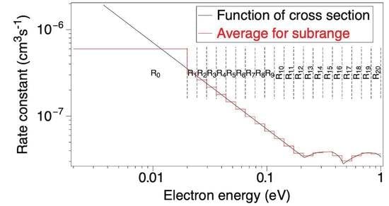
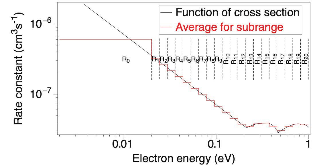
To incorporate energy-dependent electron interactions into a time-step simulation, the method [16] is to split the electron energy range $[E_{\min },E_{\max }]$ into N subranges R${}_1$–R${}_N$, with R${}_0$ set as the range $[0,E_{\min }]$. All electrons within subrange R${}_n$ are assigned the energy E${}_n$, where this is the energy at the midpoint of the subrange.

In place of a single reaction $\mathrm{A}+e\stackrel{k}{⟶}{\mathrm{A}}^{*}+e^{*}$, where A${}^{*}$ represents an excited or ionized state of A and $e^{*}$ a change in energy of the electron, a series of reactions:

$$\mathrm{A}+{\mathrm{R}}_n\stackrel{k_{nm}}{⟶}{\mathrm{A}}^{*}+{\mathrm{R}}_m$$

(R9)

is entered into the list of chemical reactions, with the number density of electrons in each energy range R${}_n$ treated in the same way as the density of a chemical species. (For example, in the current implementation the number of electrons in the range [0, $E_{\min }$] is stored in a variable R₀, analogous to the number of N${}_2$ molecules being stored in a variable N₂.)

A model (designated “EI”) that includes the detailed electron interactions has the reactions above modified to:

$$\begin{array}{c}\hfill \mathrm{NO}+\gamma \stackrel{k_{\mathrm{Ly}}}{⟶}{\mathrm{NO}}^{+}+{\mathrm{R}}_{n_{\mathrm{Ly}}}\end{array}$$

(R10)

$$\begin{array}{c}\hfill {\mathrm{NO}}^{+}+{\mathrm{R}}_n\stackrel{k_{\mathrm{Rc}}^n}{⟶}\mathrm{N}+\mathrm{O}\end{array}$$

(R11)

$$\begin{array}{c}\hfill {\mathrm{O}}_2+{\mathrm{O}}_2+{\mathrm{R}}_n\stackrel{k_{{\mathrm{O}}_2}^n}{⟶}{\mathrm{O}}_2^{-}+{\mathrm{O}}_2\end{array}$$

(R12)

$$\begin{array}{c}\hfill {\mathrm{O}}_2+{\mathrm{N}}_2+{\mathrm{R}}_n\stackrel{k_{{\mathrm{N}}_2}^n}{⟶}{\mathrm{O}}_2^{-}+{\mathrm{N}}_2\end{array}$$

(R13)

$$\begin{array}{c}\hfill {\mathrm{O}}_3+{\mathrm{O}}_2^{-}\stackrel{k_{\mathrm{ce}}}{⟶}{\mathrm{O}}_3^{-}+{\mathrm{O}}_2\end{array}$$

(R14)

$$\begin{array}{c}\hfill {\mathrm{O}}_3^{-}+\mathrm{O}\stackrel{k_{\mathrm{ed}1}}{⟶}{\mathrm{R}}_0+{\mathrm{O}}_2+{\mathrm{O}}_2\end{array}$$

(R15)

$$\begin{array}{c}\hfill \mathrm{O}+{\mathrm{O}}_2^{-}\stackrel{k_{\mathrm{ed}2}}{⟶}{\mathrm{O}}_3+{\mathrm{R}}_0\end{array}$$

(R16)

and also includes vibrational excitation of the first level of N${}_2$ and O${}_2$:

$$\begin{array}{c}\hfill {\mathrm{N}}_2(\nu =0)+{\mathrm{R}}_n\stackrel{k_{{\mathrm{vibN}}_2}^{nm}}{⟶}{\mathrm{N}}_2(\nu =1)+{\mathrm{R}}_m\end{array}$$

(R17)

$$\begin{array}{c}\hfill {\mathrm{O}}_2(\nu =0)+{\mathrm{R}}_n\stackrel{k_{{\mathrm{vibO}}_2}^{nm}}{⟶}{\mathrm{O}}_2(\nu =1)+{\mathrm{R}}_m\end{array}$$

(R18)

and elastic collisions of electrons with N${}_2$ and O${}_2$:

$$\begin{array}{c}\hfill {\mathrm{N}}_2+{\mathrm{R}}_n\stackrel{k_{{\mathrm{elasN}}_2}^{nm}}{⟶}{\mathrm{N}}_2+{\mathrm{R}}_m(m=n-1)\end{array}$$

(R19)

$$\begin{array}{c}\hfill {\mathrm{O}}_2+{\mathrm{R}}_n\stackrel{k_{{\mathrm{elasO}}_2}^{nm}}{⟶}{\mathrm{O}}_2+{\mathrm{R}}_m(m=n-1).\end{array}$$

(R20)

In the following subsections, the rate constants for recombination ($k_{\mathrm{Rc}}^n$), attachment ($k_{{\mathrm{O}}_2}^n$ and $k_{{\mathrm{N}}_2}^n$), vibrational excitation ($k_{{\mathrm{vibN}}_2}^{nm}$ and $k_{{\mathrm{vibO}}_2}^{nm}$) and elastic collsions ($k_{{\mathrm{elasN}}_2}^{nm}$ and $k_{{\mathrm{elasO}}_2}^{nm}$) are deduced. Due to lack of information about the energy of the electrons released in Reactions (R15) and (R16), it is assumed here that they are at $T_n$ and so are placed in subrange R${}_0$. Lyman-$\alpha$ has an energy of 10.21 eV and NO has an ionization energy of 9.2642 eV, so the electrons produced are assumed to have an energy of 0.944 eV. By setting $E_{\max }$ to 1.0 eV, R${}_{n_{\mathrm{Ly}}}$=R${}_N$.

2.1. NO⁺ Recombination

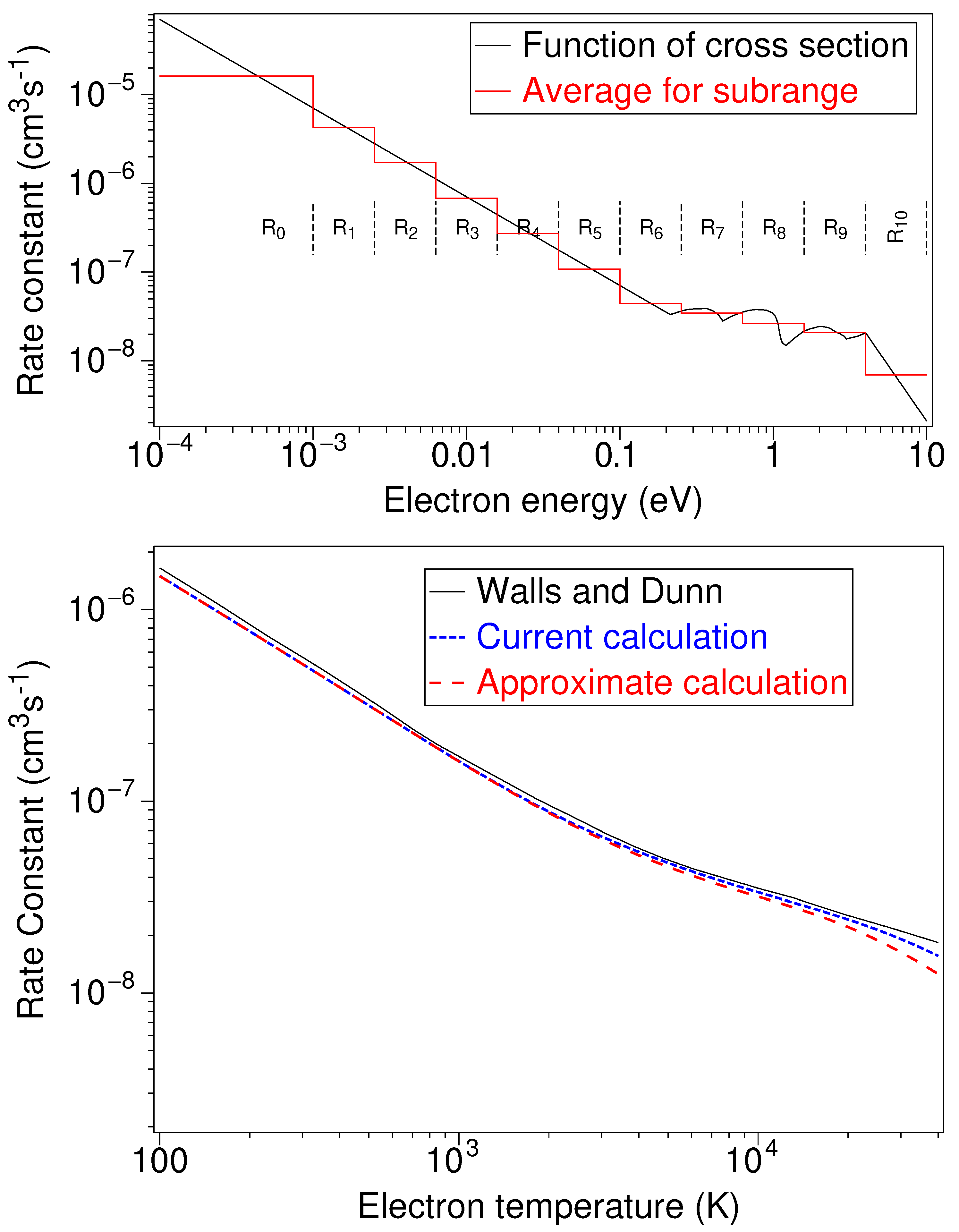
Cross-sections as a function of energy for Reaction (R11) were measured by Walls and Dunn [19]. From these, they calculated rate constants for Maxwellian electron distributions as a function of electron temperature $T_e$, shown by the solid line in the lower panel of Figure 3.

The rate constant $k_{\mathrm{Rc}}$ is related to the cross-section $\sigma$ by:

$$k_{\mathrm{Rc}}\left(E\right)=v\sigma \left(E\right)=\sqrt{\frac{2E}{m_e}}\sigma \left(E\right)$$

(7)

where v is the speed of the electron, $m_e$ is the electron mass and $\sigma \left(E\right)$ is the cross section for electrons of energy E. Applying this to the measured cross sections (digitised from a graph of Walls and Dunn) gives the curve in the upper panel of Figure 3.

To calculate the rate constant for a Maxwellian distribution, an integration is made of the product of $k_{\mathrm{Rc}}\left(E\right)E$ and the Electron Energy Distribution Function $F\left(E\right)$ at each energy E. These calculations are repeated here to verify the current implementation, giving the dashed curve in Figure 3. These values are slightly less than those of Walls and Dunn, but this discrepancy could be due to inaccuracy in the original publication and/or digitisation errors.

To demonstrate the application of the set of Reaction (R9) and investigate the accuracy of the approximation, the electron energy range $0.0001–10$ eV is divided into 11 subranges R${}_0$–R${}_{10}$ and the rate constants are averaged in each subrange (as shown by the horizontal segments in the upper panel of Figure 3). The rate constants for Maxwellian distributions at each temperature $T_e$ are calculated by applying the 11 average rate constants to the Maxwellian electron density functions at the centre of each subrange:

$$k_{\mathrm{Rc}}\left(T_e\right)={\sum }_{n=0}^{10}{k}_{\mathrm{Rc}}^{n}F\left(E_n\right)(E_{n,n+1}-E_{n-1,n})$$

(8)

where $E_{n,n+1}$ is the energy at the boundary of subranges R${}_n$ and R${}_{n+1}$. Plotting the rate constants calculated using Equation (8) in the lower panel of Figure 3 shows that there is little difference between the precise values and the approximation, showing that the representation of the electron spectrum by just 11 average values is a viable approach.

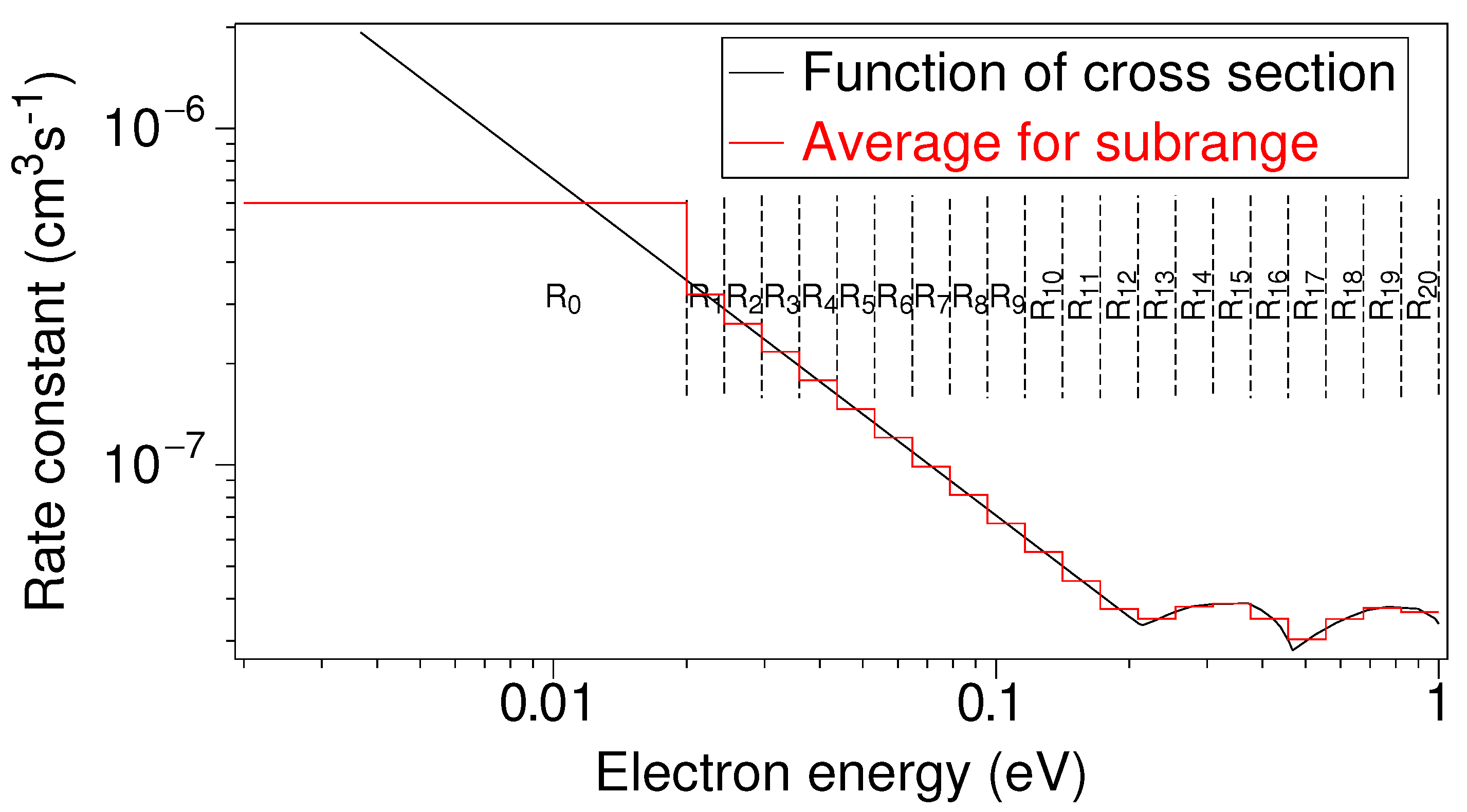
For the application here $[E_{\min },E_{\max }] \mathrm{is} \mathrm{set} \mathrm{to} [0.02,1.0]$, so that the 0.944-eV electrons produced by Lyman-$\alpha$ ionization are in the highest-energy subrange and the electron energy of 0.019 eV, corresponding to the neutral temperature of 220 K, is in the lowest subrange R${}_0$. As shown in Figure 4 R${}_0$ is defined as the range [0.002–0.02], for which the averaged value of the rate constant is $6.0\times {10}^{-7}$. This is the value used by Thomas and Bowman [13] in the study that is to be partially emulated here. In this case, 21 energy subranges are used to be consistent with the resolution needed for vibrational excitation (to be described below).

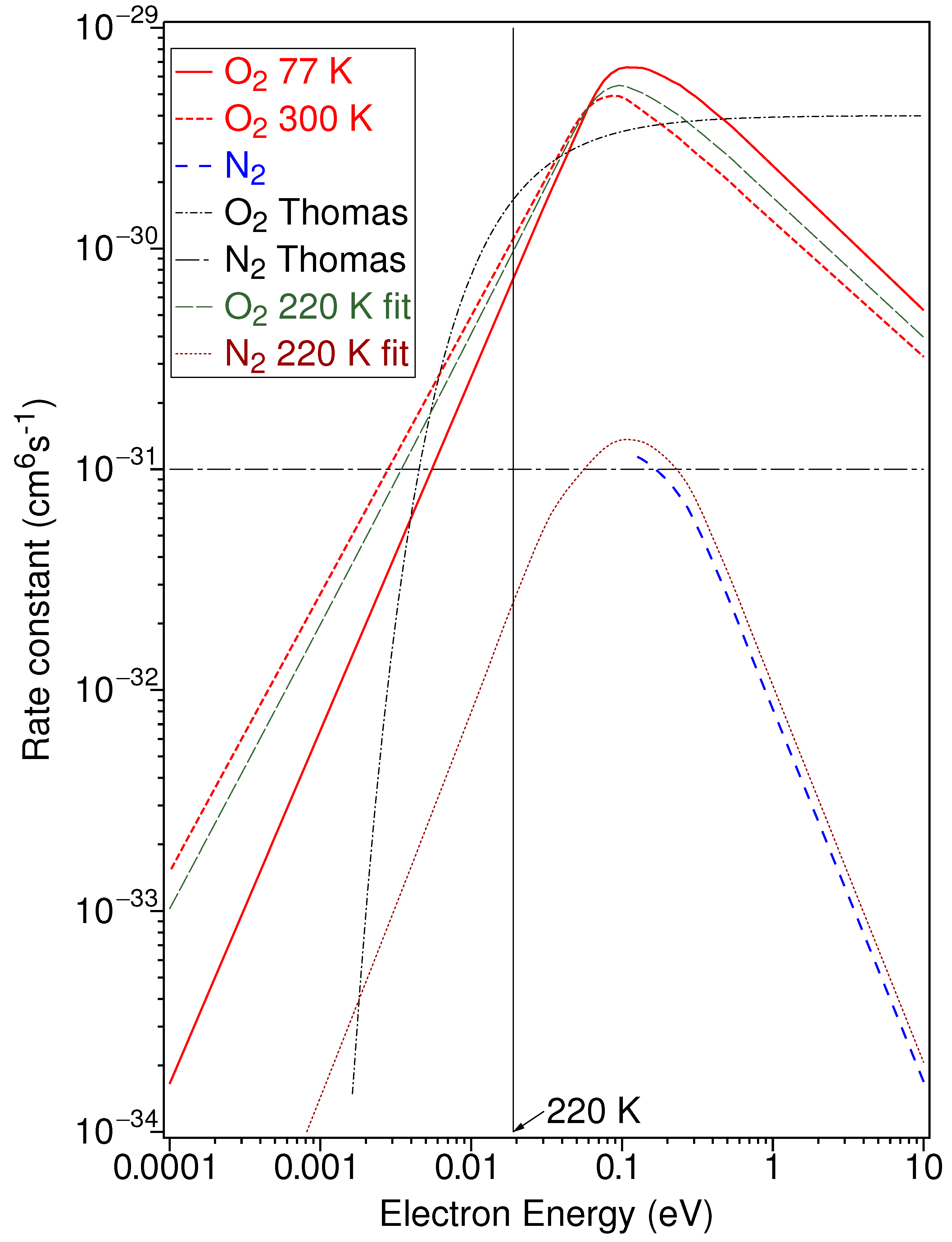
2.2. Attachment

Measured rate constants for attachment of electrons for O${}_2$ as a function of electron energy [20] are reproduced in Figure 5 for Reaction (R12) at neutral temperatures of 77 K and 300 K and for Reaction (R13) at 300 K. For comparison, the rate constants for these reactions for a Maxwellian distribution of electrons as a function of the electron temperature are shown. A vertical line corresponding to the neutral temperature of 220 K shows that the rate constants for electrons at ∼0.1 eV are substantially higher than that used in the nT model (labelled “O${}_2$ Thomas”) for Reaction (R12), i.e., about $2\times {10}^{-30}$ cm${}^6$s${}^{-1}$ at T${}_n = 220$ K.

To obtain the rate constants for Reaction (R12) at any neutral temperature, an interpolation is performed between the values at 77 K and 300 K. The shape of the curve at 300 K is copied to extend the measured values for Reaction (R13) down through lower energies, then the entire curve is mapped to another neutral temperature by comparison with the interpolation for Reaction (R12). The results of these operations are plotted in Figure 5 for a neutral temperature of 220 K. (i.e., “O${}_2$ 220 K fit” and “N${}_2$ 220 K fit”).

To obtain the rate coefficients $k_{{\mathrm{O}}_2}^n$ and $k_{{\mathrm{N}}_2}^n$, the functions plotted are then averaged over subranges in the same way as for the recombination rate constants.

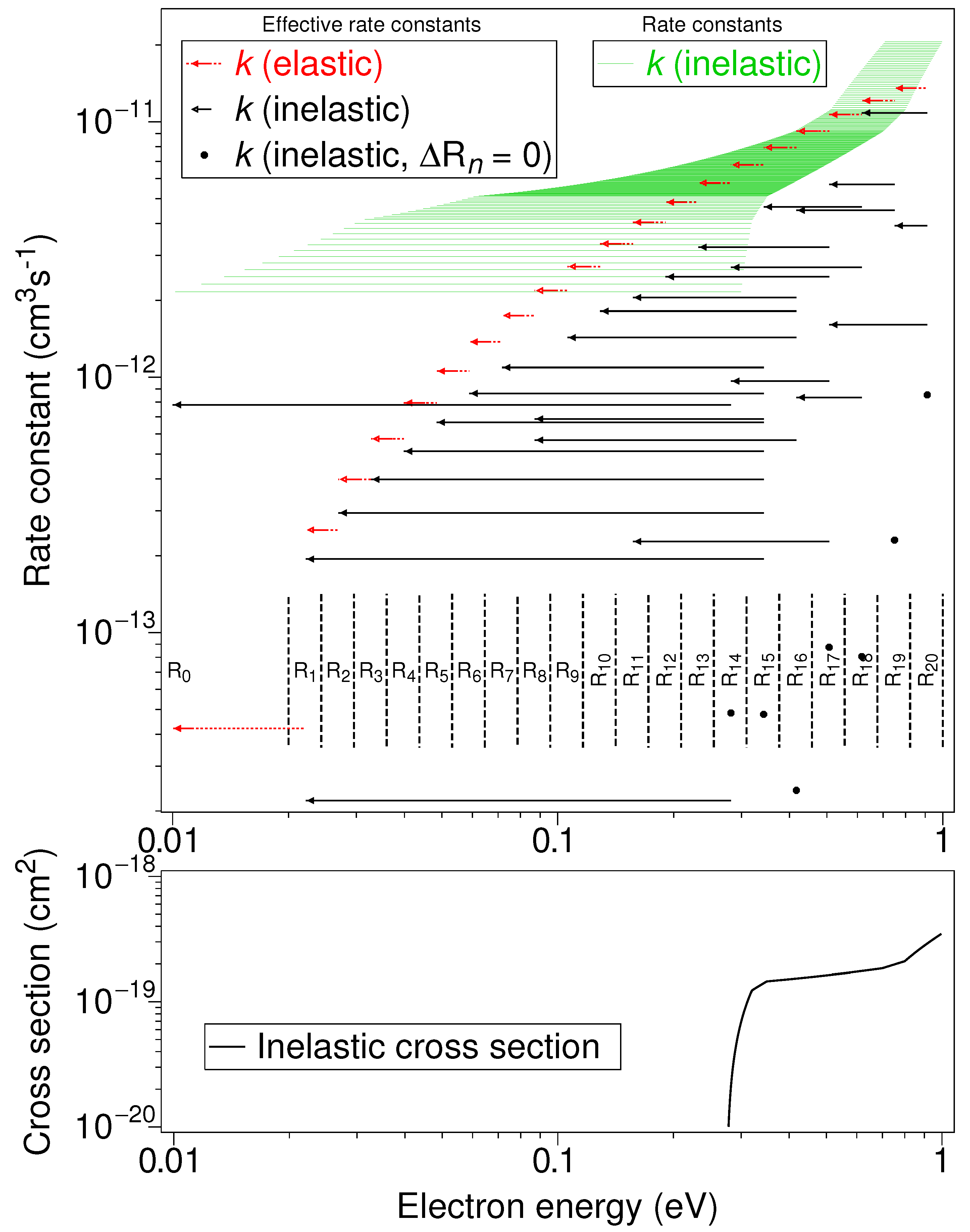
2.3. Vibrational Excitation and Elastic Collisions

The 0.944-eV electrons produced in Reaction (R10) can excite the first vibrational of N${}_2$, losing 0.289 eV in the process. The inelastic cross sections ${\sigma }_{01}\left(E\right)$ for this excitation (the “Flinders” set of Campbell et al. [21]) are shown as a function of electron-impact energy in the lower panel of Figure 6. Representative rate constants $k_{{\mathrm{vibN}}_2}\left(E\right)$, calculated using Equation (7), are shown by lines drawn from the initial energy of the electron to the final energy, at the level of the rate constant on the vertical axis in the upper panel.

The averaged rate constants for all transitions from one electron-energy subrange to another are shown by arrows (with solid lines) drawn from the centre of the initial subrange to the centre of the final subrange. These arrows represent the set of Reaction (R17). (The bullets show minor adjustments, where the electron remains in the same subrange, to implement energy conservation for logarithmically-spaced energy intervals [16].) For vibrational excitation of O${}_2$, the cross-sections published by Jones et al. [22] were used to derive the averaged rate constants for Reaction (R18).

The average energy transferred in an elastic collision between an electron with energy E and a molecule of mass M is given by [23]

$$\Delta E = 2\frac{m_e}{M}{\sigma }_{\mathrm{MT}}\left(E\right)Ev$$

(9)

where ${\sigma }_{\mathrm{MT}}$ is the elastic momentum transfer cross-section. These cross-sections were obtained from Table 6.3.5.3 for e–N${}_2$ collisions and Table 6.3.5.6 for e–O${}_2$ collisions in a compilation by Elford et al. [24].

The rate constant for elastic transitions of electrons from subrange m to $m-1$ is then that required to transfer energy $E_m-E_{m-1}$ i.e.,:

$$k_{\mathrm{elas}}^{m,m-1} = \frac{\Delta E}{E_m-E_{m-1}}.$$

(10)

These averaged rate constants are shown by the arrows with dotted lines in Figure 6.

2.4. Emissions Arising from Vibrational Excitation

Emissions can arise from vibrationally excited O${}_2$ and N${}_2$, by Reactions (R21)–(R23) [25] and (R24) [26]:

$${\mathrm{N}}_2\left(1\right)+\mathrm{O}\stackrel{k_{\mathrm{r}1}}{⟶}{\mathrm{N}}_2\left(0\right)+\mathrm{O}+2331{\mathrm{cm}}^{-1}{k}_{\mathrm{r}1}=2.45\times {10}^{-22}{T}^{2.87}$$

(R21)

$${\mathrm{O}}_2\left(1\right)+{\mathrm{N}}_2\stackrel{k_{\mathrm{r}2}}{⟶}{\mathrm{O}}_2\left(0\right)+{\mathrm{N}}_2+1556{\mathrm{cm}}^{-1}{k}_{\mathrm{r}2}=1.364\times {10}^{-12}T{e}^{-137.93/T^{1/3}}$$

(R22)

$${\mathrm{O}}_2\left(1\right)+{\mathrm{O}}_2\stackrel{k_{\mathrm{r}3}}{⟶}{\mathrm{O}}_2+{\mathrm{O}}_2+1556{\mathrm{cm}}^{-1}{k}_{\mathrm{r}3}=1.364\times {10}^{-12}T{e}^{-137.93/T^{1/3}}$$

(R23)

$${\mathrm{N}}_2\left(1\right)+{\mathrm{CO}}_2\left(0\right)\stackrel{k_{\mathrm{r}4}}{⟶}{\mathrm{N}}_2\left(0\right)+{\mathrm{CO}}_2\left({\nu }_3\right)k_{\mathrm{r}4}=8.91\times {10}^{-12}{T}^{-1}$$

(R24)

In the last case, the excited CO${}_2$ can produce 4.3 μm radiation [26] and also emissions at 2.7 μm, 2.0 μm, etc. [25].

3. Results

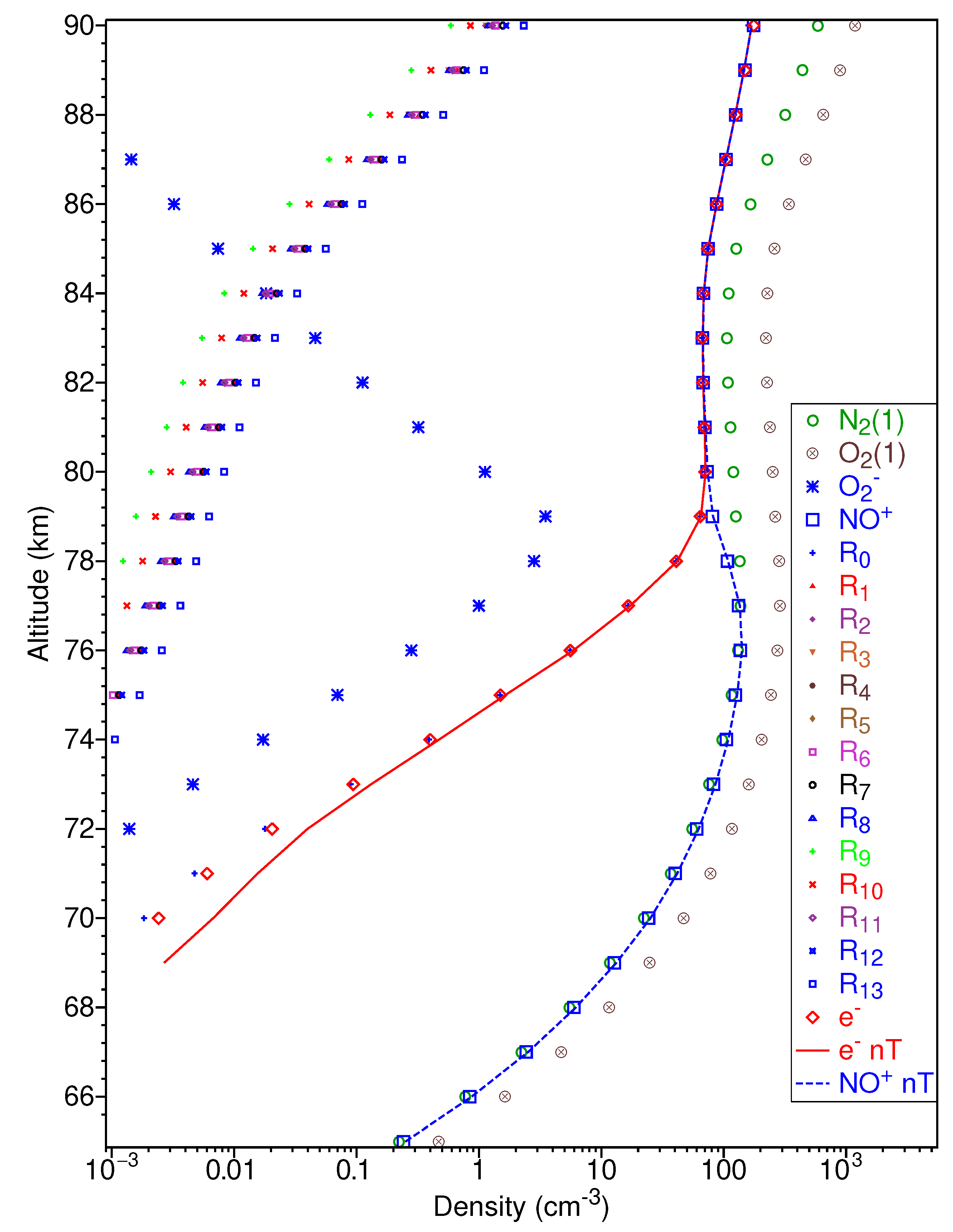
In Figure 7, the “nT” model (Reactions (R2)–(R8)) is applied with rate constants based on a Maxwellian distribution of electrons at a neutral temperature $T_n =$ 220 K. The electron density as a function of altitude (shown by the solid red line, labelled “e${}^{-}$ nT”) is calculated by time-step simulation applied for midnight conditions for a time of 10 h, starting with zero electron density.

The simulation is then repeated for the electron interaction model without elastic scattering i.e., Reactions (R10)–(R18), with the densities after 10 h shown by symbols. At 77 km and below the electron density is less than in the “nT” model, and substantially less at 72 km and below. Most of the electrons are in subrange R${}_0$, but some are in subranges R${}_1$–R${}_{13}$, with the proportion increasing with altitude. Densities of vibrationally excited molecules N${}_2$(1) and O${}_2$(1) are higher than the electron densities.

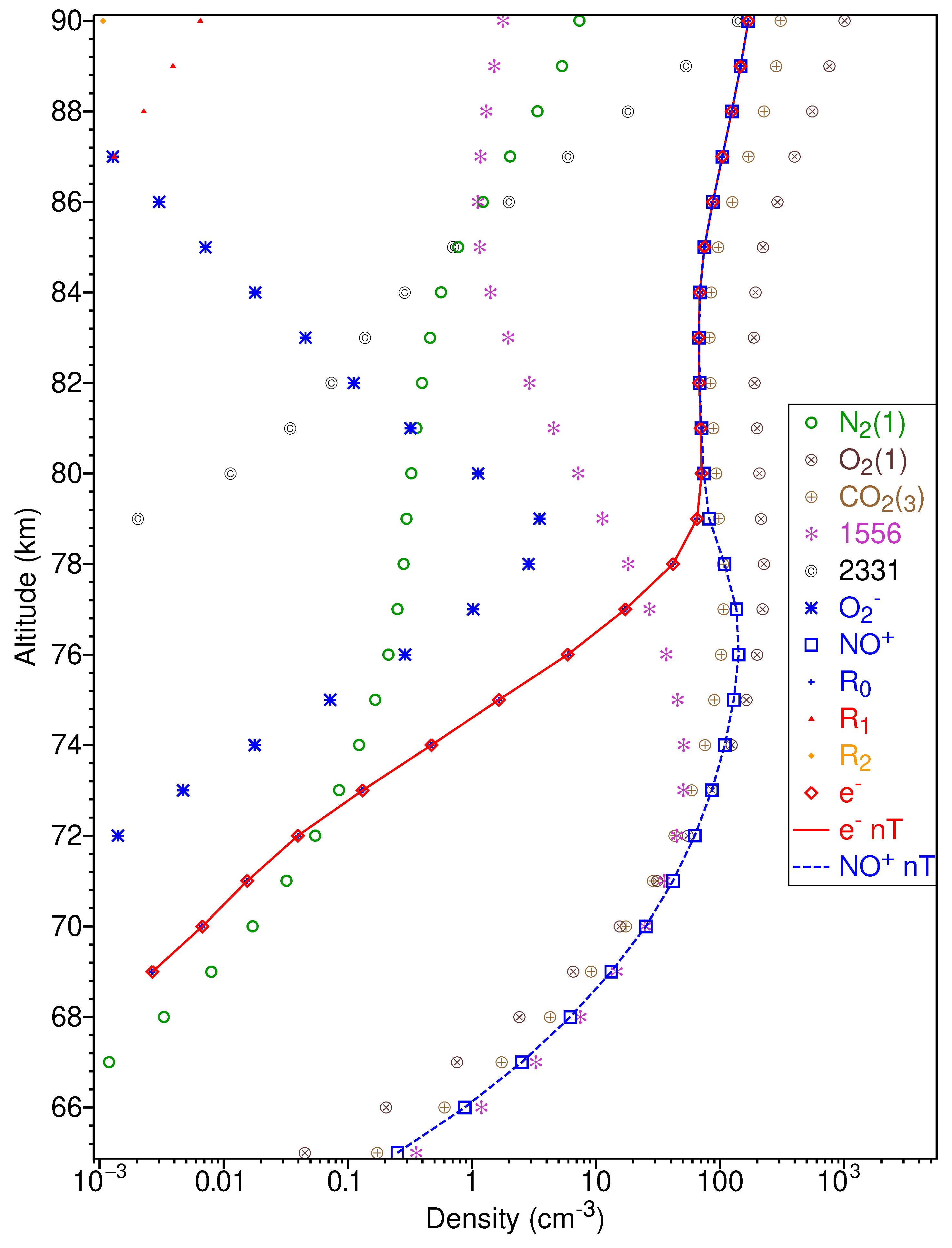
The “EI” model is repeated in Figure 8 with elastic scattering (Reactions (R19) and (R20)) and emission-producing Reactions (R21)–(R24) included. There is now no apparent difference in the electron densities for the “nT” and “EI” cases. Here (for the same density range as before), there are electrons in subranges R${}_1$ and R${}_2$ only at the highest altitudes, with all in R${}_0$ at lower altitudes. The total production of CO${}_2\left({\nu }_3\right)$ (labelled “CO${}_2{(}_3)$”) is plotted as a density, as are the number of photons/cc emitted in 10 h for 2331 cm${}^{-1}$ and 1556 cm${}^{-1}$.

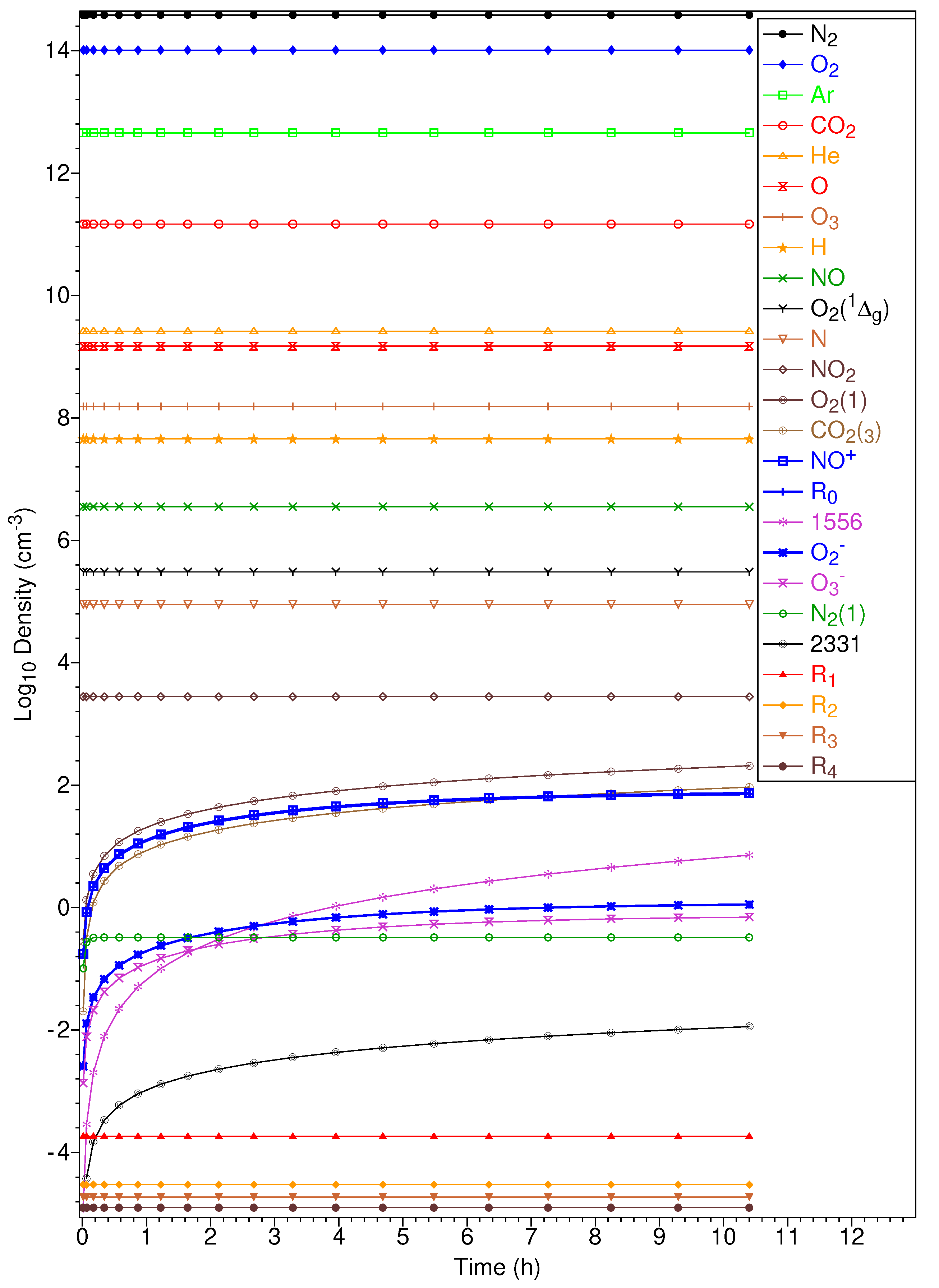
In Figure 9, the densities of both background species and those produced by the EI model are shown as a function of time, at an altitude of 80 km. The electron density reaches the equilibrium value of ∼80 cm${}^{-3}$ after about 6 h.

4. Discussion

In Figure 7, there is little difference between the electron densities calculated by the nT and EI models, except for a reduction at altitudes 71–76 km. The reduction is as expected due to the higher rate of the Reaction (R12) at higher electron temperatures. However, as the reduction is small, it does not provide an explanation for the D-region ledge. This is more evident in Figure 8 when the electrons also lose energy in elastic collisions with N${}_2$ and O${}_2$, with the result that there is no discernible difference in the predicted electron densities. In the nT model, the electrons do not have sufficient energy to produce vibrational excitation of molecules, but, as seen in Figure 8, there is some production of vibrationally excited N${}_2$(1) and O${}_2$(1), leading to radiative emissions at 1556 cm${}^{-1}$ and 2331 cm${}^{-1}$ and from CO${}_2\left({\nu }_3\right)$. However, these emissions may be very small compared to what is expected due to thermal production. For example, if the gas is at thermal equilibrium, at 80 km [N${}_2$] = $3.8\times {10}^{14}$ cm${}^{-3}$, so [N${}_2$(1)] is expected to be about $9\times {10}^7$ cm${}^{-3}$, which is much larger than the predicted density of ∼0.3 cm${}^{-3}$. However, this depends on the rate of translational–vibrational (TV) transitions, which would need to be included in the model to make an accurate prediction of the thermal emissions.

In Figure 9, it is shown that it takes about 6 h for the electron density to reach the equilibrium value. While starting from zero electron density is not physically realistic, it implies that there will be a substantial time lag in the reduction in electron density from daytime values, compared to instantaneous equilibrium. Thus time-dependent modelling is required for calculations of the nighttime mesosphere. This suggests that it could be worthwhile to implement the above calculation (which applied midnight parameters over 10 h) to a fully time-dependent simulation, with the Lyman-$\alpha$ flux varied according to time of day or night. As this flux and also the rates of chemical reactions vary with altitude, it is likely that the rate of progress towards equilibrium will also vary with height, producing a different altitude profile for the electron density relative to that produced by assuming equilibrium is attained.

The loss of energy by higher-energy electrons due to elastic collisions with thermal electrons is not included in this study. While it is not expected to be significant, given the very high ratio of molecules to electrons, it does need to be quantified so that the method can be applied with confidence at higher electron densities.

The EI approach could be useful in predicting emissions produced by higher-energy electrons (>5 eV) that could not be produced by thermal excitation. This depends on the secondary electron spectrum produced by cosmic rays—in particular whether cosmic rays produce ions and electrons with high energy, or ion-pairs from which electrons are then released with low energy. Thus, the EI model could be used to predict emissions that could be used as diagnostics of the secondary electron spectrum produced by cosmic rays.

5. Conclusions

A time-step simulation that includes energy-dependent electron interactions has been applied to simulate electron interactions in the Earth’s quiet nighttime mesosphere. A minimal model with just a few processes (Lyman-$\alpha$ production of electrons and NO${}^{+}$, attachment of electrons to O${}_2$, charge transfer to O${}_3$, associative electron detachment and dissociative recombination of electrons with NO${}^{+}$) was run for both the assumption that the electrons are at the neutral temperature and that they have higher energy for some finite time as they progressively lose it in elastic and inelastic collisions with molecules. It was found that there is little difference in the electron densities predicted by the two approaches, so consideration of energy-dependent reaction rates does not provide an explanation for the D-region ledge. It was found that the presence of higher-energy electrons leads to the production of vibrationally excited N${}_2$ and O${}_2$ with subsequent radiative emissions, but that the densities are small compared to those expected from thermal excitation. However, the EI model could be used to predict emissions produced by cosmic rays, if these produce higher-energy electrons. It was also found that it takes of the order of 6 h for the calculated electron densities to reach equilibrium at 80 km, showing that only time-dependent models are adequate for calculations of the lower mesosphere.