Article

Machine-Learning-Based Downscaling of Hourly ERA5-Land Air Temperature over Mountainous Regions

by
Badr-eddine Sebbar
1,2,*,
Saïd Khabba
1,3,
Olivier Merlin
2,
Vincent Simonneaux
2,
Chouaib El Hachimi
1,
Mohamed Hakim Kharrou
4 and
Abdelghani Chehbouni
1,2,4
1
Center for Remote Sensing Applications, Mohammed VI Polytechnic University (UM6P), Ben Guerir 43150, Morocco
2
Centre d’Etudes Spatiales de la Biosphère (CESBIO), Université de Toulouse, CNES, CNRS, IRD, UPS, 31400 Toulouse, France
3
LMFE, Physics Department, Faculty of Sciences Semlalia, Cadi Ayyad University, Marrakech 40000, Morocco
4
International Water Research Institute (IWRI), Mohammed VI Polytechnic University (UM6P), Ben Guerir 43150, Morocco
*
Author to whom correspondence should be addressed.
Atmosphere 2023, 14(4), 610; https://doi.org/10.3390/atmos14040610
Submission received: 26 January 2023 / Revised: 7 February 2023 / Accepted: 9 February 2023 / Published: 23 March 2023
(This article belongs to the Special Issue Statistical Approaches in Climatic Parameters Prediction)

Abstract

:
In mountainous regions, the scarcity of air temperature (Ta) measurements is a major limitation for hydrological and crop monitoring. An alternative to in situ measurements could be to downscale the reanalysis Ta data provided at high-temporal resolution. However, the relatively coarse spatial resolution of these products (i.e., 9 km for ERA5-Land) is unlikely to be directly representative of actual local Ta patterns. To address this issue, this study presents a new spatial downscaling strategy of hourly ERA5-Land Ta data with a three-step procedure. First, the 9 km resolution ERA5 Ta is corrected at its original resolution by using a reference Ta derived from the elevation of the 9 km resolution grid and an in situ estimate over the area of the hourly Environmental Lapse Rate (ELR). Such a correction of 9 km resolution ERA5 Ta is trained using several machine learning techniques, including Multiple Linear Regression (MLR), Support Vector Regression (SVR), and Extreme Gradient Boosting (Xgboost), as well as ancillary ERA5 data (daily mean, standard deviation, hourly ELR, and grid elevation). Next, the trained correction algorithms are run to correct 9 km resolution ERA5 Ta, and the corrected ERA5 Ta data are used to derive an updated ELR over the area (without using in situ Ta measurements). Third, the updated hourly ELR is used to disaggregate 9 km resolution corrected ERA5 Ta data at the 30-meter resolution of SRTM’s Digital Elevation Model (DEM). The effectiveness of this method is assessed across the northern part of the High Atlas Mountains in central Morocco through (1) k-fold cross-validation against five years (2016 to 2020) of in situ hourly temperature readings and (2) comparison with classical downscaling methods based on a constant ELR. Our results indicate a significant enhancement in the spatial distribution of hourly local Ta. By comparing our model, which included Xgboost, SVR, and MLR, with the constant ELR-based downscaling approach, we were able to decrease the regional root mean square error from approximately 3 C to 1.61 C, 1.75 C, and 1.8 C, reduce the mean bias error from −0.5 C to null, and increase the coefficient of determination from 0.88 to 0.97, 0.96, and 0.96 for Xgboost, SVR, and MLR, respectively.

1. Introduction

Access to spatially and temporally consistent climate data at high spatial and temporal resolutions has progressively turned into a growing need in the 21st century for being paramount to numerous fields of study that investigate ecological, hydrological, and climate change processes, among others [1,2,3,4,5,6,7]. Using numerical weather models and data assimilation techniques to produce model-based reanalysis products is one viable strategy for generating climate datasets in light of this need [8,9,10,11]. Several international and local meteorological centers and data assimilation offices have collaborated over the past few decades to make numerous reanalysis products available to the public [12]. Examples of the most popular reanalysis products are: the ERA5 and ERA5-Land from the European Centre for Medium Range Weather Forecasts (ECMWF); the second version of Modern-Era Retrospective Analysis for Research and Applications (MERRA2) [13] produced by NASA’s Global Modeling and Assimilation Office (GMAO); the second version of Climate Forecast System Reanalysis (CFSv2) from the National Centers for Environment Prediction and National Center for Atmospheric Research (NCEP/NCAR) [14]; NCEP/NCAR Global Reanalysis Products from NCEP and NCAR [15,16]; and the Japanese 55-year Reanalysis (JRA-55) [17] from the Japanese Meteorological Agency (JMA ) [12,18]. The common key strength of the numerous existing reanalysis products resides in providing global datasets devoid of gaps, at high temporal resolution, and over long time periods (generally over three or more decades). Still, reanalysis data frequently fail to simulate many of the processes that drive regional and local climate variability. Their limitations lie in their incapability of accurately depicting sub-km-scale climate variables at the needed timescales and do not allow for proper representations of the local topography and sub-grid-scale features that are essential in areas with complex terrain, microclimates or narrow mountain valleys, as highlighted by Holden et al. [19], Zhang et al. [20], Le Roux et al. [21], Alessi and DeGaetano [22], and Zhang et al. [23]. When evaluated in contrast to observational data, the raw output data are regularly found to have systematic biases [24,25], limiting their usefulness for local applications [26]. There is consequently a need to make local-scale predictions more skillful by utilizing reanalysis data as input. In this context, a variety of techniques, such as downscaling methods, have been developed to bridge the gap between the scale at which data are available and the scale at which they are needed. The commonly used methods include dynamical downscaling and statistical downscaling [27].
Dynamical and statistical downscaling techniques are frequently used to refine coarser climate products to higher resolution [28,29]. The former is a widely used methodology to enhance the spatial information [30], in which a higher-resolution model, such as a regional climate model (RCM), can be driven by reanalysis data and run at spatial resolutions of up to a few meter projections (e.g., [31]), at which complex topography and smaller-scale processes are better represented [32]. This approach can give a very good simulation of local atmospheric conditions; however, it has significant computational cost [30,31,33,34]. Statistical downscaling methods, on the other hand, use statistical relationships to anticipate the evolution of local variables from large-scale variables. They are computationally less demanding and represent a more flexible alternative to dynamical downscaling. These methods have been shown to be effective in reproducing the fine-scale temperature variability over mountainous regions, particularly when using local observations (e.g., [1,35,36]).
This paper focuses on reanalysis air temperature (Ta) disaggregation over complex terrain since (i) it is one of the most important input variables in agro-environmental models and a crucial field for the vast majority of weather and climate applications, including climate change studies (e.g., [37,38]), and (ii) this variable is projected to change significantly in regions with irregular topography, i.e., complex topography of mountain landscapes known to have a highly variable climate, with microclimates that can differ significantly from the surrounding area (e.g., [39,40]). Thus, having high-resolution Ta data over mountains allows for a better understanding of the complex microclimates that exist within mountain ranges and can be particularly useful for predicting weather patterns and for understanding the impacts of climate change on these regions. Several studies describe the spatial interpolation methods used for downscaling in meteorology and climatology [37,41]. These techniques include nearest neighbor methods, splines, regression, kriging, and cokriging but also machine learning techniques such as Artificial Neural Networks and Support Vector Machines [42,43,44,45]. None of these studies, however, focused on adjusting reanalysis data to the regional real measured conditions prior to downscaling, nor worked on the hourly timestep required for hydrological modeling, relying on the availability of quality meteorological inputs at the simulation time step [46]. Recently, Sourp et al. [47] developed a snow reanalysis pipeline using downscaled ERA5 and ERA5-Land data. The downscaling is based on the MicroMet model [48,49], which performs spatial interpolation of meteorological variables using 100 m DEM [47]. Particularly, air temperature is downscaled to an hourly timestep using the DEM and constant monthly Environmental Lapse Rates (ELRs).
Extending these previous ideas, a machine learning/statistical downscaling scheme is designed in this study to disaggregate hourly air temperature data with a 30 m spatial resolution from the 9 km ERA5-Land Ta. The main originality relies on the assumption that the temporal variability of ELR should be taken into account for improving the spatial distribution of downscaled Ta estimates. The approach is tested in a steep-sided catchment in the western part of the High Atlas Mountains in central Morocco, where in situ Ta measurements are available from 2016 to 2020. The paper is organized as follows: the study area, datasets, and the methodology are presented in Section 2. Section 3 presents and discusses the results, while Section 4 outlines the principal conclusions.

2. Materials and Methods
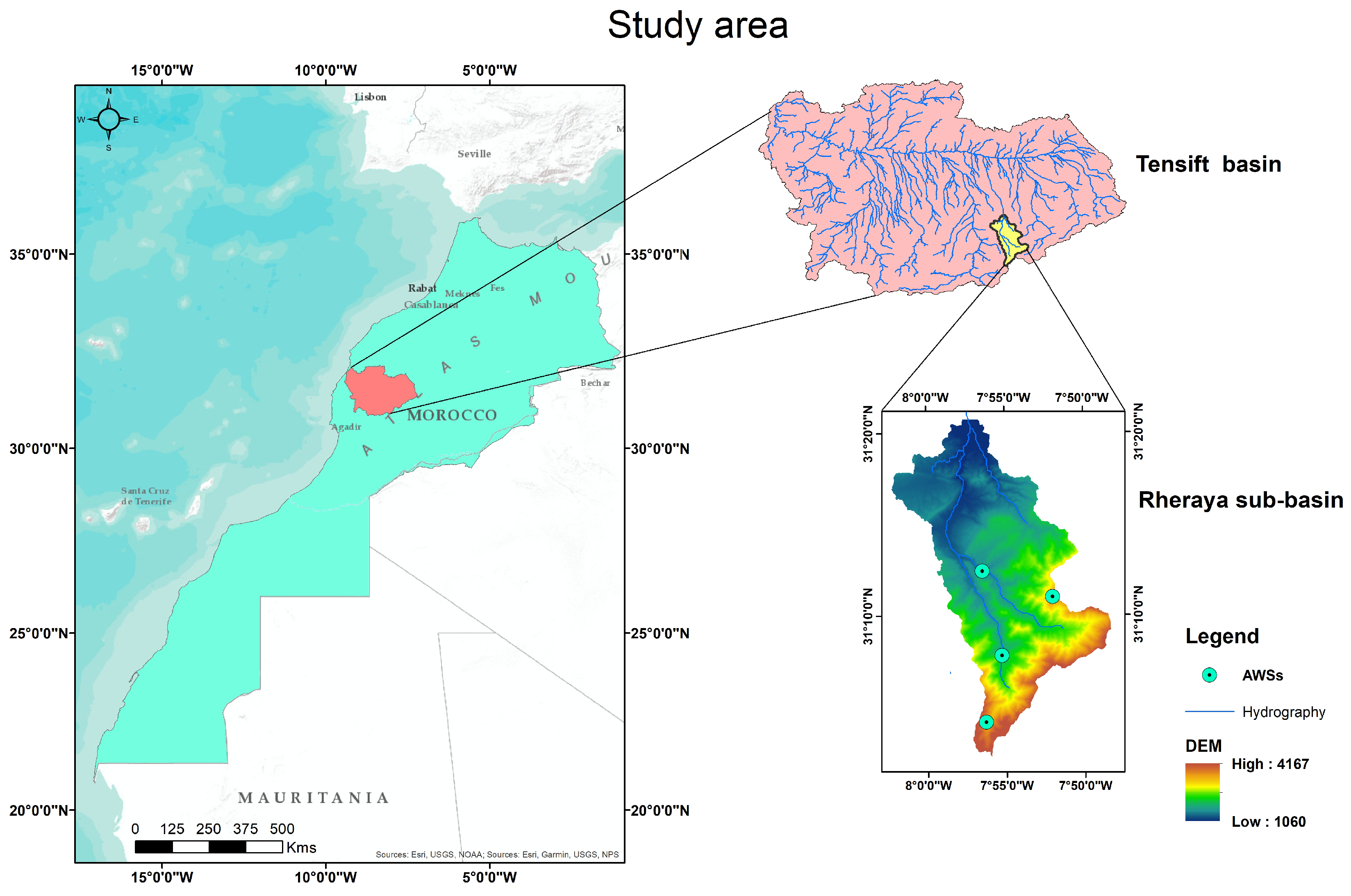
2.1. Study Area

The High Atlas is a large mountain range located in Morocco, stretching for 800 km in length and 60 km in width. It runs in a northeast to southwest direction and is known for its diverse range of elevations, from the lowest point of 1060 m above sea level to the highest peak in North Africa, Mount Toubkal, which reaches an elevation of 4167 m above sea level (Figure 1) [50,51]. The western part of the High Atlas is particularly notable for being a vital source of water for the northern plain of the Tensift catchment, specifically around the city of Marrakech [52].The high-altitude regions of the mountain range are known for their low temperatures and sparse vegetation cover, with most agricultural activities concentrated along river valleys [53,54]. The Rheraya sub-basin (Figure 1), which is located 40 km south of Marrakech (between latitudes 30°05 N and 30°20 N, and longitudes 7°40 W and 8°00 W) and covers an area of 225 km², is one of the most intensely studied areas of the High Atlas Mountains. It represents a part of the Tensift Observatory in the frame of the SudMed [52] and the Joint International Laboratory LMI-TREMA [55] (https://www.lmi-trema.ma/ last accessed on 26 January 2023) funded by the University Cadi Ayyad (UCA, Marrakech, Morocco) and the French Research Institute for Development (IRD, CESBIO Laboratory, Toulouse, France). It is considered to be globally representative of the western watershed of the High Atlas Mountains. The sub-basin contains four AWSs and is equipped with a variety of instruments to study the area.

2.2. Dataset

2.2.1. Observed Ground-Based Data

The air temperatures in the Rheraya sub-basin were measured on a semihourly basis from Automatc Weather Stations (AWSs) positioned throughout the sub-basin: Imskerbour (1404 m above sea level), Aremd (1940 m above sea level), Neltner (3207 m above sea level), and Oukaimden (3230 m above sea level). The temperature records for the period from 2016 to 2020 were converted from their original format to hourly timesteps, and any half-hour intervals with missing records from one or more AWSs were excluded. In order to ensure the accuracy of the data, the temperature records were checked for any excessive amounts of missing values, as outlined in the study of Dodson and Marks [56]. The missing values for the combined stations were ensured to not exceed 100 days per year. After the preprocessing step, the minimum number of hours kept per day for all years is 22 h/day. The locations of the stations are illustrated in Figure 1, and Table 1 provides detailed information on the station names, heights, coordinates, yearly mean temperatures, number of observations, and frequency.

2.2.2. Reanalysis Data

For this study, the most advanced global reanalysis data produced in Europe, specifically optimized for land surface applications, was used. The dataset used is the ERA5-Land enhanced global dataset for the land component of the fifth generation of European Reanalysis, which is freely available on the website https://cds.climate.copernicus.eu (last accessed on 26 January 2023) [57]. In comparison with ERA5 and the older ERA-Interim, the ERA5-Land dataset has the advantage of enhanced horizontal resolution of 9 km (released on a regular 0.1° × 0.1° grid) compared with 31 km (ERA5) and 80 km (ERA-Interim), while maintaining the same hourly temporal resolution as ERA5 [18]. The high temporal and spatial resolutions of ERA5-Land, and the consistency of the fields produced, make it a valuable dataset for diverse applications related to water resources, land, and environmental management. The variable of interest in this study is the air temperature at 2 m above the surface of land, sea or inland waters, which is calculated through interpolation between the lowest model level and the Earth’s surface, considering atmospheric conditions. Hourly ERA5-Land temperature data were downloaded and processed to be consistent with the measured data screening. Additionally, ERA5-Land temperature’s daily mean, minimum, maximum, and standard deviation were computed as ancillary data for the entire study period.

2.2.3. Digital Elevation Model
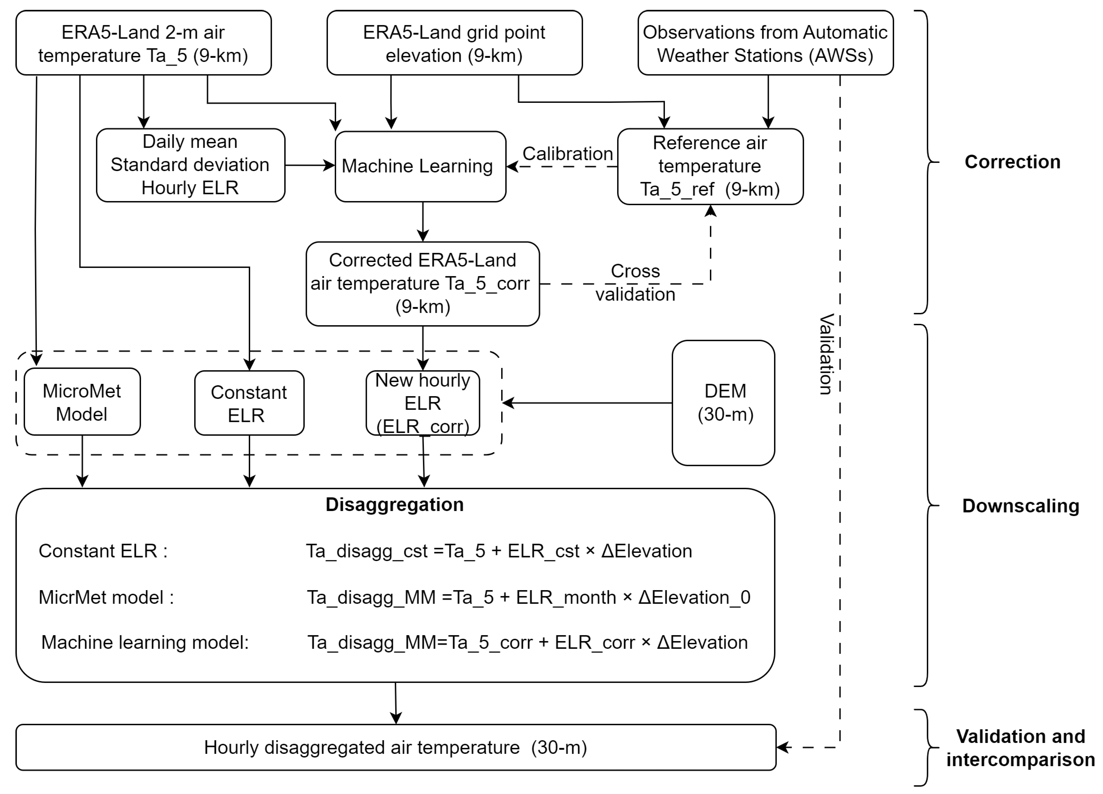
To achieve fine-scale disaggregation, we used the Shuttle Radar Topography Mission (SRTM) 1 Arc-Second Global digital elevation model (DEM) with 30 m resolution (https://earthexplorer.usgs.gov/ last accessed on 26 January 2023). The related SRTM 1 Arc-Second tile (SRTM1N31W008V3) was used to generate a DEM subset of the Rheraya sub-basin (Figure 1).

2.3. Methodology

In this section, we outline the process for enhancing the spatiotemporal downscaling of Ta. We first explain the use of machine learning models to correct ERA5-Land Ta (hereafter referred to as Ta_5) using in situ hourly Ta and ELR readings (Ta_st and ELR_st), resulting in corrected Ta_5 (Ta_5_corr). Then, we describe the process of using Ta_5_corr to downscale temperatures at a 30 meter resolution using a DEM, producing Ta_disagg_ML. This final product is validated against five years of in situ hourly Ta_st readings and compared with two other downscaling methods (Annual ELR average and MicroMet model) to evaluate the improvement made. Additional details on each step are provided in subsequent subsections.

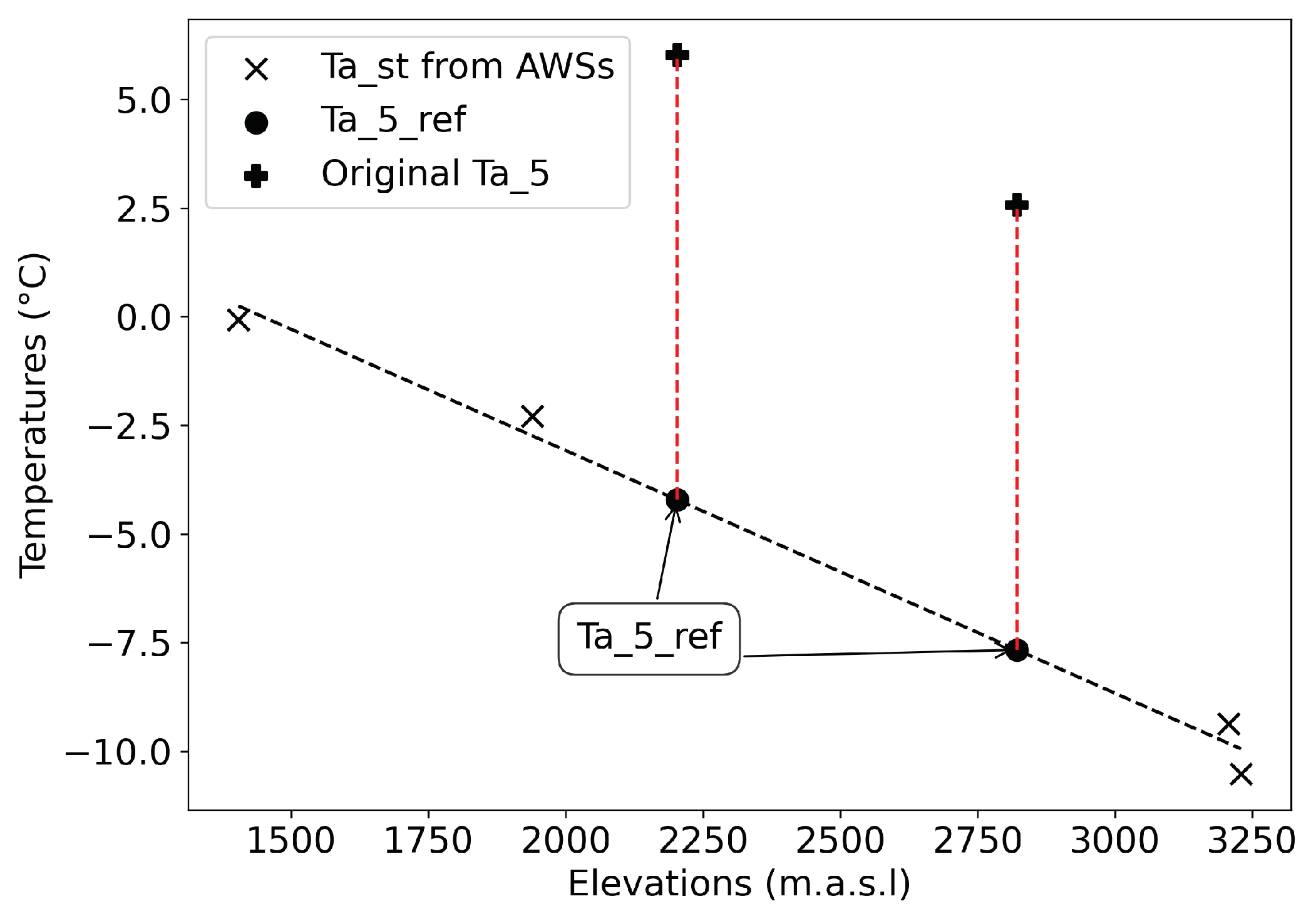
2.3.1. 1st Step: Ta_5 Correction

The process of correcting Ta_5 starts with the creation of a reference Ta (Ta_5_ref) corresponding to each 9 km ERA5-Land grid elevation, utilizing only ground data, specifically, hourly measured Ta_st and ELR_st. The Ta_5_ref is aligned with the measured Ta_st and ELR and is intended to be more accurate than the one provided by ERA5-Land, serving as the target to be achieved prior to downscaling. This step is illustrated in Figure 2. In the second step, using only ERA5-Land Ta_5, a set of variables is derived, which may be correlated with the local disaggregated temperature that is intended to be produced. This set of variables is then utilized in the machine learning approaches. In the third step, Ta_5 is corrected to match the Ta_5_ref (9-km spatial resolution) using machine learning models. In these models, the estimated value is Ta_5_corr, Ta_5_ref is the dependent variable, and the independent variables include Ta_5 and the selected variables from step 2.
The Ta_st measured by AWSs are plotted against their corresponding elevations, and linear regressions are used to calculate the slope hourly ELR_st and the intercept b_st (representing air temperature at sea-level). These values are then used to interpolate hourly Ta_5_ref for elevations of ERA5-Land grid points (9 km spatial resolution) over the period of interest (from 2016 to 2020). The equation that governs this interpolation is as follow (Equation (1):
Ta _ 5 _ ref = ELR _ st × E 5 + b _ st
E5 being the elevation of ERA5-Land grid point in meters.
These Ta_5_ref values are then used to calibrate machine learning models as a dependent variable to correct Ta_5. The input variables include Ta_5 and a set of variables potentially correlated with the local disaggregated temperature that is intended to be produced. The input features for predicting a specific variable may be highly correlated with one another, resulting in a processing and computational time loss. In addition, those input features may not always be correlated with the target variable, which can result in an overfitting of the constructed model. In other words, the learned model would be a better fit for training data than test data [58]. To avoid these problems, carrying out a correlation analysis holds the key to decide which inputs to keep or to exclude. The Pearson Correlation Coefficient (PCC) can be used to calculate the correlation between candidate input variables Xi and targeted variable Y. The PCC is by definition the covariance of X i and Y over the product of their standard deviations σ X i and σ Y . It ranges from −1 to +1, where a value of −1/+1 implies that X i is completely negatively/positively linearly correlated with Y, and a value of 0 indicates absolute absence of correlation between the two variables. In most cases, a high absolute value of PCC (often greater than 0.8) indicates strong correlation [58]. The expression of PCC is given in Equation (2):
PCC = C O V ( X i , Y ) σ X i × σ Y
The candidate variables selected for conducting the correlation analysis are hourly Ta_5, hourly ELR calculated using Ta_5 (hereafter referred as ELR_E5), daily Ta_5 means, minimums, maximums, standard deviations, and ERA5-Land grid points elevations. These variables are used to examine the correlation with the targeted variable, Ta_5_ref. The goal is to use the selected input variables, all of which are sourced from ERA5-Land data, to predict a more accurate corrected Ta_5_corr, which is applied for downscaling. We chose to test three different models for predicting Ta_5_ref: (1) a basic multiple-input linear regression method known as MLR, (2) the popular and widely used SVR model, and (3) one of the newest machine learning methods, the Xgboost algorithm, which is known for its exceptional predictive abilities. Next is a brief theoretical explanation of the operation and functioning of the models.
  • MLR
In MLR, multiple independent variables are used to describe the behavior of the dependent variable [59]. It is an extension of simple linear regression, and it describes the relationship between two or more explanatory variables and a response variable by fitting a linear equation to observed data. Each value of the independent variable corresponds to a prediction value for the dependent variable. A good MLR model should be able to explain a majority of the variance in the dependent variable with the smallest number of independent variables possible. For a more detailed explanation of MLR theory, the reader is encouraged to refer to the work of Helsel and Hirsch [60].
  • SVR
SVR is a branch of Support Vector Machine (SVM) that is widely used as a regression technique (detailed description of SVM can be found in several works, e.g., [61,62,63]). SVR finds a multivariate regression function that predicts a desired output property or dependent variable Y based on a set of input independent variables X (NxM) and Y (M). The main difference between SVR and MLR is that, in SVR, the original input space (which is usually nonlinearly related to the targeted variable) is mapped onto a higher-dimensional feature space using a kernel function (such as Linear, Radial Basis Function, Polynomial, and sigmoid) to find an optimal hyperplane to separate the sample points. The full description of SVR equations is not included here but can be found in works such as [64,65,66].
  • Xgboost
Xgboost, proposed by Chen et al. in 2015 [67], is an alternative method for predicting a response variable based on certain covariates. It is similar to the well-known Random Forest method: it builds classification and regression trees one by one, but instead of making a decision based on a final vote, each subsequent model (tree or base learner) is trained using the mistakes of the previous one. This technique is becoming increasingly popular due to its design and ability to speed up training time using various techniques such as parallel computing and sparsity-aware split-finding. For more details, the reader is referred to the following [34,67,68]
All the previously mentioned algorithms were implemented using the Python library “Scikit-learn” developed by Pedregosa et al. in 2011 [69]. Scaling was performed prior to using SVR kernel methods, as they are based on distance; this was performed to facilitate learning and prevent features with the largest range from dominating the computations. The “RobustScaler” method was used, as it can handle outliers. The performance of the machine learning models heavily depends on the hyperparameter values; therefore, a significant step was determining the optimal values for the model through hyperparameter tuning. This was conducted using the “Scikit-learn” library’s Grid Search function, which considers multiple hyperparameter combinations and chooses the one that returns the lowest error score. Since MLR model does not have any hyperparameters to tune, only SVR’s and Xgboost’s hyperparameters were tuned. The Grid search function also includes a predefined k-fold cross-validation method [70,71,72,73,74], where each fold serves as a single hold-out test fold, and the model is built using the remaining k-1 folds. Grid search methodology with 5-fold cross-validation was applied to obtain the optimal model parameters for SVR and Xgboost, meaning that during the cross-validation process, 4 years of data were used for calibration and 1 year of data for validation.

2.3.2. 2nd Step: Disaggregation

Climate impact studies frequently use a constant Ta lapse rate at specific locations, which we hereafter refer to as ELR_cst and which is equal to −6.5 C · km 1 (e.g., [75,76,77,78]). However, this rate can vary significantly depending on factors such as location, season, and time of day. Studies have shown that the temperature ELR can range from −9.8 C · km 1 to −10 C · km 1 in dry conditions (the dry adiabatic lapse rate), and values that are shallower or equal to −6.5 C · km 1 generally represent moist adiabatic conditions [28,79,80,81]. This variability was measured in our study area, as shown in Figure 3.
To account for this variability, the correction of ERA5-Land Ta_5 on an hourly basis enables tracking actual local ELR values. Once the models predict corrected temperature values Ta_5_corr, new hourly temperature lapse rates (ELR_corr) are computed through linear regression, and then the Ta_5_corr (9 km) is downscaled to the DEM of the area of interest (30 m) using those corrected values instead of the original ones. The equation used for this downscaling process is shown in Equation (4), and the classic constant Ta lapse rate method’s formula is displayed in Equation (3).
Ta _ disagg _ cst = Ta _ 5 + ELR _ cst × ( DEM E 5 )
Ta _ disagg _ ML = Ta _ 5 _ corr + ELR _ corr × ( DEM E 5 )
In addition to using machine learning and the constant Ta lapse rate approach to downscale Ta_5, the MicroMet model was also applied for comparison. The MicroMet model is a high-resolution meteorological distribution model designed to produce high-resolution meteorological data such as air temperature, humidity, wind, radiation, and precipitation for use in running spatially distributed terrestrial models over a variety of landscapes. It uses established relationships between meteorological variables and the surrounding landscape to distribute those variables in a computationally efficient and physically plausible way. Specifically for air temperature, the MicroMet model first adjusts the Ta_5 values to sea level using the formula (Equation (5)):
Ta _ 0 = Ta _ 5 + ELR _ month × ( E 5 E 0 )
Ta_0 and ELR_month being the Ta adjusted to sea level and the monthly values of the ELR, respectively (see Table 2), where the ELR_month values vary depending on the month of the year [82] or are calculated based on data from nearby stations. The sea-level Ta_0 values are then interpolated to the model grid using the Barnes objective analysis method [83]. The gridded topography data and ELR_month are then utilized to adjust the sea-level gridded temperatures to the elevations provided by the DEM, using the equation provided in Equation (6):
Ta _ disagg _ MM = Ta _ 0 + ELR _ month × ( DEM E 0 )

2.3.3. 3rd Step: Validation and Results Assessment

The quality of the final products (i.e., the downscaled Ta_disagg_ML) was evaluated through in situ validation and comparison with the other two scenarios (Ta_disagg_MM and Ta_disagg_cst) using statistical parameters. Three simulation evaluation scores were used: Root Mean Square (RMSE), coefficient of determination (R²), which is the square of the previously described PCC (Pearson’s Correlation Coefficient), and the Mean Bias Error (MBE) [84]. The scores were computed for each AWS for validation. The mathematical expressions of the above scores are presented in Equations (7) and (8) (R² is the square of PCC in Equation (2)).
MBE = 1 N i = 1 N ( P r e d i O b s i )
RMSE = 1 N i = 1 N ( P r e d i O b s i ) 2
P r e d i being the predicted value and O b s i the measured one. The above-mentioned steps and methodology description are summarized in the following flowchart (Figure 4). It provides a clear and concise summary of the method and can serve as a guide to understand and replicate the study’s methodology.

3. Results

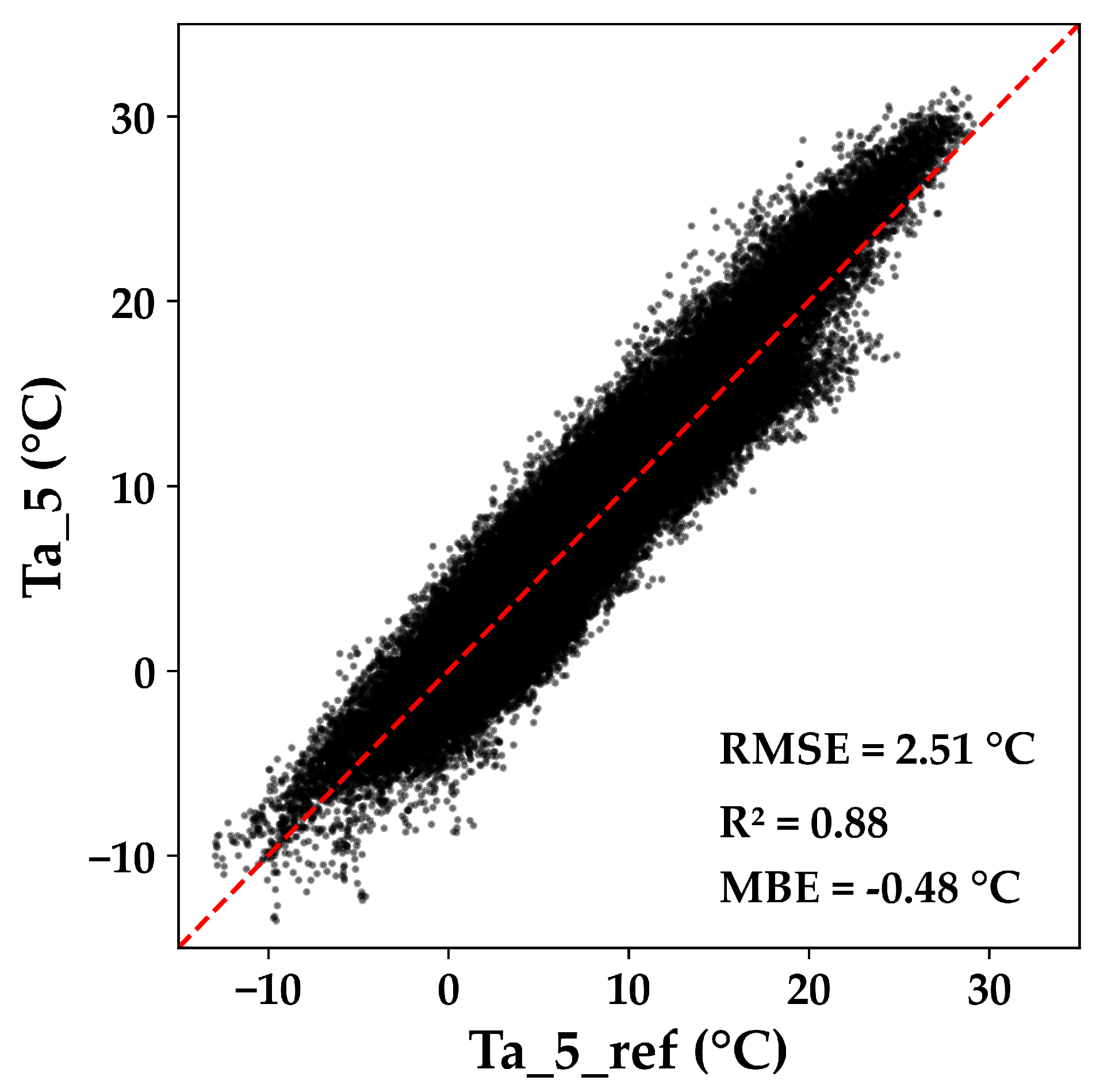
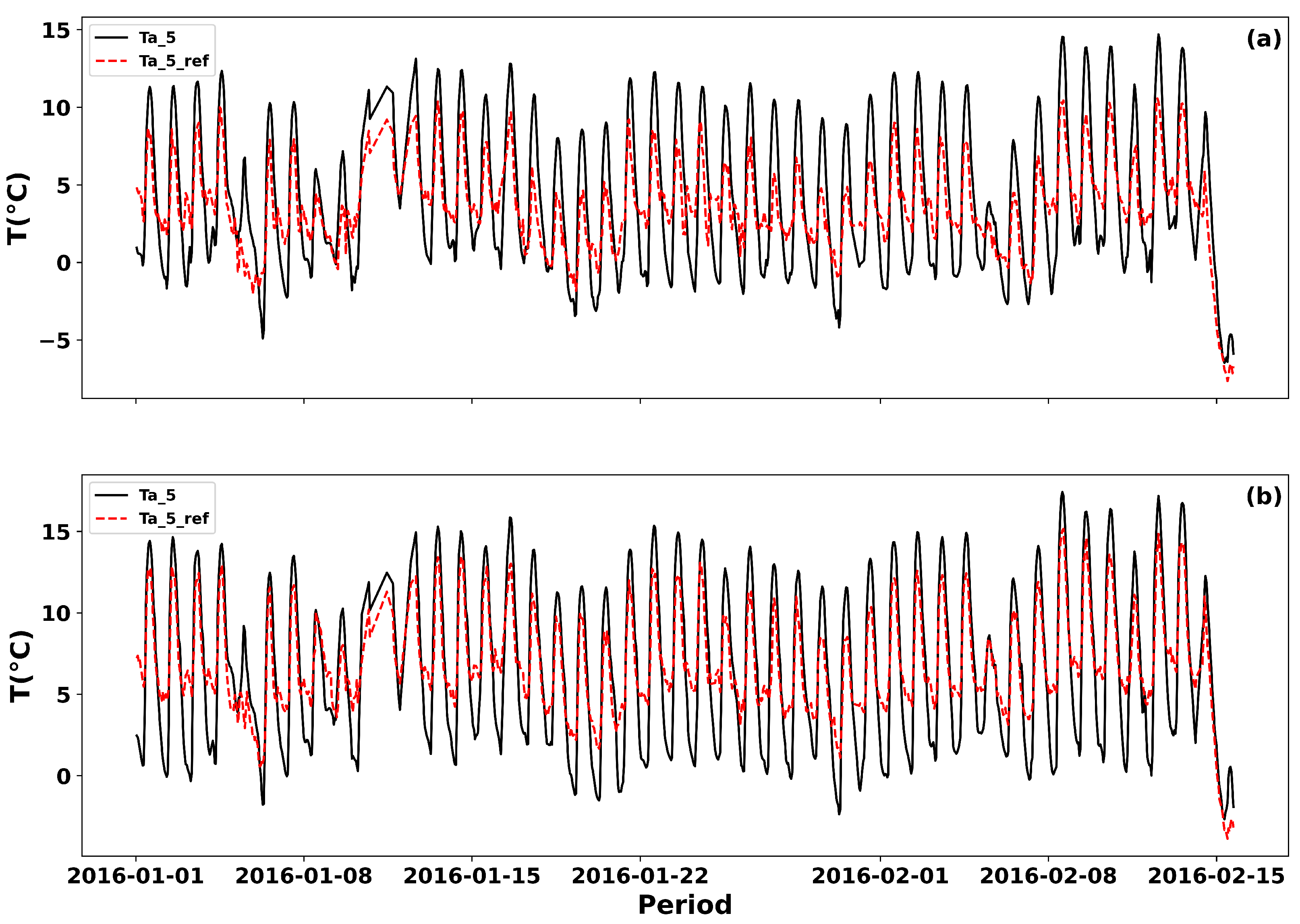
3.1. Ta_5 Correction

  • Reference temperature Ta_5_ref
The obtained hourly reference Ta_5_ref values were compared with the Ta_5 values sourced directly from ERA5-Land data. The comparison was carried out over all ERA5-Land grids and the entire study period (2016 to 2020). The results of this comparison are shown in Figure 5. The mean R², RMSE, and MBE of Ta_5_ref and Ta_5 were found to be 0.88, 2.51 C, and −0.48 C, respectively. The results indicate that the predicted values closely follow the reference values, however, the difference between the two can reach up to approximately 10 C.
The next figure (Figure 6) illustrate a temporal comparison of Ta_5_ref to the original Ta_5 for two ERA5-Land grids. The lines are plotted on top of each other, and the difference between the two temperatures can be easily observed. The figure shows an example of the comparison for two ERA5-Land grids over the first two and a half months of 2016, and similar behavior is observed throughout the study period.
The plot indicates that the trend of the two variables is similar, meaning that they both increase or decrease at the same rate over time. However, the amplitude of the Ta_5_ref variable is less than the amplitude of the original reanalysis Ta_5, meaning that the range of temperatures it covers is smaller. This suggests that the reanalysis Ta has higher amplitude of Ta variations than what it should be over the study area. The corrections to be applied to the Ta_5 are then to adjust for the bias that may present in the reanalysis dataset. This bias can be caused by errors in the input data, topographical effects, the modeling approach, or in the assimilation of observations. The bias can also be caused by the lack of representation of the complex topography or urbanization of the study area in the reanalysis dataset. At first, we attempted to debias/correct the Ta_5 using simple linear regression, modeling daily temperature changes as a sinusoidal function, and constant (positive or negative) bias correction prior to downscaling. However, these methods did not yield significant improvement and were not practical for the study area, hence the choice of the machine learning approaches. As we stated in the methodology section, a correlation analysis was carried out to select proper input variables prior to Ta_5 correction, and is thus based only on a set of variables independent from in situ data (Ta_5 and its derivates, as well as ERA5-Land grid points elevations).
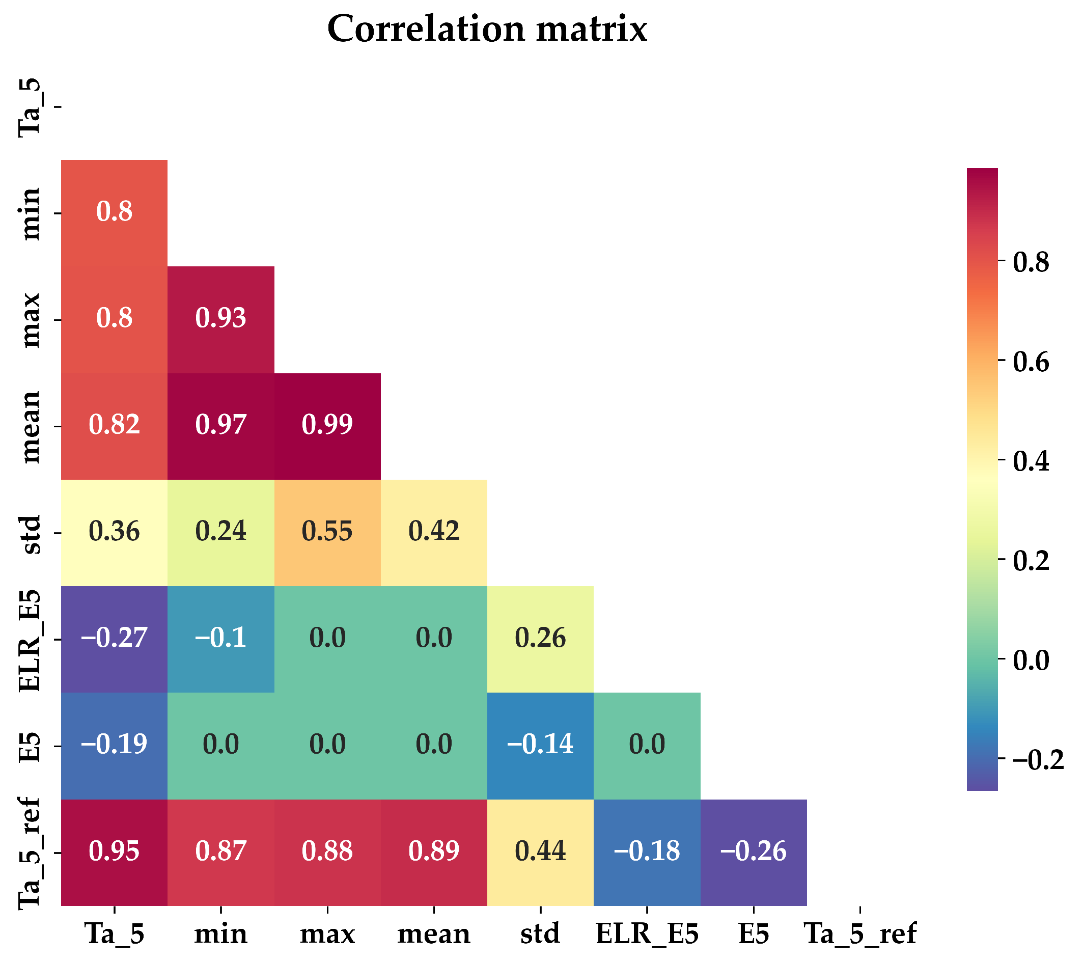
  • Correlation analysis and feature selection
Figure 7 depicts the results of the correlation analysis. To test for correlated input variables, the independent targeted variable Ta_5_ref was also introduced to the correlation matrix. The latter shows that Ta_5, Ta_5’s daily minimum, Ta_5’s daily maximum, and Ta_5’s daily mean are all highly correlated, with PCCs of 0.95, 0.87, 0.88, and 0.89, respectively. Moderately low to low correlations are found for standard deviation (PCC = 0.44), ELR_E5 (PCC = −0.18), and E5 (ERA5-Land’s grid elevation) (PCC = −0.26). Nonetheless, given our emphasis on finer resolution and higher precision, keeping those inputs appears to be very appropriate, as long as they are not very close to null (under 0.05 for instance).
The correlation matrix also shows that the daily mean of Ta_5 has almost perfect correlation with both the daily minimum and maximum values, with correlation coefficients of 0.97 and 0.99, respectively. Additionally, among the three, the daily mean showed the best correlation to the targeted variable Ta_5_ref (correlation coefficient of 0.89), thus only the mean was kept. The final set of retained input variables for predicting Ta_5_ref values (i.e., correcting Ta_5) consisted of five variables: Ta_5, Ta_5’s daily mean and standard deviation, and hourly ELR_E5 and E5 (ERA5-Land’s grid elevation). It is worth noting that while elevation remains constant over time, it varies from one ERA5-Land grid to the next, hence its inclusion was entirely justified.
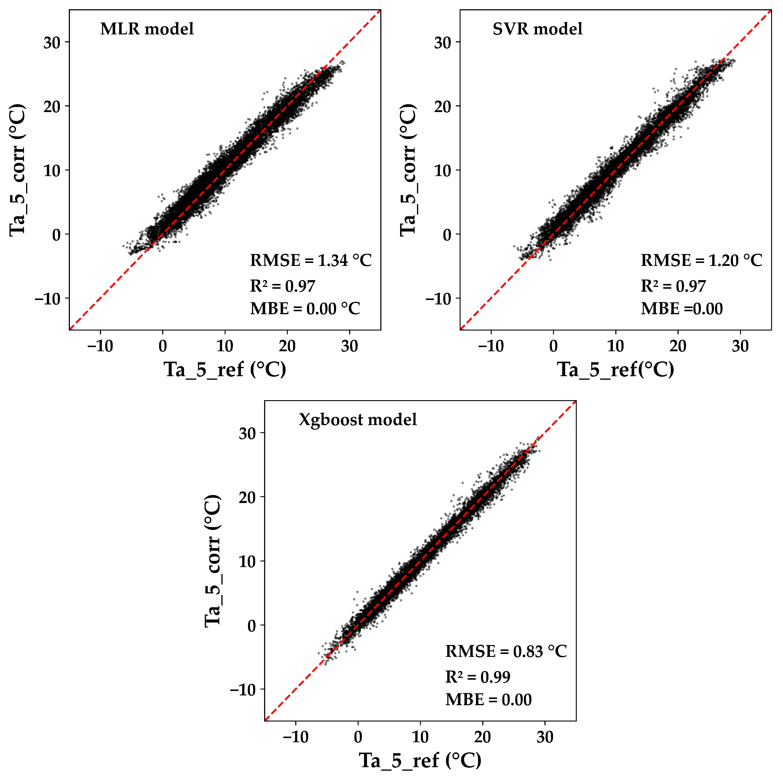
  • Machine learning outcome
The three scatterplots of Figure 8 compare the predictions of temperature made by the tested machine learning algorithms, MLR, SVR, and Xgboost, with the reference Ta_5_ref. Overall, the results show a good level of agreement between the predictions of the three models and the targeted reference Ta_5_ref.
The MLR-based model had an RMSE of 1.34 C, an R² of 0.97, and a quasi-null MBE. The fitting parameters of the MLR model are the coefficients of the regression equation used to predict the reference Ta_5_ref. They represent the contribution of each input feature in the linear equation. The specific values found for these fitting parameters are as follows: 0.507 for hourly Ta_5, 0.477 for daily mean, −3.17 × 10 3 for ERA5-Land grids elevation, −186.71 for hourly ELR_E5, −0.329 for daily standard deviation, and 6.27 for the intercept.
The SVR model used the Radial Basis Function (RBF) kernel, which is known to provide good general performance, as reported in previous studies such as Zaidi (2015) and Parveen et al. (2016). The grid search methodology along with 5-fold cross-validation was utilized to find the best values for the SVR model parameters, such as C, ϵ , and γ . A wide range of permutations were tried and tested, such as C [ 2 2 , 2 12 ], γ [ 2 12 , 2 2 ] and ϵ [ 2 12 , 2 4 ]. The statistical evaluation mean parameters for the best fitted SVR model were found to be RMSE = 1.20 C, R² = 0.97, and MBE=0 C using the Python package scikit-learn and the rules of “Lesser is better” for the RMSE and MBE and “Greater is better” for R². The best parameters found were C = 1, γ = “scale”, and ϵ = 0.02.
The grid search methodology was also applied to the Xgboost algorithm to find the best evaluation metrics (lowest RMSE and MBE and highest R2). An analysis of Aarshay’s (2016) work was used as a reference to determine typical values of learning rate, maximum depth, minimum child weight, gamma, subsample, and colsample by tree, such as [0.01,0.2], [3,10], [1,6], [0.1,0.2], [0.5,0.9], and [0.5,0.9]. The best fit was found when the following settings were used: learning rate = 0.4, maximum depth = 6, minimum child weight = 1, subsample = 1, colsample by tree = 1, and a “number of estimators” of 2000. The results from the Xgboost model are superior to those from the SVR model and MLR model, with an RMSE of 0.83 C, R² of 0.99, and MBE of 0 C, respectively. Table 3 displays the specific outcomes for the three scoring parameters from the various cross-validation folds. Overall, we see a consistent pattern of model behavior throughout each fold change process, indicating that the models are well-calibrated and are not overfitting.
To sum up, exceptional Ta_5 correction performance of the Xgboost model in predicting the reference Ta_5_ref was observed. The high R² value and low RMSE and MBE values indicate a better fit compared with the MLR and SVR models. Additionally, the Xgboost model stands out for its combination of both speed and accuracy, which is a significant advantage.

3.2. Ta_5_corr Downscaling

In this section, we present the results of our study on downscaling the 9 km ERA5-Land’s Ta_5 using three different scenarios. As a reminder, the three scenarios explored are our own method, the machine-learning-based method, and a comparison with classic downscaling approaches, the MicroMet model, as well as the often used constant ELR method (ELR_cst). As previously stated, the machine learning method was used to correct the Ta_5 values, and new values for ELR were calculated from the corrected Ta_5_corr values. These ELR_corr values are then used for the downscaling of the latter temperature. The results of each scenario are discussed in detail, and the comparison between them is highlighted.
Figure 9 highlights improvements made on ELR_corr estimations posterior to Ta_5 correction. The first subplot is a scatterplot of the ELR issued from noncorrected Ta_5 against the measured ELR_st from AWSs. The second subplot is a scatterplot of the machine-learning-based corrected ELR_corr against the measured ELR_st from AWSs (we are only showcasing the ELR_corr based on Ta_5_corr corrections made using Xgboost model, as it had the most favorable outcome).
The scatterplots show that there is a significant improvement in the agreement with the measured ELR_st when using the machine-learning-based approach ELR_corr. The R² value for the ELR_corr is 0.78, which is significantly higher than the R² value of 0.41 for the noncorrected ELR_E5. This indicates that the ELR_corr model has a better ability to accurately predict the measured ELR_st values from the AWSs. The constant ELR_cst and Micromet models’ monthly values (ELR_month) were not compared, as we would only obtain horizontal lines, given the fact that they are constant and the measured value ELR_st exhibits huge spatial temporal variability.
The results presented in Figure 10 show the performance of the three followed approaches for downscaling temperatures at 30 m resolution. The scatterplots compare the downscaled temperatures from each approach with the measured validation temperatures (Ta_st) from the four AWSs, Imeskerbour, Aremd, Neltner, and Oukaimden. The AWSs are displayed in columns, while the rows indicate the approach followed.
The first approach, using ELR_cst, the constant elevation-based lapse rate, and Ta_5, the original ERA5-Land’s temperature data, performed poorly, as expected, yielding an RMSE of 3.11 C, a coefficient of determination R² of 0.81, and an MBE of −0.55 C. Using the MicroMet model, the second approach did not improve the predictions either, although it outperformed the constant lapse rate model, with overall performance estimates of 2.71 C, 0.85, and −0.40 C for RMSE, R², and MBE, respectively.
The new machine-learning-based approach, which corrects Ta_5 temperature and lapse rate data prior to downscaling (Ta_5_corr and ELR_corr), showed a satisfying improvement in the match between the downscaled and measured temperatures. The intercomparison of the three machine learning models (Xgboost, SVR, and MLR) revealed that the Xgboost model had the best performance, with an RMSE of 1.61 C, an R² of 0.97, and an MBE of 0 C. The SVR model had a slightly worse performance with an RMSE of 1.75 C, an R² of 0.96, and an MBE of 0 C, but it took significantly more time to compute. The MLR model had the lowest performance, with RMSE = 1.8 C, R² = 0.96, and MBE = 0 C, but it still presents a satisfying improvement compared with constant elevation-based lapse rate and MicroMet models. The next table (Table 4) provides further details on the downscaling performance metrics by station and approach. The table shows that, overall, the constant lapse rate elevation-based approach and the MicroMet model present consistent RMSE for all the stations, however, the MBEs differ. These differences in relation to the measurements can be considered quite important, especially if the downscaled product is intended to be used as input for fine-scale models.
On the other hand, it is noted that all metrics are improved for all stations when using machine learning approaches. Additionally, it can be observed that the metrics for higher elevations (Oukaimden and Neltner) are better than those in lower elevations (Imskerbour and Aremd). This could be explained by several factors, such as the larger differences in temperature between the high and low elevations, or a better alignment to regression lines, and hence better corrected Ta_5_corr values. It could also be due to the fact that the machine learning models are able to capture the complex interactions between temperature and the ERA5-Land grid’s elevation in these regions more effectively.
In conclusion, the results of this study indicate that the present machine-learning-based downscaling technique has great potential for disaggregating ERA5-Land Ta_5 coarse 9 km resolution to the DEM’s 30 meter resolution, particularly in harsh and difficult-to-access mountainous regions. The use of machine learning models improved the performance of the downscaling process and the match between predicted and measured Ta. This approach outperforms the traditional constant elevation-based lapse rate and MicroMet model. Additionally, the Xgboost model was found to be the best option for reproducing this methodological approach, as it performed better and faster than the other two models (MLR and SVR).
The illustration presented in the next figure (Figure 11) depicts an example of mapping across the study region and summarizes the strategy followed to create a high-resolution downscaled air temperature based on 9 km ERA5-Land’s Ta_5 maps once the models are calibrated.

4. Discussion

The correction of ERA5-Land Ta_5 data through the application of machine learning techniques resulted in an enhanced spatial distribution of downscaled Ta estimates. The improvement was demonstrated through comparison with two classical downscaling methods: the annual average and the MicroMet model. To summarize, the process began with the creation of Ta_5_ref temperatures calculated for each ERA5-Land grid point’s elevation to match the observed local temperature–elevation relationship. In simpler terms, Ta_5_ref is a 9 km adjusted version of the ERA5-Land Ta_5 and a more accurate representation of the actual measurements of Ta_st and ELR_st. Hence, Ta_5_ref served as the desired outcome for the correction of Ta_5.
The gap between Ta_5 and Ta_5_ref values was filled through machine learning. Three different machine learning techniques, MLR (simple), SVR (relatively complex), and Xgboost (recent), were selected to make the prediction of Ta_5_ref. A correlation analysis was performed to determine the input variables that could be correlated with Ta_5_ref. These candidate input variables were all derived from the ERA5-Land data, meaning that once the models were calibrated, the Ta_5 temperature was corrected using its own data to align with the observed local temperature–elevation relationship before downscaling. The results of the correlation analysis show that the set of input variables is includes in addition to hourly Ta_5: hourly ELR_E5, the mean and standard deviation of daily Ta_5, and the elevation of the ERA5-Land grid points. The predicted/corrected values at 9 km spatial resolution, referred to as Ta_5_corr, were validated against Ta_5_ref and showed significant improvement. The original gap between Ta_5 and Ta_5_ref was quantified as having an RMSE of 2.51 C, an R² of 0.88, and an MBE of −0.48 C. The MLR-based model showed a correction with an RMSE of 1.34 C, an R² of 0.97, and a near-zero MBE. The best fit SVR model had an RMSE of 1.20 C, an R² of 0.97, and an MBE of 0 C. The Xgboost model performed even better, with an RMSE of 0.83 C, an R² of 0.99, and an MBE of 0 C, surpassing the results from the SVR and MLR models. The Ta_5_corr values at 9 km spatial resolution, more aligned with local measurements than the original Ta_5, were then used to calculate ELR_corr values. The resulting ELR_corr values were plotted against measurements and showed an R² of 0.78 and an RMSE of 0.001 C/km. The final product, the disaggregated Ta_5_disagg, was obtained by using Ta_5_corr and ELR_corr in conjunction with a 30 m DEM.
The downscaling results show a satisfying improvement in the match between downscaled Ta_5_disagg and measured Ta_st. The intercomparison of the three machine learning models (Xgboost, SVR, and MLR) revealed that the Xgboost model had the best performance, with an RMSE of 1.61 C, an R² of 0.97, and an MBE of 0 C. The SVR model had a slightly worse performance with an RMSE of 1.75 C, an R² of 0.96, and an MBE of 0 C, but it took significantly more time to compute. The MLR model had the lowest performance with RMSE = 1.8 C, R² = 0.96, and MBE = 0 C, but it still presents a satisfying improvement compared with the constant elevation-based lapse rate and MicroMet models. These differences in relation to the measurements can be considered quite important, especially if the downscaled product is intended to be used as input for fine-scale models.
The limitation of this method is that it needs a starting point, i.e., the machine learning models must be first calibrated accordingly to the reference temperature Ta_5_ref that is calculated through in situ measurements and ERA5-Land grid point elevations. The primary benefit, however, is that this is one of the few works that successfully downscales ERA5-Land Ta_5 to an hourly timestep, is applicable throughout all seasons, and captures both diurnal and regional temperature fluctuations. Moreover, once the models are calibrated over a specific area, they can be used independently of any knowledge of in situ measurements; as was previously mentioned, the inputs consist solely of ERA5-Land Ta_5 and its derived products (hourly ELR, daily mean, and standard deviation), in addition to ERA5-Land grid point elevations.

5. Conclusions

The ERA5-Land Ta_5 data were improved through the use of machine learning techniques in downscaling. The correction process started with the creation of Ta_5_ref, which is a 9 km adjusted version of the ERA5-Land Ta_5, better representing the actual temperature measurements. The gap between Ta_5 and Ta_5_ref was filled through machine learning using three models: MLR, SVR, and Xgboost. The results show that the Xgboost model performed the best, surpassing the SVR and MLR models. The downscaled product showed significant improvement compared with the one obtained through classic downscaling approachs (constant ELR and MicroMet model). The primary benefit of this method is that it can accurately downscale to an hourly timestep, is applicable throughout all seasons, and captures diurnal and regional temperature fluctuations. However, the models must be calibrated for a specific area before use. Overall, this method presents a promising solution for improving the accuracy of temperature data downscaling and can be used for other climate studies.
In perspective, assessment of the added value of this novel machine-learning-based method for hydrological applications is considered (e.g., reference evapotranspiration over mountains). Another avenue would be the extension of the use of machine learning models to downscale other meteorological variables (e.g., wind speed and relative humidity, etc.). Finally, although the time window would be more restrained, we can also consider the use of machine-learning-based methods on ERA5-Land’s Land Surface Temperature (LST) to reproduce high-resolution satellite products such as the thermal-based Landsat-8 LST.

Author Contributions

All the authors B.-e.S., S.K., O.M., V.S., C.E.H., M.H.K. and A.C. have contributed substantially to this manuscript. Conceptualization, B.-e.S.; methodology, B.-e.S.; software, B.-e.S. and C.E.H.; validation, B.-e.S.; formal analysis, B.-e.S., S.K., O.M., V.S., M.H.K. and A.C.; investigation, B.-e.S., S.K., O.M., V.S., M.H.K., and A.C.; resources, A.C.; data curation, B.-e.S., C.E.H.; writing—original draft preparation, B.-e.S.; writing—review and editing, B.-e.S., S.K., O.M., V.S., M.H.K., C.E.H. and A.C.; visualization, S.K., O.M., V.S. and A.C.; supervision, S.K., O.M., V.S. and A.C.; project administration, A.C.; funding acquisition, A.C. All authors have read and agreed to the published version of the manuscript.

Funding

This project has been financially supported by the OCP S.A. (Office Chérifien des Phosphates) in the context of ASSIWAT project (grant agreement no: 71), and The Horizon 2020 ACCWA project (grant agreement no: 823965) in the context of Marie Sklodowska-Curie research and the innovation staff exchange (RISE) program. The project PRIMA-S2-ALTOS-2018 “Managing water resources within Mediterranean agrosystems by Accounting for spatiaL sTructures and cOnnectivitieS are also acknowledged.

Institutional Review Board Statement

Not applicable.

Informed Consent Statement

Not applicable.

Data Availability Statement

Data sharing is not applicable to this article.

Acknowledgments

The authors acknowledge the data provided by theTensift Observatory as part of the SudMed program and the Joint International Laboratory LMI-TREMA (last accessed on 26 January 2023 at https://www.lmi-trema.ma/). Furthermore, they extend their appreciation to the academic editor and anonymous reviewers for their willingness to review the previous version of the manuscript.

Conflicts of Interest

The authors declare no conflict of interest.

Abbreviations and Symbols

The following abbreviations are used in this manuscript:
ELREnvironmental Lapse Rate
DEMDigital Elevation Model
AWSAutomatic Weather Station
MLRMultiple Linear Regression
SVRSupport Vector Regression
XgboostExtreme Gradient Boosting
TaAir temperature
Ta_5ERA5-Land’s air temperature
Ta_stMesaured air temperature
Ta_5_refReference air temperature based on ERA5-Land’s grid points elevation
Ta_5_corrMachine learning based corrected ERA5-Land’s air temperature
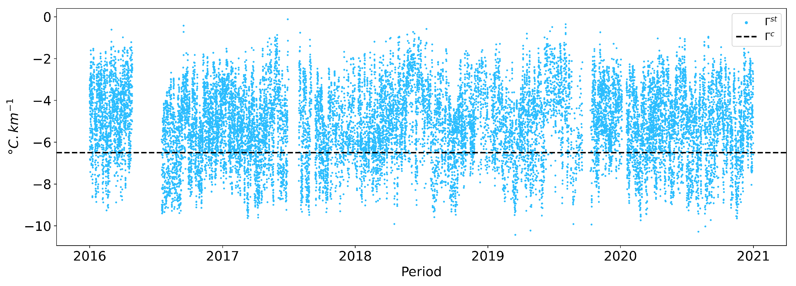
ELR_cstConstant ELR of a value of −6.5 C/km
ELR_E5Corresponding ERA5-Land ELR
ELR_stMeasured ELR
ELR_corrCorrected ELR based on ERA5-Land corrected air temperature
Ta_disagg_cstDownscaled ERA5-Land air temperaure based on constant ELR
Ta_disagg_MMDownscaled ERA5-Land air temperaure based on MicorMet model
Ta_disagg_MLDownscaled ERA5-Land air temperaure based on Machine learning models
MBEMean Bias Error
RMSERoot Mean Squared Error
PCCPearson Correlation Coefficient
E5ERA5-Land grid point elevation

References

  1. Maraun, D.; Wetterhall, F.; Ireson, A.; Chandler, R.; Kendon, E.; Widmann, M.; Brienen, S.; Rust, H.; Sauter, T.; Themeßl, M.; et al. Precipitation downscaling under climate change: Recent developments to bridge the gap between dynamical models and the end user. Rev. Geophys. 2010, 48. [Google Scholar] [CrossRef] [Green Version]
  2. Maselli, F.; Pasqui, M.; Chirici, G.; Chiesi, M.; Fibbi, L.; Salvati, R.; Corona, P. Modeling primary production using a 1 km daily meteorological data set. Clim. Res. 2012, 54, 271–285. [Google Scholar] [CrossRef] [Green Version]
  3. Tobin, C.; Rinaldo, A.; Schaefli, B. Snowfall limit forecasts and hydrological modeling. J. Hydrometeorol. 2012, 13, 1507–1519. [Google Scholar] [CrossRef]
  4. Behnke, R.; Vavrus, S.; Allstadt, A.; Albright, T.; Thogmartin, W.E.; Radeloff, V.C. Evaluation of downscaled, gridded climate data for the conterminous United States. Ecol. Appl. 2016, 26, 1338–1351. [Google Scholar] [CrossRef] [PubMed]
  5. Hewitt, C.D.; Stone, R.C.; Tait, A.B. Improving the use of climate information in decision-making. Nat. Clim. Chang. 2017, 7, 614–616. [Google Scholar] [CrossRef]
  6. Bjorkman, A.D.; Myers-Smith, I.H.; Elmendorf, S.C.; Normand, S.; Rüger, N.; Beck, P.S.; Blach-Overgaard, A.; Blok, D.; Cornelissen, J.H.C.; Forbes, B.C.; et al. Plant functional trait change across a warming tundra biome. Nature 2018, 562, 57–62. [Google Scholar] [CrossRef] [Green Version]
  7. Trisos, C.H.; Merow, C.; Pigot, A.L. The projected timing of abrupt ecological disruption from climate change. Nature 2020, 580, 496–501. [Google Scholar] [CrossRef]
  8. Fick, S.E.; Hijmans, R.J. WorldClim 2: New 1-km spatial resolution climate surfaces for global land areas. Int. J. Climatol. 2017, 37, 4302–4315. [Google Scholar] [CrossRef]
  9. Karger, D.N.; Conrad, O.; Böhner, J.; Kawohl, T.; Kreft, H.; Soria-Auza, R.W.; Zimmermann, N.E.; Linder, H.P.; Kessler, M. Climatologies at high resolution for the earth’s land surface areas. Sci. Data 2017, 4, 1–20. [Google Scholar] [CrossRef] [Green Version]
  10. Abatzoglou, J.T.; Dobrowski, S.Z.; Parks, S.A.; Hegewisch, K.C. TerraClimate, a high-resolution global dataset of monthly climate and climatic water balance from 1958 to 2015. Sci. Data 2018, 5, 1–12. [Google Scholar] [CrossRef] [Green Version]
  11. Navarro-Racines, C.; Tarapues, J.; Thornton, P.; Jarvis, A.; Ramirez-Villegas, J. High-resolution and bias-corrected CMIP5 projections for climate change impact assessments. Sci. Data 2020, 7, 1–14. [Google Scholar] [CrossRef] [PubMed] [Green Version]
  12. Hersbach, H.; Bell, B.; Berrisford, P.; Hirahara, S.; Horányi, A.; Muñoz-Sabater, J.; Nicolas, J.; Peubey, C.; Radu, R.; Schepers, D.; et al. The ERA5 global reanalysis. Q. J. R. Meteorol. Soc. 2020, 146, 1999–2049. [Google Scholar] [CrossRef]
  13. Gelaro, R.; McCarty, W.; Suárez, M.J.; Todling, R.; Molod, A.; Takacs, L.; Randles, C.A.; Darmenov, A.; Bosilovich, M.G.; Reichle, R.; et al. The modern-era retrospective analysis for research and applications, version 2 (MERRA-2). J. Clim. 2017, 30, 5419–5454. [Google Scholar] [CrossRef] [PubMed]
  14. Saha, S.; Moorthi, S.; Wu, X.; Wang, J.; Nadiga, S.; Tripp, P.; Behringer, D.; Hou, Y.T.; Chuang, H.y.; Iredell, M.; et al. The NCEP climate forecast system version 2. J. Clim. 2014, 27, 2185–2208. [Google Scholar] [CrossRef]
  15. Kalnay, E.; Kanamitsu, M.; Kistler, R.; Collins, W.; Deaven, D.; Gandin, L.; Iredell, M.; Saha, S.; White, G.; Woollen, J.; et al. The NCEP/NCAR 40-year reanalysis project. Bull. Am. Meteorol. Soc. 1996, 77, 437–472. [Google Scholar] [CrossRef]
  16. Kistler, R.; Kalnay, E.; Collins, W.; Saha, S.; White, G.; Woollen, J.; Chelliah, M.; Ebisuzaki, W.; Kanamitsu, M.; Kousky, V.; et al. The NCEP–NCAR 50-year reanalysis: Monthly means CD-ROM and documentation. Bull. Am. Meteorol. Soc. 2001, 82, 247–268. [Google Scholar] [CrossRef]
  17. Kobayashi, S.; Ota, Y.; Harada, Y.; Ebita, A.; Moriya, M.; Onoda, H.; Onogi, K.; Kamahori, H.; Kobayashi, C.; Endo, H.; et al. The JRA-55 reanalysis: General specifications and basic characteristics. J. Meteorol. Soc. Jpn. Ser. II 2015, 93, 5–48. [Google Scholar] [CrossRef] [Green Version]
  18. Muñoz-Sabater, J.; Dutra, E.; Agustí-Panareda, A.; Albergel, C.; Arduini, G.; Balsamo, G.; Boussetta, S.; Choulga, M.; Harrigan, S.; Hersbach, H.; et al. ERA5-Land: A state-of-the-art global reanalysis dataset for land applications. Earth Syst. Sci. Data 2021, 13, 4349–4383. [Google Scholar] [CrossRef]
  19. Holden, Z.A.; Abatzoglou, J.T.; Luce, C.H.; Baggett, L.S. Empirical downscaling of daily minimum air temperature at very fine resolutions in complex terrain. Agric. For. Meteorol. 2011, 151, 1066–1073. [Google Scholar] [CrossRef]
  20. Zhang, H.; Pu, Z.; Zhang, X. Examination of errors in near-surface temperature and wind from WRF numerical simulations in regions of complex terrain. Weather. Forecast. 2013, 28, 893–914. [Google Scholar] [CrossRef] [Green Version]
  21. Le Roux, R.; Katurji, M.; Zawar-Reza, P.; Quénol, H.; Sturman, A. Comparison of statistical and dynamical downscaling results from the WRF model. Environ. Model. Softw. 2018, 100, 67–73. [Google Scholar] [CrossRef]
  22. Alessi, M.J.; DeGaetano, A.T. A comparison of statistical and dynamical downscaling methods for short-term weather forecasts in the US N ortheast. Meteorol. Appl. 2021, 28, e1976. [Google Scholar] [CrossRef]
  23. Zhang, G.; Zhu, S.; Zhang, N.; Zhang, G.; Xu, Y. Downscaling hourly air temperature of WRF simulations over complex topography: A case study of Chongli District in Hebei Province, China. J. Geophys. Res. Atmos. 2022, 127, e2021JD035542. [Google Scholar] [CrossRef]
  24. Vrac, M.; Drobinski, P.; Merlo, A.; Herrmann, M.; Lavaysse, C.; Li, L.; Somot, S. Dynamical and statistical downscaling of the French Mediterranean climate: Uncertainty assessment. Nat. Hazards Earth Syst. Sci. 2012, 12, 2769–2784. [Google Scholar] [CrossRef] [Green Version]
  25. Vigaud, N.; Vrac, M.; Caballero, Y. Probabilistic downscaling of GCM scenarios over southern India. Int. J. Climatol. 2013, 33, 1248–1263. [Google Scholar] [CrossRef]
  26. Dulière, V.; Zhang, Y.; Salathé, E.P., Jr. Extreme precipitation and temperature over the US Pacific Northwest: A comparison between observations, reanalysis data, and regional models. J. Clim. 2011, 24, 1950–1964. [Google Scholar] [CrossRef] [Green Version]
  27. Wang, J.; Fonseca, R.M.; Rutledge, K.; Martín-Torres, J.; Yu, J. A hybrid statistical-dynamical downscaling of air temperature over Scandinavia using the WRF model. Adv. Atmos. Sci. 2020, 37, 57–74. [Google Scholar] [CrossRef]
  28. Dutra, E.; Muñoz-Sabater, J.; Boussetta, S.; Komori, T.; Hirahara, S.; Balsamo, G. Environmental lapse rate for high-resolution land surface downscaling: An application to ERA5. Earth Space Sci. 2020, 7, e2019EA000984. [Google Scholar] [CrossRef] [Green Version]
  29. Ekström, M.; Grose, M.R.; Whetton, P.H. An appraisal of downscaling methods used in climate change research. Wiley Interdiscip. Rev. Clim. Chang. 2015, 6, 301–319. [Google Scholar] [CrossRef]
  30. Soares, P.M.; Cardoso, R.M.; Miranda, P.; de Medeiros, J.; Belo-Pereira, M.; Espirito-Santo, F. WRF high resolution dynamical downscaling of ERA-Interim for Portugal. Clim. Dyn. 2012, 39, 2497–2522. [Google Scholar] [CrossRef]
  31. Aitken, M.L.; Kosović, B.; Mirocha, J.D.; Lundquist, J.K. Large eddy simulation of wind turbine wake dynamics in the stable boundary layer using the Weather Research and Forecasting Model. J. Renew. Sustain. Energy 2014, 6, 033137. [Google Scholar] [CrossRef] [Green Version]
  32. Laprise, R.; De Elia, R.; Caya, D.; Biner, S.; Lucas-Picher, P.; Diaconescu, E.; Leduc, M.; Alexandru, A.; Separovic, L. Challenging some tenets of regional climate modelling. Meteorol. Atmos. Phys. 2008, 100, 3–22. [Google Scholar] [CrossRef]
  33. Warrach-Sagi, K.; Schwitalla, T.; Wulfmeyer, V.; Bauer, H.S. Evaluation of a climate simulation in Europe based on the WRF–NOAH model system: Precipitation in Germany. Clim. Dyn. 2013, 41, 755–774. [Google Scholar] [CrossRef] [Green Version]
  34. Pan, B. Application of XGBoost algorithm in hourly PM2.5 concentration prediction. In Proceedings of the IOP Conference Series: Earth and Environmental Science; IOP Publishing: Bristol, UK, 2018; Volume 113, p. 012127. [Google Scholar]
  35. Cao, B.; Gruber, S.; Zhang, T. REDCAPP (v1. 0): Parameterizing valley inversions in air temperature data downscaled from reanalyses. Geosci. Model Dev. 2017, 10, 2905–2923. [Google Scholar] [CrossRef] [Green Version]
  36. Winstral, A.; Jonas, T.; Helbig, N. Statistical downscaling of gridded wind speed data using local topography. J. Hydrometeorol. 2017, 18, 335–348. [Google Scholar] [CrossRef]
  37. Stahl, K.; Moore, R.; Floyer, J.; Asplin, M.; McKendry, I. Comparison of approaches for spatial interpolation of daily air temperature in a large region with complex topography and highly variable station density. Agric. For. Meteorol. 2006, 139, 224–236. [Google Scholar] [CrossRef]
  38. Overland, J.E.; Wang, M. Recent extreme Arctic temperatures are due to a split polar vortex. J. Clim. 2016, 29, 5609–5616. [Google Scholar] [CrossRef]
  39. Jylhä, K.; Tuomenvirta, H.; Ruosteenoja, K. Climate change projections for Finland during the 21 st century. Boreal Environ. Res. 2004, 9, 127–152. [Google Scholar]
  40. Hanssen-Bauer, I.; Achberger, C.; Benestad, R.; Chen, D.; Førland, E. Statistical downscaling of climate scenarios over Scandinavia. Clim. Res. 2005, 29, 255–268. [Google Scholar] [CrossRef] [Green Version]
  41. Hofstra, N.; Haylock, M.; New, M.; Jones, P.; Frei, C. Comparison of six methods for the interpolation of daily, European climate data. J. Geophys. Res. Atmos. 2008, 113. [Google Scholar] [CrossRef] [Green Version]
  42. Tripathi, S.; Srinivas, V.; Nanjundiah, R.S. Downscaling of precipitation for climate change scenarios: A support vector machine approach. J. Hydrol. 2006, 330, 621–640. [Google Scholar] [CrossRef]
  43. Pardo-Igúzquiza, E.; Chica-Olmo, M.; Atkinson, P.M. Downscaling cokriging for image sharpening. Remote Sens. Environ. 2006, 102, 86–98. [Google Scholar] [CrossRef] [Green Version]
  44. Rodriguez-Galiano, V.; Pardo-Igúzquiza, E.; Sanchez-Castillo, M.; Chica-Olmo, M.; Chica-Rivas, M. Downscaling Landsat 7 ETM+ thermal imagery using land surface temperature and NDVI images. Int. J. Appl. Earth Obs. Geoinf. 2012, 18, 515–527. [Google Scholar] [CrossRef]
  45. Ho, H.C.; Knudby, A.; Sirovyak, P.; Xu, Y.; Hodul, M.; Henderson, S.B. Mapping maximum urban air temperature on hot summer days. Remote Sens. Environ. 2014, 154, 38–45. [Google Scholar] [CrossRef]
  46. Waichler, S.R.; Wigmosta, M.S. Development of hourly meteorological values from daily data and significance to hydrological modeling at HJ Andrews Experimental Forest. J. Hydrometeorol. 2003, 4, 251–263. [Google Scholar] [CrossRef]
  47. Sourp, L.; Gascoin, S.; Wassim Baba, M.; Deschamps-Berger, C. Development of a snow reanalysis pipeline using downscaled ERA5 data: Application to Mediterranean mountains. In Proceedings of the EGU General Assembly Conference Abstracts, Vienna, Austria, 23–27 May 2022; p. EGU22–5117. [Google Scholar]
  48. Liston, G.E.; Elder, K. A meteorological distribution system for high-resolution terrestrial modeling (MicroMet). J. Hydrometeorol. 2006, 7, 217–234. [Google Scholar] [CrossRef] [Green Version]
  49. Liston, G.E.; Elder, K. A distributed snow-evolution modeling system (SnowModel). J. Hydrometeorol. 2006, 7, 1259–1276. [Google Scholar] [CrossRef] [Green Version]
  50. Chaponnière, A.; Boulet, G.; Chehbouni, A.; Aresmouk, M. Understanding hydrological processes with scarce data in a mountain environment. Hydrol. Process. Int. J. 2008, 22, 1908–1921. [Google Scholar] [CrossRef] [Green Version]
  51. Boudhar, A.; Duchemin, B.; Hanich, H.; Chaponnière, A.; Maisongrande, P.; Boulet, G.; Stitou, J.; Chehbouni, A. Analysis of snow cover dynamics in the Moroccan High Atlas using SPOT-VEGETATION data. Sci. Chang. Planét./Sécher. 2007, 18, 278–288. [Google Scholar]
  52. Chehbouni, A.; Escadafal, R.; Duchemin, B.; Boulet, G.; Simonneaux, V.; Dedieu, G.; Mougenot, B.; Khabba, S.; Kharrou, H.; Maisongrande, P.; et al. An integrated modelling and remote sensing approach for hydrological study in arid and semi-arid regions: The SUDMED Programme. Int. J. Remote Sens. 2008, 29, 5161–5181. [Google Scholar] [CrossRef] [Green Version]
  53. Driouech, F.; Déqué, M.; Mokssit, A. Numerical simulation of the probability distribution function of precipitation over Morocco. Clim. Dyn. 2009, 32, 1055–1063. [Google Scholar] [CrossRef]
  54. Bouras, E.H.; Jarlan, L.; Er-Raki, S.; Balaghi, R.; Amazirh, A.; Richard, B.; Khabba, S. Cereal yield forecasting with satellite drought-based indices, weather data and regional climate indices using machine learning in Morocco. Remote Sens. 2021, 13, 3101. [Google Scholar] [CrossRef]
  55. Jarlan, L.; Khabba, S.; Er-Raki, S.; Le Page, M.; Hanich, L.; Fakir, Y.; Merlin, O.; Mangiarotti, S.; Gascoin, S.; Ezzahar, J.; et al. Remote sensing of water resources in semi-arid Mediterranean areas: The joint international laboratory TREMA. Int. J. Remote Sens. 2015, 36, 4879–4917. [Google Scholar] [CrossRef]
  56. Dodson, R.; Marks, D. Daily air temperature interpolated at high spatial resolution over a large mountainous region. Clim. Res. 1997, 8, 1–20. [Google Scholar] [CrossRef]
  57. Muñoz-Sabater, J.; Lawrence, H.; Albergel, C.; Rosnay, P.; Isaksen, L.; Mecklenburg, S.; Kerr, Y.; Drusch, M. Assimilation of SMOS brightness temperatures in the ECMWF Integrated Forecasting System. Q. J. R. Meteorol. Soc. 2019, 145, 2524–2548. [Google Scholar] [CrossRef]
  58. Liu, Y.; Mu, Y.; Chen, K.; Li, Y.; Guo, J. Daily activity feature selection in smart homes based on pearson correlation coefficient. Neural Process. Lett. 2020, 51, 1771–1787. [Google Scholar] [CrossRef]
  59. Sachindra, D.; Huang, F.; Barton, A.; Perera, B. Least square support vector and multi-linear regression for statistically downscaling general circulation model outputs to catchment streamflows. Int. J. Climatol. 2013, 33, 1087–1106. [Google Scholar] [CrossRef] [Green Version]
  60. Helsel, D.R.; Hirsch, R.M. Statistical Methods in Water Resources; Elsevier: Amsterdam, The Netherlands, 1992; Volume 49. [Google Scholar]
  61. Boser, B.E.; Guyon, I.M.; Vapnik, V.N. A training algorithm for optimal margin classifiers. In Proceedings of the Fifth Annual Workshop on Computational Learning Theory, Pittsburgh, PA, USA, 27–29 July 1992; pp. 144–152. [Google Scholar]
  62. Cortes, C.; Vapnik, V. Support-vector networks. Mach. Learn. 1995, 20, 273–297. [Google Scholar] [CrossRef]
  63. Gunn, S.R. Support vector machines for classification and regression. ISIS Tech. Rep. 1998, 14, 5–16. [Google Scholar]
  64. Vapnik, V. The Nature of Statistical Learning Theory; Springer Science & Business Media: Berlin, Germany, 1999. [Google Scholar]
  65. Cristianini, N.; Shawe-Taylor, J. An Introduction to Support Vector Machines and Other Kernel-Based Learning Methods; Cambridge University Press: Cambridge, UK, 2000. [Google Scholar]
  66. Schölkopf, B.; Smola, A.J.; Bach, F. Learning with Kernels: Support Vector Machines, Regularization, Optimization, and Beyond; MIT Press: Cambridge, MA, USA, 2002. [Google Scholar]
  67. Chen, T.; He, T.; Benesty, M.; Khotilovich, V.; Tang, Y.; Cho, H.; Chen, K. Xgboost: Extreme Gradient Boosting, R Package Version 0.4-2; 2015, Volume 1, pp. 1–4. Available online: https://cran.r-project.org/web/packages/xgboost/vignettes/xgboost.pdf (accessed on 1 March 2023).
  68. Pesantez-Narvaez, J.; Guillen, M.; Alcañiz, M. Predicting motor insurance claims using telematics data—XGBoost versus logistic regression. Risks 2019, 7, 70. [Google Scholar] [CrossRef] [Green Version]
  69. Pedregosa, F.; Varoquaux, G.; Gramfort, A.; Michel, V.; Thirion, B.; Grisel, O.; Blondel, M.; Prettenhofer, P.; Weiss, R.; Dubourg, V.; et al. Scikit-learn: Machine learning in Python. J. Mach. Learn. Res. 2011, 12, 2825–2830. [Google Scholar]
  70. Stone, M. Cross-validation: A review. Stat. J. Theor. Appl. Stat. 1978, 9, 127–139. [Google Scholar]
  71. Mohr, M.; Tveito, O. Daily temperature and precipitation maps with 1 km resolution derived from Norwegian weather observations. In Proceedings of the 13th Conference on Mountain Meteorology/17th Conference on Applied Climatology, Citeseer, Whistler, BC, Canada, 11–15 August 2008; pp. 11–15. [Google Scholar]
  72. Sluiter, R. Interpolation Methods for the Climate Atlas; KNMI: De Bilt, The Netherlands, 2012. [Google Scholar]
  73. Hengl, T.; Heuvelink, G.; Perčec Tadić, M.; Pebesma, E.J. Spatio-temporal prediction of daily temperatures using time-series of MODIS LST images. Theor. Appl. Climatol. 2012, 107, 265–277. [Google Scholar] [CrossRef] [Green Version]
  74. Aalto, J.; Pirinen, P.; Heikkinen, J.; Venäläinen, A. Spatial interpolation of monthly climate data for Finland: Comparing the performance of kriging and generalized additive models. Theor. Appl. Climatol. 2013, 112, 99–111. [Google Scholar] [CrossRef]
  75. Minder, J.R.; Mote, P.W.; Lundquist, J.D. Surface temperature lapse rates over complex terrain: Lessons from the Cascade Mountains. J. Geophys. Res. Atmos. 2010, 115. [Google Scholar] [CrossRef] [Green Version]
  76. Shen, Y.J.; Shen, Y.; Goetz, J.; Brenning, A. Spatial-temporal variation of near-surface temperature lapse rates over the Tianshan Mountains, central Asia. J. Geophys. Res. Atmos. 2016, 121, 14,006–14,017. [Google Scholar] [CrossRef]
  77. Wang, Y.; Wang, L.; Li, X.; Chen, D. Temporal and spatial changes in estimated near-surface air temperature lapse rates on Tibetan Plateau. Int. J. Climatol. 2018, 38, 2907–2921. [Google Scholar] [CrossRef] [Green Version]
  78. Jobst, A.M.; Kingston, D.G.; Cullen, N.J.; Sirguey, P. Combining thin-plate spline interpolation with a lapse rate model to produce daily air temperature estimates in a data-sparse alpine catchment. Int. J. Climatol. 2017, 37, 214–229. [Google Scholar] [CrossRef]
  79. Pepin, N.C. The Possible Effects of Climate Change on the Spatial and Temporal Variation of the Altitudinal Temperature Gradient and the Consequences for Growth Potential in the Uplands of Northern England. Ph.D. Thesis, Durham University, Durham, UK, 1994. [Google Scholar]
  80. Shuttleworth, W.J. Terrestrial Hydrometeorology; John Wiley & Sons: New York, NY, USA, 2012. [Google Scholar]
  81. Li, Y.; Zeng, Z.; Zhao, L.; Piao, S. Spatial patterns of climatological temperature lapse rate in mainland China: A multi–time scale investigation. J. Geophys. Res. Atmos. 2015, 120, 2661–2675. [Google Scholar] [CrossRef]
  82. Kunkel, K.E. Simple procedures for extrapolation of humidity variables in the mountainous western United States. J. Clim. 1989, 2, 656–669. [Google Scholar] [CrossRef]
  83. Koch, S.E.; DesJardins, M.; Kocin, P.J. An interactive Barnes objective map analysis scheme for use with satellite and conventional data. J. Appl. Meteorol. Climatol. 1983, 22, 1487–1503. [Google Scholar] [CrossRef]
  84. Kato, T. Prediction of photovoltaic power generation output and network operation. In Integration of Distributed Energy Resources in Power Systems; Elsevier: Amsterdam, The Netherlands, 2016; pp. 77–108. [Google Scholar]
Figure 1. Location of the Tensift basin and Rheraya sub-basin.
Atmosphere 14 00610 g001
Figure 2. Example of Ta_5_ref estimates for ERA5-Land grid elevations based on observed hourly ELR_st (slope). The dashed black line represents the regression line of measured temperature to elevation. The red dashed lines show the difference of ERA5-Land Ta_5 to Ta_5_ref (what it should be).
Atmosphere 14 00610 g002
Figure 3. Pronounced ELR’s hourly temporal variability, measured using AWS records over the period of interest (from 1 January 2016 to 31 December 2020).
Atmosphere 14 00610 g003
Figure 4. Flowchart of the methodological approach.
Atmosphere 14 00610 g004
Figure 5. Comparison of ERA5-Land’s original Ta_5 and reference Ta_5_ref air temperatures.
Atmosphere 14 00610 g005
Figure 6. Hourly Comparison of Ta_5 and reference Ta_5_ref over time (as dashed red line and black line, respectively). Example of the ERA5-Land grid situated at (a) 7.9° W and 31.1° N, and (b) 7.9° W and 31.2° N.
Atmosphere 14 00610 g006
Figure 7. Correlation matrix results. PCC value of each two variables is shown in the boxes corresponding to their “coordinates”. ELR_E5, Std and E5 being the hourly ELR issued from Ta_5, the daily standard deviation, and ERA5-Land grids elevation, respectively.
Atmosphere 14 00610 g007
Figure 8. Comparison of Machine Learning predictions for Ta_5_ref temperature.
Atmosphere 14 00610 g008
Figure 9. Comparison of noncorrected and corrected Ta_5 resulting ELRs.
Atmosphere 14 00610 g009
Figure 10. Performance evaluation of machine-learning-based ERA5-Land’s temperature downscaling against traditional Methods using In Situ measurements.
Atmosphere 14 00610 g010
Figure 11. High-resolution temperature mapping of mountainous regions using machine-learning-based downscaling of ERA5-Land’s T2m data. Example showing Xgboost in action across the Rheraya basin on 10 October 2021, at 11 a.m., after the initial calibration of the model.
Atmosphere 14 00610 g011
Table 1. Information regarding the four AWSs installed in the Rheraya sub-basin. The data collection period for all stations extends from 1 January 2016 to 31 December 2020.
AWSLatitudeLongitudeElevation (m.a.s.l)Tmean ( C)No. of ObservationsFrequency
Imskerbour31.21018°−7.93972°140415.0640,87030 min
Aremd31.12948°−7.91967°194012.143,84830 min
Neltner31.06579°−7.91389°32076.0443,82930 min
Oukaimden31.19328°−7.86546°32305.8542,64430 min
Table 2. Air temperature ELR ( C · km 1 ) variations for each month of the year in the Northern Hemisphere [82].
MonthJanuaryFebruaryMarchAprilMayJuneJulyAugustSeptemberOctoberNovemberDecember
ELR4.45.97.17.88.18.28.18.17.76.85.54.7
Table 3. Detailed cross-validation results.
Cross-Validation (Years)MLRSVRXgboost
RMSE R 2 MBERMSE R 2 MBERMSE R 2 MBE
20161.38780.95000.37401.22130.96900.26220.84110.98770.0240
20171.35420.9584−0.19441.24560.9654−0.21870.82320.9874−0.0123
20181.29350.9670−0.01291.18280.9733−0.01120.78910.9870−0.0116
20191.33100.96540.10791.21740.96960.11090.82600.9872−0.0031
20201.32340.9660−0.27341.17890.9750−0.16080.81390.9871−0.0104
Mean1.340.970.0021.210.97−0.0040.830.99−0.003
Table 4. Downscaling performance metrics by station and approach.
AWSRMSE R 2 MBE
Cst ELRMicroMetML ModelsCst ELRMicroMetML ModelsCst ELRMicroMetML Models
MLRSVRXgboost MLRSVRXgboost MLRSVRXgboost
Imskerbour2.452.711.821.861.750.900.880.950.940.95−0.430.280.340.420.34
Aremd3.092.472.051.951.770.840.90.930.940.95−2.14−0.70−0.50−0.45−0.49
Neltner3.293.001.611.551.410.760.810.940.950.95−0.49−0.670.100.020.08
Oukaimden3.472.671.681.621.470.750.820.940.940.950.86−0.540.100.000.08
Disclaimer/Publisher’s Note: The statements, opinions and data contained in all publications are solely those of the individual author(s) and contributor(s) and not of MDPI and/or the editor(s). MDPI and/or the editor(s) disclaim responsibility for any injury to people or property resulting from any ideas, methods, instructions or products referred to in the content.

