Article

Distribution and Meteorological Control of PM2.5 and Its Effect on Visibility in Northern Thailand

by
Teerachai Amnuaylojaroen
1,2,*,
Phonwilai Kaewkanchanawong
1 and
Phatcharamon Panpeng
1
1
Department of Environmental Science, School of Energy and Environment, University of Phayao, Phayao 56000 1, Thailand
2
Atmospheric Pollution and Climate Research Unit, School of Energy and Environment, University of Phayao, Phayao 56000 2, Thailand
*
Author to whom correspondence should be addressed.
Atmosphere 2023, 14(3), 538; https://doi.org/10.3390/atmos14030538
Submission received: 21 February 2023 / Revised: 7 March 2023 / Accepted: 10 March 2023 / Published: 11 March 2023
(This article belongs to the Special Issue Haze and Related Aerosol Air Pollution in Remote and Urban Areas)

Abstract

:
In the dry season, the north of Thailand always experiences reduced air quality, reduced visibility, and public health exposure from the burning of biomass domestically and in surrounding countries. The purpose of this research was to investigate the distribution and the meteorological control of PM2.5 accumulation, as well as its effect on visibility in northern Thailand in 2020. The Geographic Information System (GIS) was applied for the analysis of the spatial distribution, while Pearson’s correlation coefficient was utilized to examine the association between PM2.5 and meteorological variables. The results showed that the PM2.5 concentrations were in the range of 16–195 μg/m3 in 2020. The high level of PM2.5 in Lampang, Chiang Rai, and Chiang Mai provinces was in the range of 150 to 195 μg/m3 from January to May. Favorable meteorological conditions included low wind and relative humidity, and high temperatures contributed to high PM2.5 concentrations in northern Thailand. Domestic burning and burning in neighboring countries contribute to huge amounts of smoke that cause low visibility in northern Thailand, especially at 1 km above ground level, with a reduced visibility in the range of 70–90% for all provinces in April.

1. Introduction

In Southeast Asia, agricultural wastes are eliminated by crop management through the use of fires as well as deforestation for cropland [1,2]. This normally happens during the dry season, around November to April, as a result of extensive fire emissions at the onset of the Asian summer monsoon [3,4]. Simultaneously, a layer of temperature inversion from high pressure is present in many Southeast Asian countries, such as Thailand, Laos, and Burma, which, in conjunction with the increasing fire activity, contributes to the air quality problem in this region [3]. Previous studies have demonstrated that fire emission is the primary factor influencing ambient air quality in Mainland Southeast Asia, particularly for particulate matter with an aerodynamic width of less than 2.5 m (PM2.5) [3,5].
Air pollution from biomass burning is a common occurrence in northern Thailand, which is located in the north of the peninsula of Southeast Asia. This is particularly apparent from January to April [3]. Concerns regarding the region’s air quality are made worse by the large amount of biomass emissions coming from domestic sources and nearby countries including Burma, Laos, Vietnam, and Cambodia [6,7]. Furthermore, the problem of air pollution in northern Thailand is probably dominated by a mix of meteorological and geographic factors. Weather conditions that exacerbate particle matter building, burning of stubble in advance of impending rain and crop planting, and the multiple areas in northern Thailand’s narrow hills that serve as desirable basins for air pollutants all contribute to air pollution [8,9].
In order to properly assess and manage PM2.5 pollution, it is crucial to quantify the main contributing factors. According to previous research [10,11], weather factors can considerably disperse, remove, and induce pollutants as well as exert an influence on long-term variations in PM2.5. As a result, the distribution of PM2.5 is largely determined by weather patterns [12]. To support the government and policymakers in managing air quality, several previous studies have suggested a forecasting model for PM2.5 based on the association between meteorological factors and particulate matter. For example, Akbal and Ünlü [13] revealed the use of an advanced deep learning approach to expand understanding of particulate matter prediction by applying advanced machine learning with several trained methodologies, including Gaussian process regression, random forest regression (FRF), two different types of support vector machines (SVM), and artificial neural networks (ANN), which used meteorological factors as explanatory variables to predict PM2.5 [14]. Based on ANN along with k-mean clustering, principal component analysis (PCA) that contains wind speed and direction, temperature, precipitation, relative humidity, and solar radiation is also performed to forecast PM2.5 [15]. A hybrid deep learning method that includes the coupling of wavelet transformation and ANN with different structures and several meteorological data points including temperature, wind direction, and humidity also had good performance in forecasting PM2.5 [16]. As such, Akdi et al. [17] recently developed harmonic regression (HR), which is a univariate time series modeling approach that has advantages over classical time series approaches.
Low atmospheric visibility, which is a direct result of high-level particulate accumulation, provides the public with the clearest understanding of air quality, and it has been typically utilized as a surrogate for pollutant concentrations during times and in places where there were no monitoring systems for air quality [18]. For instance, severe air pollution was recently characterized by haze weather, which is described as an atmospheric occurrence with horizontal visibility less than 10 km caused by the dispersion of huge fine particles [19]. Both the general public and the scientific community were very concerned about this phenomenon [20,21,22]. Studies conducted in the past have investigated the relationship between meteorological variables and ambient air pollution. For instance, Yang et al. [21] determined that weather-related factors were responsible for 1.8 of the 15 µg/m3/decade variation in PM2.5 in the east of China between 1985 and 2005. According to a study by Zhang et al. [23], between 2013 and 2017 the proportionate contribution of climatic factors to large polluting events in the Beijing–Tianjin–Hebei region was stronger than 50%. Many studies have also attempted to establish a connection between PM2.5 and atmospheric visibility [24,25]. Due to geographical variations in air pollution and meteorological conditions as well as various analytic techniques, these earlier investigations, which were primarily conducted in a single city, have showed conflicting results. Therefore, in order to fill these information gaps, a study on the impact of PM2.5 on visibility was performed in multiple cities in northern Thailand throughout a haze episode. Furthermore, relationships between meteorological factors, such as relative humidity, surface temperature, wind speed, and PM2.5, were studied to improve the understanding of those patterns during the haze period in northern Thailand.

2. Materials and Methods

To analyze PM2.5 pollution and its effect on visibility in northern Thailand, several datasets, including ground-based measurements from the Pollution Control Department (PCD) in northern Thailand, the aerosol optical depth (AOD) data from Modern-Era Retrospective Analysis for Research and Applications version 2 (MERRA-2), and satellite images from both the Visible Infrared Imaging Radiometer Suite (VIIRS) of the National Oceanic and Atmospheric Administration (NOAA)-20 and the VIIRS-National Polar Partnership (NPP) were used for the analysis. The Pearson correlation was applied to analyze the relationship between PM2.5 and meteorological factors using data from the ground-based measurement of PCD in northern Thailand. Spatial analysis of PM2.5 and AOD was performed by Geographical Information System (GIS)-based Inverse Distance Weighted (IDW) interpolation.

2.1. Study Area and Air Pollution Data

We acquired hourly averaged pollution data from the Thai Pollution Control Department (PCD) in northern Thailand. Individual data were provided, including PM2.5, temperature, wind speed, and relative humidity at 3 m. We only considered background monitors with just enough data (about 25% missing data [26]) to verify that they represented the full period. As a result, the quantity of monitors with sufficient data was reduced to seven, as indicated in Table 1. Figure 1 illustrates the seven urban ground-monitoring stations chosen for this study. The quality assurance and quality control (QA/QC) systems relied on protocols established by the United States Environmental Protection Agency (EPA) [27]. The sampling performance criterion required the collection of quantifiable data on all PM2.5 exposures and microenvironmental concentrations. QA was guided by the following principles: (1) all processes must be thoroughly designed, tested, and implemented in accordance with standard operating procedures approved by the research director; (2) all data must be easily traceable; and (3) any deviations and irregularities must be documented [27].

2.2. Data Used

We used the aerosol optical depth (AOD) data from Modern-Era Retrospective analysis for Research and Applications version 2 (MERRA-2, M2IMNXGAS), which provide monthly mean data for this study. The data include an assimilation of both aerosol optical depth analysis increment and aerosol optical depth analysis. The data also contain the parameter variation. In addition, this dataset is the most recent version of global atmospheric reanalysis for the satellite that spans from 1980 to the present with a lag of approximately three weeks following the end of each month (https://disc.gsfc.nasa.gov/datasets/M2IMNXGAS_5.12.4/summary, accessed on 9 March 2023).
The Visible Infrared Imaging Radiometer Suite (VIIRS)—National Polar-orbiting Partnership (NPP) satellite image was utilized to determine the trajectory of the smoke plume in northern Thailand. This confluence of wavelengths is referred to as real color or natural color. The images depict land surface, sea, and atmospheric characteristics that appear natural. Only near real-time imagery of the Visible Infrared Imaging Radiometer Suite (VIIRS) Corrected Reflectance is available. The VIIRS sensor is on the Suomi National Polar-orbiting Partnership (NPP) satellite, which is a joint mission between NASA and NOAA. Worldview and the Global Imagery Browse Services can visualize the imagery (GIBS) with a resolution of 750 m and 375 m for M Bands and I Bands, respectively.
In this investigation, the satellite image of fire from VIIRS NOAA-20 was utilized. The Fire layer of the VIIRS displays active fire detection systems and heating anomalies. The layer of fire is important for investigating the distribution in terms of spatiality and temporality of fire, locating recurring hot spots, and identifying the air pollution source from a plume that may have negative health effects on humans. Sensor resolution is 375 m, picture resolution is 250 m, and temporal resolution is twice each day. The temperature anomalies are shown as red dots (approximate center of a 375 m pixel). The nominal observation times (equator crossover) for VIIRS S-NPP are 1:30 p.m. and 1:30 a.m., while NOAA-20 operates approximately 50 min ahead of S-NPP. Due to its polar orbit, mid-latitudes will receive three to four looks per day.

2.3. Data Analysis

To analyze the relationship between PM2.5 and meteorological variables including wind speed, surface temperature, and relative humidity, the Pearson correlation coefficient in Equation (1) was utilized in this study.
r = n ( x y ) ( x ) ( y ) [ n x 2 ( x ) 2 ] [ n y 2 ( y ) 2 ]
where r is correlation coefficient, while x and y represent values of the x and y variable in a sample.
The Pearson correlation coefficient (r) is a linear correlation coefficient that can be used to assess two or more correlated items. Due to the fact that it can indicate the degree of linear association between atmospheric parameters and air pollutants, it can serve as a measure of linearity. It can take values ranging from −1 to 1. A perfect linear relationship (r = −1 or r = 1) means that one of the variables can be perfectly explained by a linear function of the other.
Meanwhile, spatial analysis was described using interpolated maps that were transformed to raster images (about 30 m resolution) and categorized to depict the distribution of the number of participants in the research area using inverse distance weighted classification (IDW). The IDW interpolation determines cell values by linearly weighting a series of sample points. The inverse distance determines the weight. The extrapolated surface might be that of a variable that is position-dependent. This method assumes that the effect of the factor being mapping reduces as one moves away from the sampled location. The parameters of the interpolated surface can also be changed by limiting the amount of input points used in the calculation of each output cell value. By restricting the amount of input points analyzed, processing times can be reduced. Consider that input points located far from the cell location where the prediction is being made may have little or no spatial connection and so may be removed from the calculation [28,29].
The IDW approach, which is based on the concept of distance weighting, is utilized to interpolate spatial data in this study. This method is useful for estimating unknown depth data based on known (near) recorded depths. Equations (2) and (3) provide the IDW formulas:
R = i = 1 N w i R i
w i = d i α i = 1 N d i α
where R represents the unknown depth data (cm), Ri represents the depth data measured (cm), N is the number of points (in the search radius area), di is the distance from each depth to the calculated grid node, α is the power and is also a control parameter, generally assumed to be two, and wire presents the weighting of each depth.
The visibility was estimated as follows (4), which is based on work by Baumer et al. [30]:
V a = 3.912   ( Z i ) A O D 500 1
This approach also assumes that all aerosol is located within the mixing layer with a height of Zi. Where V a is the maximum horizontal distance that the human eye can see, Z i is constant with values of 1.0, 1.5, and 3 km [31], and A O D 500 is the AOD at 500 nm.

3. Results and Discussion

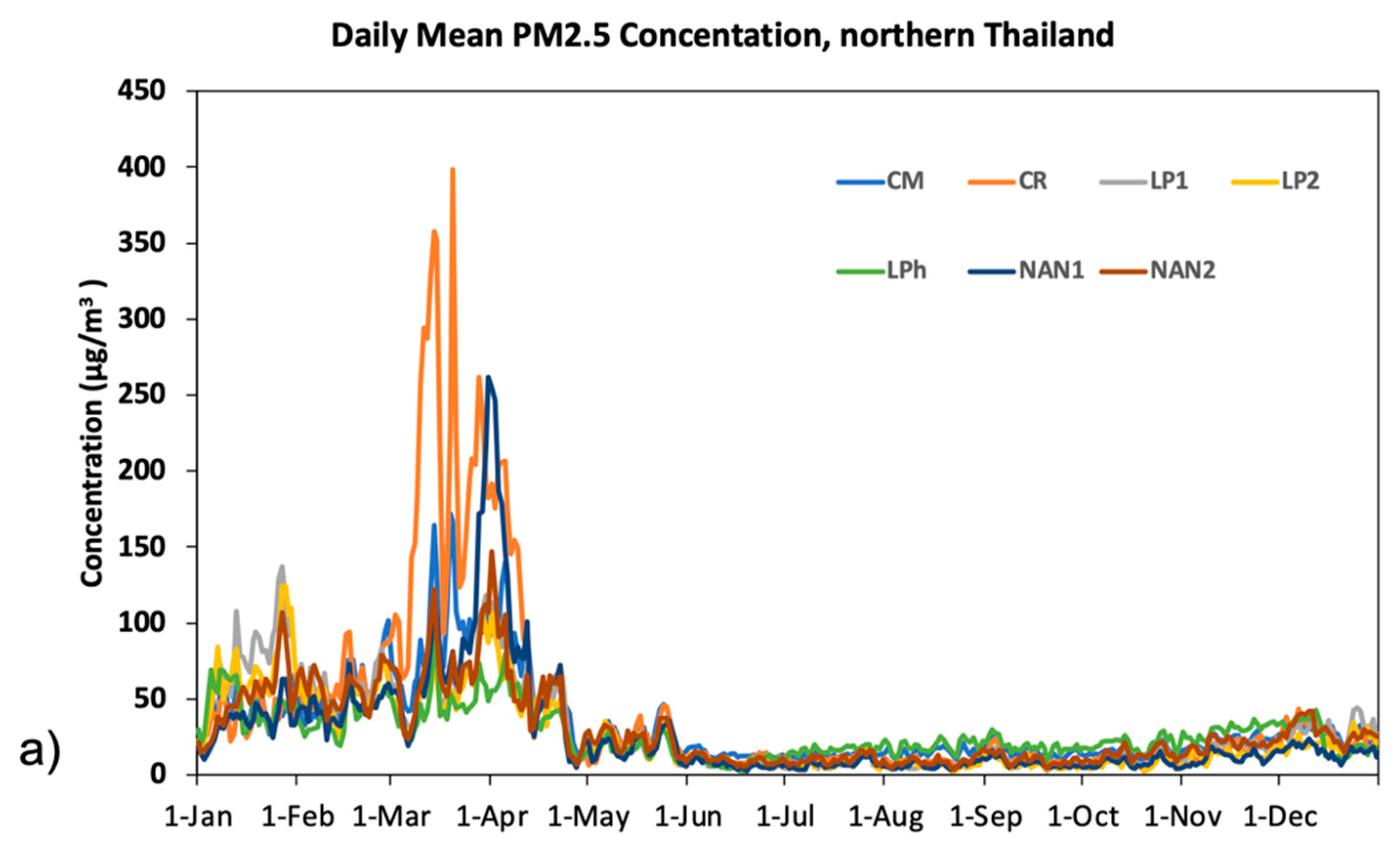
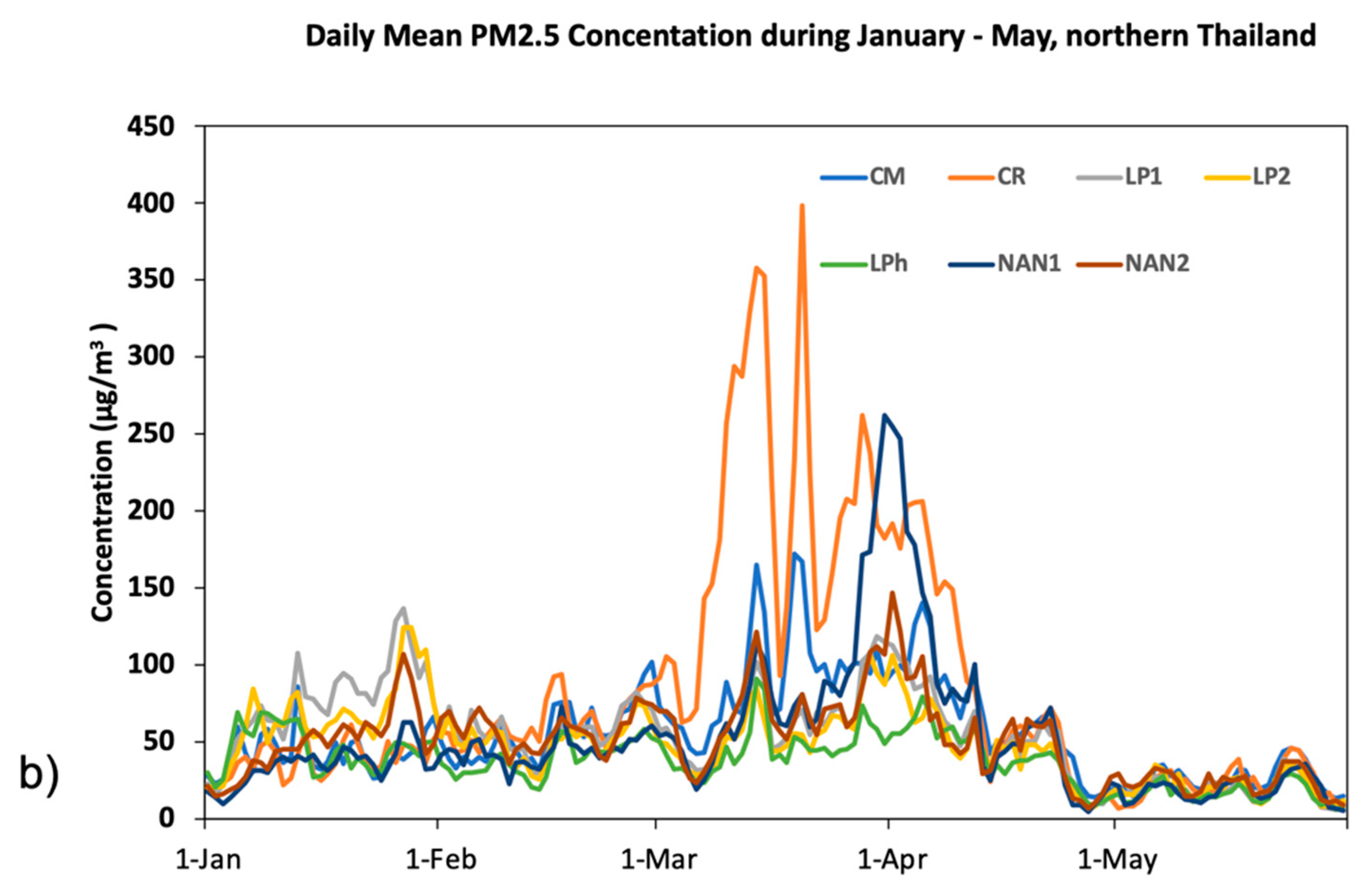
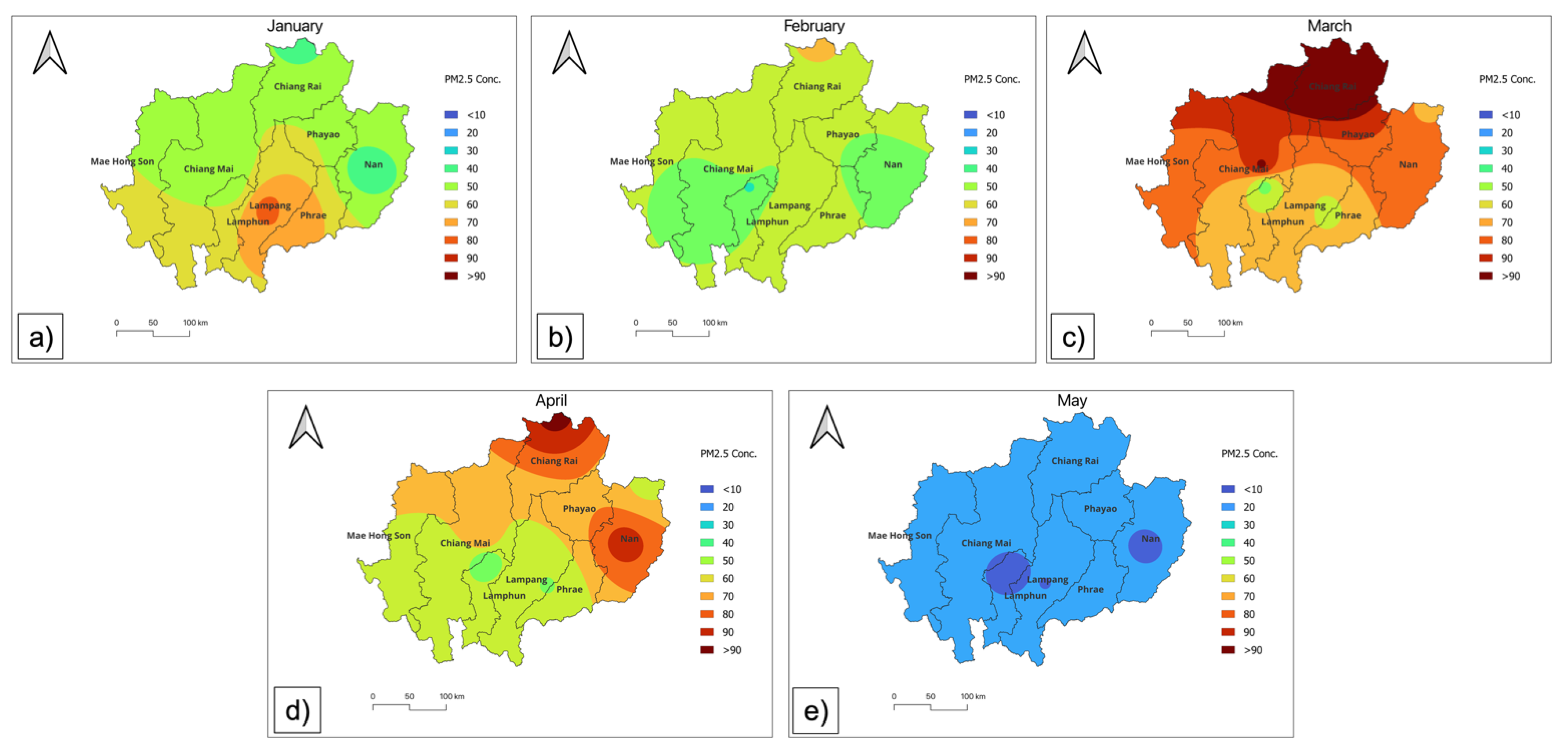
3.1. PM2.5 Monitoring in Northern Thailand

Figure 2 illustrates the daily PM2.5 concentrations in five provinces, including Chiang Mai, Chiang Rai, Lampang, Lamphun, and Nan in northern Thailand in 2020. The daily average of PM2.5 concentrations was higher than both Thailand’s and the USEPA’s guidelines, particularly from January to May. The highest levels of PM2.5 concentrations were found largely from March to April. The seasonal changes in emissions in this region are very certainly influenced by biomass burning [14,32]. When the PM2.5 in the dry season (February and March) are investigated, the highest range of PM2.5 concentration is revealed to be in the range of 100–200 µg/m3. The high particulate pollution during dry season is likely due to extensive biomass burning from agricultural burning in preparation for rice planting season. Along with the long-range transport of air pollutants from neighboring countries such as Laos, Vietnam, and Burma induced by meteorological conditions, these factors contribute to the air pollution problem in northern Thailand [8].

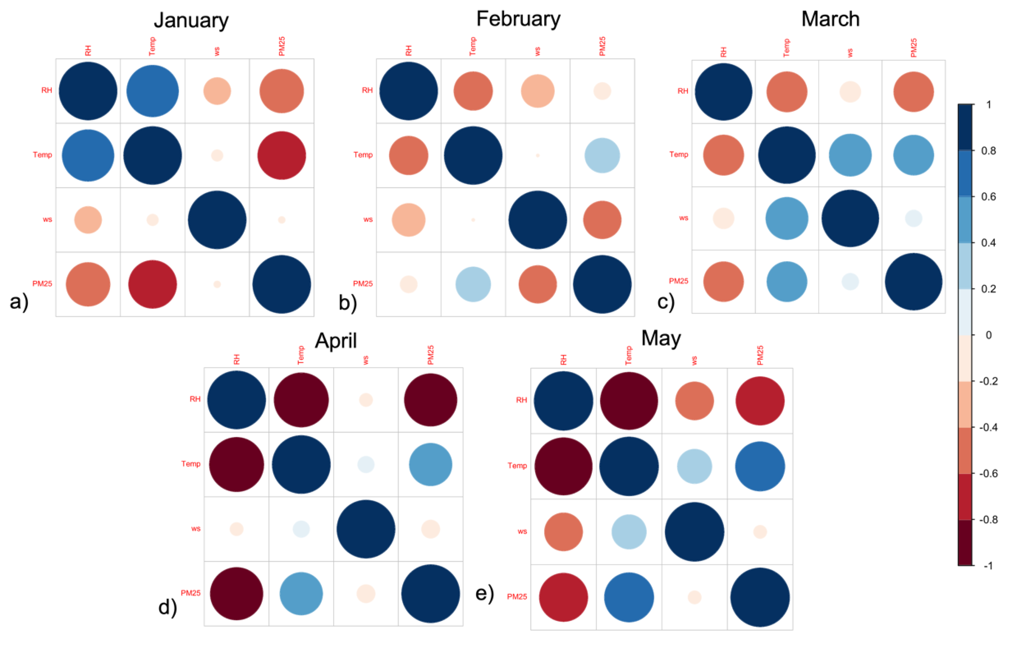
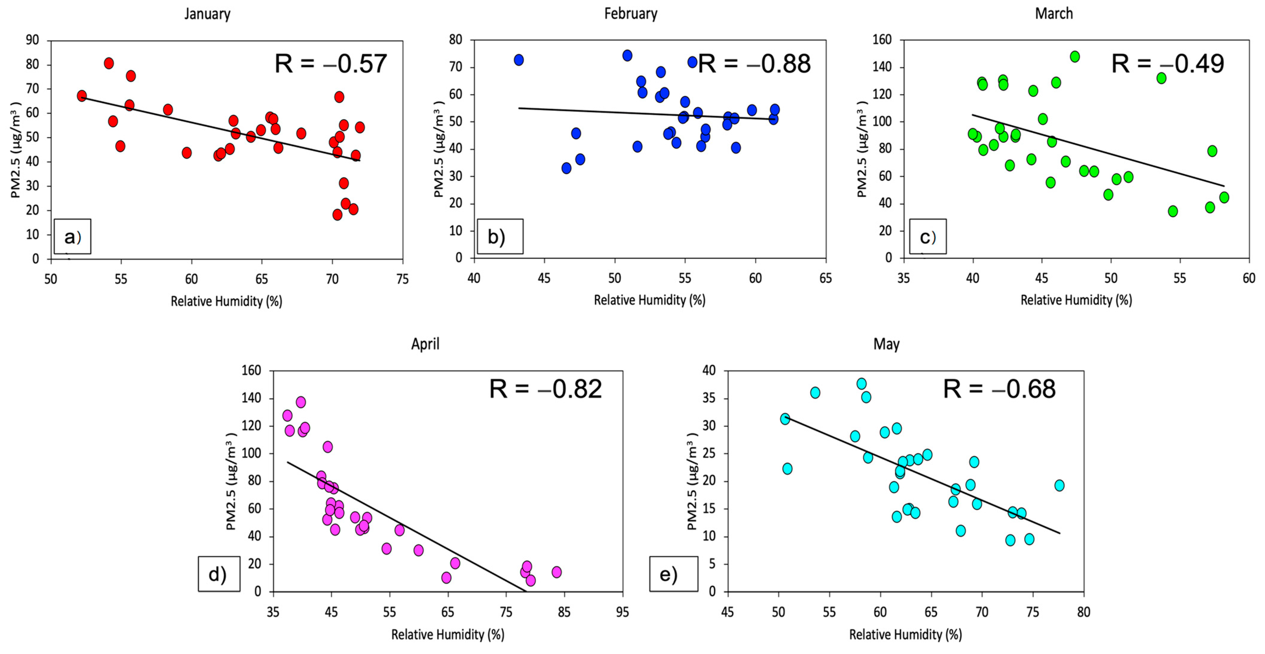
3.2. Correlation between PM2.5 and Meteorological Condition

Figure 3 shows the correlation between PM2.5 and meteorological variables including relative humidity (RH), surface temperature (Temp), and wind speed (ws) during January and May 2020 in northern Thailand. The PM2.5 concentration for all months was negatively related to relative humidity. Furthermore, a negative relationship was found between PM2.5 and temperature in January, while a positive relationship was found in the other months. The PM2.5 in most of the months was also negatively correlated with wind speed, while a negative relationship was found in March. The relationships of different air pollutants with wind speed and wind direction are illustrated in Figure 4. In general, dominant PM2.5 concentrations originate from the southeast (0–1 m·s−1). In March, high concentrations of PM2.5 (100 μg/m3 and above) originate from the southeast and west (0–0.8 m·s−1), while the lowest concentration was found with the same wind direction when wind speeds were low (0–0.5 m·s−1). These results reflect previous findings that high concentrations of PM2.5 were mostly associated with low wind speed conditions and when weak winds prevail along the southeast [33,34] (Shelton et al., 2022; Hama et al., 2020).
The linear regression analysis between PM2.5 and meteorological variables is also shown in Figure 5, Figure 6 and Figure 7. Figure 5 demonstrates a mainly negative relationship between wind speed and PM2.5 from January to May. These results are similar to previous studies, such as those by Wang and Ogawa [35], Ren et al. [36], and Sirithian et al. [37]. In general, the relative humidity and temperature were strongly correlated with the PM2.5 concentration; in contrast, the wind speed was slightly correlated with the PM2.5 concentration in northern Thailand. In cases where the wind speed is modest, pollutants could be blown away within a particular geographical area, but if the wind speed is strong, the huge amounts of pollutants could be transported from a long distance away. Between January and May, Figure 6 depicts the positive connection between temperature and PM2.5. This result is similar to findings observed by Zhang et al. [38] and Han et al. [39]. Except for January, when a high negative correlation is observed, PM2.5 shows a mostly strong positive relationship with temperature during the rest of the months. This is due to the fact that temperature influences particle formation; hence, a high temperature increases the photochemical reaction between precursors, whilst a low temperature might delay the process and contribute to PM2.5. The linear correlation between PM2.5 concentration and relative humidity is depicted in Figure 7. During most months, PM2.5 has a strong inverse relationship with relative humidity, similar to findings by Liu et al. [40]. Positive correlations were found in February, although the correlation coefficient is relatively low. When the humidity exceeds 70% in April and May, PM2.5 concentration shows a strong negative correlation with relative humidity. The Pearson correlation coefficient also highlights the relationships between PM2.5 and meteorological variables. There is a strong negative correlation between PM2.5 and relative humidity ranging between −0.88 and −0.49 and a weak correlation between PM2.5 and wind speed ranging between −0.096 and 0.087, as well as a positive correlation related to temperature ranging between 0.56 and 0.70. According to the findings, an increase in surface temperature and a reduction in relative humidity during the summer season had a significant impact on PM2.5 concentrations in northern Thailand.
In this study, there was a negative correlation between relative humidity and PM2.5. In general, relative humidity regulates particle movement and therefore can induce particulate matter to sink to the surface. As a result, if relative humidity increases, PM2.5 tends to decrease [41,42]. Moreover, airborne particles condense and become dense enough for both dry and wet deposition when relative humidity reaches the threshold, leading to much lower PM2.5 concentrations [39]. There is also a strong positive correlation between temperature and PM2.5. Since temperature affects particle production, a high temperature may enhance the photochemical reaction involving precursors [38]. The higher temperatures speed up photochemical reactions, which raise precursor levels of PM2.5 and other secondary pollutants as well as PM2.5 concentrations [43,44]. However, there was a negative correlation in January. This type of detrimental effect is mostly brought on by temperature-related air convections and losses of PM2.5. In addition, the negative relationship is likely due to high temperatures, which facilitate the air’s convection, which leads to the diluting and dispersal of PM2.5 [44]. Turbulence, which is caused by intense thermal activity at high temperatures, speeds up the distribution of PM2.5 [21,22]. In addition, because of the low surface temperature in the winter, warming might cause temperature inversion layers, which are unfavorable for airflow and may encourage the accumulation of PM2.5 [34]. The wind’s direction also has a significant impact on PM2.5 concentrations. The wind carries various amounts of contaminants in various directions [45]. In general, when the wind is blowing at a moderate speed, contaminants can be dispersed within a small geographic area, but when the wind is strong enough, it can carry significant amounts of pollutants over considerable distances [45]. Furthermore, wind speed influences pollution levels in many different geographic regions [46]. For example, it has less of an impact on pollution levels in clean environments, such as forests, mountains, or coastal areas, while it increases pollution levels in megacities and heavily industrialized areas [46].
In this study, the relationship between wind speed and PM2.5 is inverse. This is most likely the outcome of several factors. The circumstances for PM2.5 diffusion are mostly made perfect by an increase in wind speed, particularly a high wind speed [29]. Hence, increasing wind speed has a greater impact on removing PM2.5 concentrations from the atmosphere. Second, increased wind speed may result in larger evaporation losses and, thus, lower PM2.5 mass concentrations because wind speed is a key determinant in PM2.5 evaporation [30]. Wind speed may occasionally have a positive impact on PM2.5 concentrations. Initial increases in wind speed in light winds may result in low levels of turbulence, modest horizontal atmospheric movement, and a predominance of sinking movement in the upper air, creating unfavorable circumstances for PM2.5 and other pollutants to disperse [28,35].

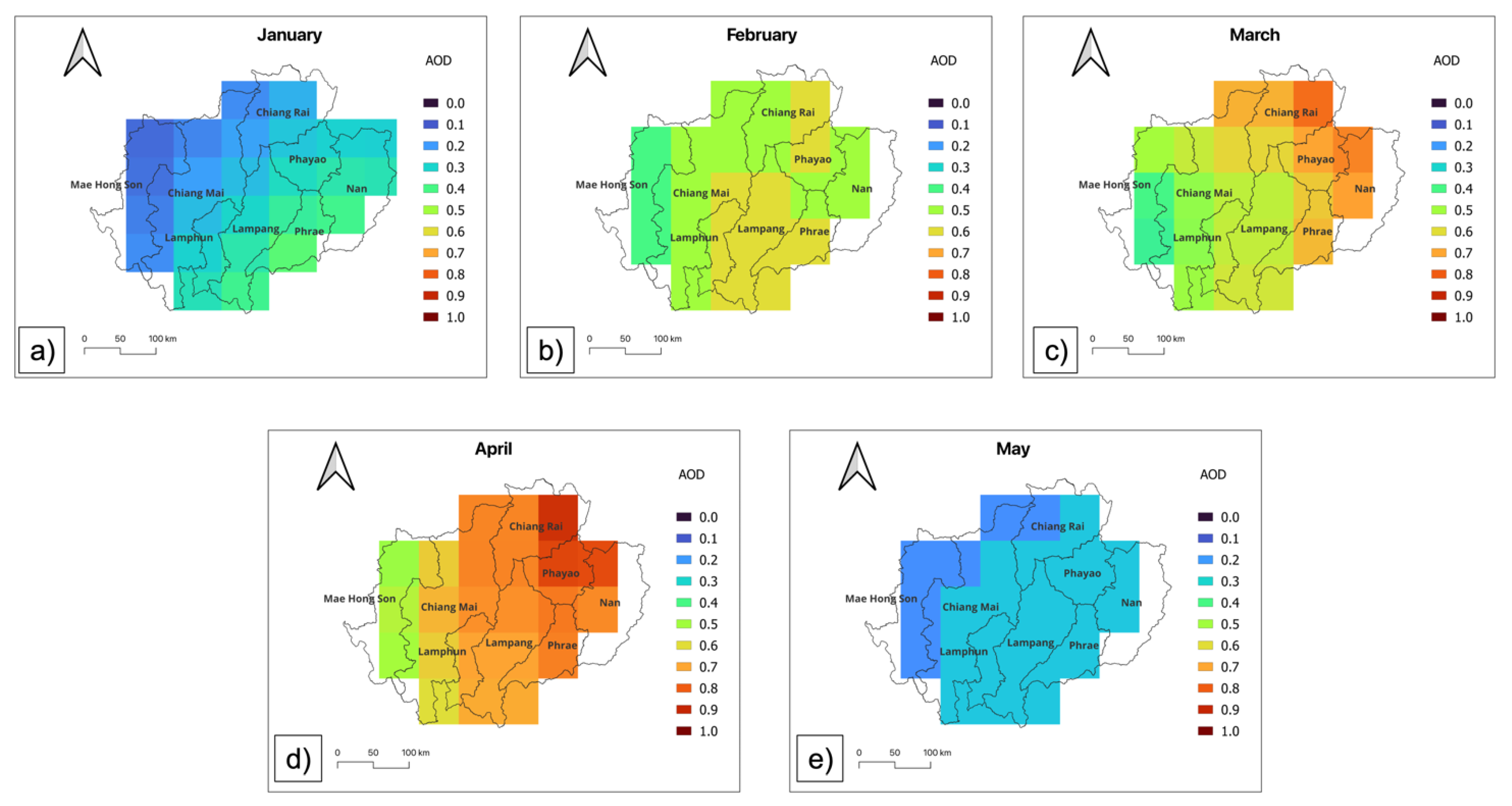
3.3. PM2.5, and Aerosol Optical Depth

Figure 8 and Figure 9 show the spatial distribution of PM2.5 (Figure 6) and aerosol optical depth (Figure 7). In general, the levels of PM2.5 concentrations were in the range of 16 to 195 µg/m3 from January to May 2020. In January, the highest distribution of PM2.5 concentrations was found in Lampang province, ranging from 150 to 195 µg/m3, while a range of 61 to 106 µg/m3 was found in the bulk of provinces. In February, the distribution of PM2.5 concentrations in Chiang Rai province reached 195 µg/m3 at the top of the area. At the same time, PM2.5 concentrations were in the range of 106–150 µg/m3 in the rest of northern Thailand. In March, the PM2.5 concentrations were lower than in February, excluding the upper part of Chiang Rai province. In April, the PM2.5 was more evenly distributed than it was in March in the entire region, with the concentration ranging from 106 to 195 µg/m3 in most of the region. In May, the PM2.5 concentrations were similar to April, except the highest concentration was found in Chiang Mai province. The results of AOD from MERRA in Figure 4 correspond to the PM2.5 concentration in Figure 3. AOD was generally in the range of 0.1 to 0.9 from January to April. In January, AOD was not too high for the whole region, while it tended to increase in February, reaching 0.6 in Lampang, Chiang Rai, and Phayao provinces. In March, AOD increased by 0.7 in many provinces, such as Chiang Rai, Phayao, Nan, and Phrae. In April, AOD was extremely high in most areas including Chiang Rai, Phayao, Nan, Phrae, Lampang, and Chiang Mai, ranging from 0.7 to 0.9.
There are numerous similarities between PM2.5 and AOD, despite the fact that their association is not always reliable [47,48]. While AOD represents the entire atmospheric column, PM2.5 primarily represents the atmospheric turbidity near the surface. Additionally, because PM2.5 primarily represents the concentration of dry mass of fine particles, which is barely influenced by coarse particles and water vapor, the AOD also takes into account the influence of these two factors. According to this study, the AOD pattern in northern Thailand and the PM2.5 concentration are most likely related. The similar pattern between PM2.5 and AODs is most likely caused by the variations in aerosol type and properties in this region according to Yang et al. [49], who examined the relationships between PM2.5 and AOD in 368 Chinese cities from February 2013 to December 2017 at various temporal and regional scales. In their study, urban regions, which are similar to the study area in this paper, also showed a strong association between PM2.5 and AOD.

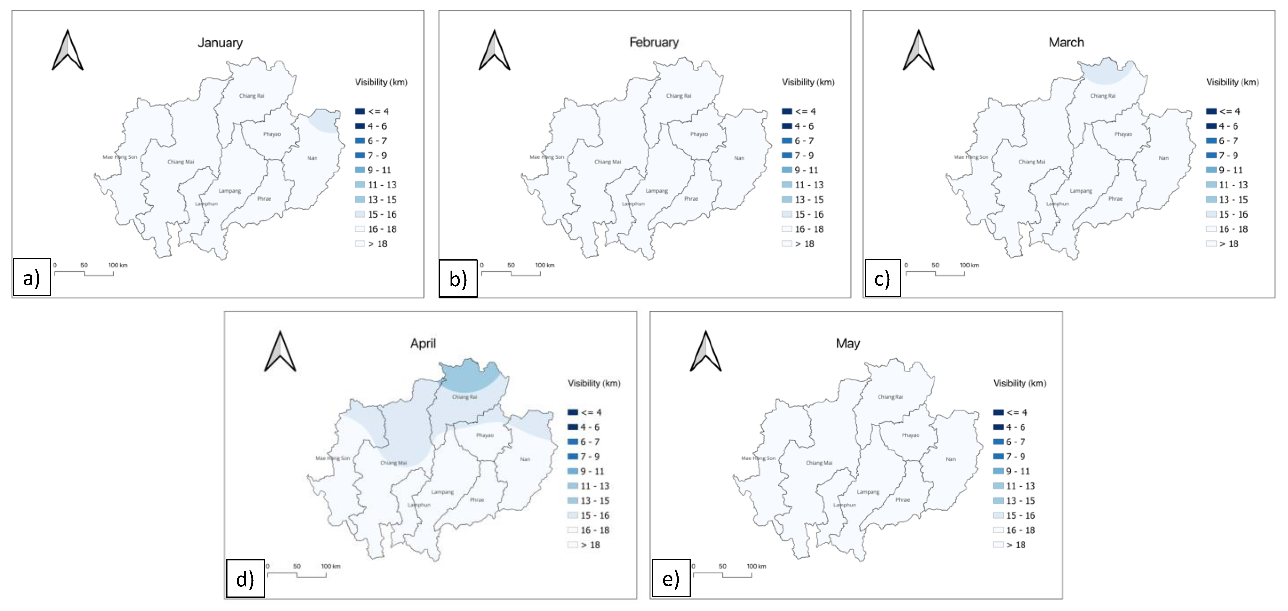
3.4. Fire, Plume, and Visibility

The smoke plume and fire in the months of January, February, March, April, and May 2020 are shown in the images from NASA satellites taken by the Moderate Resolution Integrated Aging Spectroradiometer (MODIS). The massive plumes of smoke were seen billowing across the majority of northern Thailand. No rain clouds are expected to arrive to put an end to the burning and smoke that are engulfing the area. Furthermore, from January to May, images of multiple fires growing in northern Thailand were captured by the NOAA/NASA Suomi NPP and NOAA 20 satellites (Figure 10). The area appears to be completely aflame (Figure 11). Agricultural burning is the most likely reason for the fires in this region [3]. It is likely due to the farmers burning their fields to prepare for the new planting season in Southeast Asia at this time of year.
Figure 12, Figure 13 and Figure 14 show the spatial distribution of visibility in northern Thailand in 2020. At mixing height level at 1 km above ground level, low visibility generally occurred in March and April by <4 km at Chiang Rai province in March (Figure 12c), and in the range of 4–6 km in many areas of upper northern Thailand (Figure 12d) in April, while there was very clear visibility in May (Figure 12e). In January, the visibility was very clear, ranging between 13 and 18 km, while it was reduced to 6− < 4 km during February and April. In general, at the mixing height level of 1.5 km above ground level, the visibility is clearer than at 1.0 km, and the lowest visibility was also found in the range of 7–9 km in March and April in Chiang Rai province. The visibility was very clear in January and May with a value of 15–18 km; during February to April there was lower visibility. At the mixing height level of 3 km, the visibility was mostly clear compared to other levels ranging from 11–18 km for all months.
In comparison to the very clear visibility in May, during the haze months (January to April), PM2.5 tends to reduce visibility for all provinces (Figure 15). PM2.5 potentially reduces visibility in the range of 20–70%, 60–80%, 60–90%, and 70–90% in January, February, March, and April 2020 for all provinces. Massive fires in both domestic areas and areas surrounding northern Thailand from January to April contribute to huge amounts of smoke that cause low visibility in northern Thailand, especially at 1 km above ground level, with reduced visibility in the range of 70–90% for all provinces in April. As displayed in Table 2, during the haze episode (January to April), a 1 μg/m3 increase in PM2.5 essentially reduced visibility 0.30 ± 0.05, 0.83 ± 0.33, 0.32 ± 0.07, 0.48 ± 0.05, and 0.31 ± 0.04 in Chiang Mai, Chiang Rai, Lampang, Lamphun, and Nan provinces, respectively. At the same time, it was associated with a visibility reduction in range of 0.18–0.35 km, 0.20–1.74 km, 0.13–0.42 km, 0.34–0.56 km, and 0.23–0.42 km in Chiang Mai, Chiang Rai, Lampang, Lamphun, and Nan provinces, respectively.
The results of this demonstrate that the high level of PM2.5 is likely to be the primary cause of the reduction of visibility in northern Thailand, which is similar to findings by Zhao et al. [50] and Sloane et al. [51]. Although there are other elements that affect atmospheric visibility besides ambient air pollution, meteorological parameters, particularly humidity, have a substantial direct and indirect impact on visibility degradation [52]. However, fine particulate matter is the main pollutant in most urban areas [53,54], and its detrimental effects on visibility have drawn attention all over the world [55]. While the haze event in northern Thailand takes place during the dry season with very low relative humidity ranging from 30 to 60% (Figure 5b), PM2.5 is the primary reason for the area’s poor visibility.

3.5. Air Pollution Mitigation

It is evident that air pollution is a regional problem in Southeast Asia. Since air has no boundaries, only regional cooperation can address the issue of air pollution [56]. Although most countries in Southeast Asia (SEA) are aware of the difficulties caused by transboundary air pollution, no long-lasting solutions have been found [57]. Transboundary international environmental law is desperately needed to prevent the polluting countries from further deterioration. The ASEAN Agreement on Transboundary Haze Pollution (AATHP), a legally enforceable regional agreement, was established to tackle the haze issue in SEA [58]. The AATHP, however, is usually seen as a failure [59,60]. Reaching a regional agreement on the issue of atmospheric pollution has proven challenging due to uncertainties surrounding the identification of pollutant sources’ locations [61,62].
Although there are several ways to identify transboundary air pollution, none are commonly used. Determining transboundary air pollution requires an understanding of the relationships between pollution emissions and the types, amounts, and consequences of depositions in receiving areas [63]. The issue of transboundary air pollution may be resolved by better knowledge of the scientific understanding of the source–receptor interaction in this region [64]. Insufficient in situ sampling and measurement of air pollutants, uncertainty in space-borne observation, and an inadequate emission inventory analysis (EIA) in the area are a few of the concerns that need to be addressed. The foundation of satellite remote sensing and numerical modeling approaches to determine transboundary air pollution is in situ sampling and measurements. The density and distribution of monitoring sites over SEA has not been adequate. Local administrations that run monitoring stations are present in just seven out of the ten ASEAN nations. In less economically developed nations, poor levels of maintenance at existing monitoring stations are another issue. Moreover, one of the primary causes of air pollution in the Indochina peninsula is biomass burning [65]. The three countries with the most fires in this region are Burma, Cambodia, and Laos, according to satellite-borne measurements [66]. The results of the contributions to transboundary air pollution from various geographic sources provide some information for policymaking.
Moreover, because fire from forests is a huge contributory source of smoke plume in SEA, forest fuel management is recommended for policymakers [67]. Prescribed burning is the best strategy for controlling forest fires in many nations. For example, during the dry season, a significant amount of leaf litter is produced by the forest, particularly in the north and west of Thailand. Specific parts may need to be incinerated for disposal, which must be performed at the proper time and location [67]. This will lessen smog brought on by out-of-control forest fires, preserve the health of the forest, and lessen damage from forest fires. Despite the fact that there are ongoing efforts to reduce, recycle, and utilize forest leftovers and large forest regions are always protected with fire barriers, it is challenging to maintain and govern huge forests. A zero-burning policy can reportedly reduce open burning activities in northern Thailand, according to Yabueng et al. [68]. Although biomass fires’ fine particle levels have decreased, there are still extensive areas of smoke haze. The PM2.5 fraction reduced during the period when the policy for prohibiting open fires was extended from two months (middle of February through middle of April) to around three months (middle of February through middle of May). Hence, while the regulation is being implemented, open burning incidents can be decreased. According to the description above, particulate matter, which contributes to several air pollution issues, is often generated by biomass or lignocellulosic biomass waste. However, this substance might be turned into high-value goods, such as biomaterials, biochemicals, and fuels [69]. This process of valuing could also reduce the CO2 and PM emissions brought on by the direct burning of a significant volume of biomass, which causes air pollution.
These initiatives are impossible to carry out without regional collaboration and the political will to push forward policies that aim to address poor air quality. Due to these considerations, tackling problems might be just as political or environmental. Governments in the area will need to make long-term financial and political commitments to pollution monitoring and research, as well as to sharing information and effectively responding to evidence of chronically poor air quality, in order to meet this challenge. For administrators of the environment and decision makers in charge of making policies at the municipal, national, and regional levels, this study could potentially offer information that is essential. Without solid recommendations and counsel based on scientific knowledge and competence, decision making cannot be accomplished effectively. This is also true of diplomatic efforts to reduce air pollution in this region that are successful and efficient.

3.6. Limitation of the Study

Linear regression cannot adequately describe the relationship between PM2.5 and meteorological variables because these interactions are rarely linear in real environments. For instance, various mechanisms explain how meteorological conditions influence the accumulation and dispersion of PM2.5 [70]. Meteorological conditions and PM2.5 levels both influence the complicated relationships between PM2.5 and meteorology [71]. As a result, there are noticeable characteristics of meteorological influences on PM2.5 concentrations due to considerable fluctuations in meteorological circumstances and PM2.5 concentrations. For linearly separable data, however, linear regression performs remarkably well. Furthermore, it is simpler to use and understand and effective for explanation.

4. Conclusions

This study aims to investigate the distribution of PM2.5 and how meteorological conditions control its accumulation, as well as the effect of PM2.5 on visibility in northern Thailand in 2020. Several datasets were used in this study, including ground-based measurements from the Pollution Control Department in northern Thailand, aerosol optical depth (AOD) data from Modern-Era Retrospective Analysis for Research and Applications version 2 (MERRA-2), and satellite images from VIIRS S-NPP CORRECTED REFLECTANCE (TRUE COLOR) and VIIRS NOAA-20. The spatial distribution was utilized by GIS analysis. The daily average of PM2.5 concentrations exceeded both Thailand’s and the USEPA’s standards, especially from January to May. The highest values of PM2.5 concentrations were reported between 150 and 195 µg/m3 from March to April. The favorable weather conditions induced the accumulation of PM2.5 in northern Thailand. PM2.5 had a negative association with both wind speed and relative humidity, although it had a positive correlation with temperature. The high PM2.5 values in northern Thailand were caused by favorable climatic conditions. Because of the high concentration of PM2.5, AOD ranged from 0.1 to 0.9 from January to April. AODs ranging from 0.7 to 0.9 have been recorded in Chiang Rai, Phayao, Nan, Phrae, Lampang, and Chiang Mai provinces, particularly in March and April. Between January and April, a massive fire from both domestic sources and neighboring countries contributed to huge plumes of smoke that were a long-range transport of pollutants to Thailand. As a result, visibility was reduced by up to 90% when compared to normal conditions.

Author Contributions

Conceptualization, T.A.; methodology, P.K., P.P. and T.A.; software, T.A.; validation, T.A.; formal analysis, T.A.; investigation, P.K., P.P. and T.A.; resources, T.A.; data curation, P.K., P.P. and T.A; writing—original draft preparation, T.A.; writing—review and editing, T.A.; visualization, T.A.; supervision, T.A.; project administration, T.A.; funding acquisition, T.A. All authors have read and agreed to the published version of the manuscript.

Funding

This research was funded by University of Phayao and the APC was funded by University of Phayao.

Data Availability Statement

The data presented in this study are available in this article.

Acknowledgments

We would like to thank the Pollution Control Department from Thailand for supporting ground-based measurement data.

Conflicts of Interest

The authors declare no conflict of interest.

References

  1. Chen, J.; Li, Z.; Lv, M.; Wang, Y.; Wang, W.; Zhang, Y.; Wang, H.; Yan, X.; Sun, Y.; Cribb, M. Aerosol hygroscopic growth, contributing factors, and impact on haze events in a severely polluted region in northern China. Atmos. Chem. Phys. 2019, 19, 1327–1342. [Google Scholar] [CrossRef] [Green Version]
  2. Wang, X.; Fu, T.M.; Zhang, L.; Lu, X.; Liu, X.; Amnuaylojaroen, T.; Latif, M.T.; Ma, Y.; Zhang, L.; Feng, X.; et al. Rapidly changing emissions drove substantial surface and tropospheric ozone increases over Southeast Asia. Geo. Res. Lett. 2022, 49, e2022GL100223. [Google Scholar] [CrossRef]
  3. Amnuaylojaroen, T.; Inkom, J.; Janta, R.; Surapipith, V. Long range transport of southeast asian PM2.5 pollution to northern Thailand during high biomass burning episodes. Sustainability 2020, 12, 10049. [Google Scholar] [CrossRef]
  4. Huang, W.-R.; Wang, S.-H.; Yen, M.-C.; Lin, N.-H.; Promchote, P. Interannual variation of springtime biomass burning in Indochina: Regional differences, associated atmospheric dynamical changes, and downwind impacts. J. Geophys. Res. Atmos. 2016, 121, 10016–10028. [Google Scholar] [CrossRef] [PubMed]
  5. Yin, S.; Wang, X.; Zhang, X.; Guo, M.; Miura, M.; Xiao, Y. Influence of biomass burning on local air pollution in mainland Southeast Asia from 2001 to 2016. Environ. Pollut. 2019, 254, 112949. [Google Scholar] [CrossRef]
  6. Amnuaylojaroen, T.; Barth, M.; Emmons, L.; Carmichael, G.; Kreasuwun, J.; Prasitwattanaseree, S.; Chantara, S. Effect of different emission inventories on modeled ozone and carbon monoxide in Southeast Asia. Atmos. Chem. Phys. 2014, 14, 12983–13012. [Google Scholar] [CrossRef] [Green Version]
  7. Lee, H.-H.; Iraqui, O.; Gu, Y.; Yim, S.H.-L.; Chulakadabba, A.; Tonks, A.Y.-M.; Yang, Z.; Wang, C. Impacts of air pollutants from fire and non-fire emissions on the regional air quality in Southeast Asia. Atmos. Chem. Phys. 2018, 18, 6141–6156. [Google Scholar] [CrossRef] [Green Version]
  8. Amnuaylojaroen, T.; Kreasuwun, J. Investigation of fine and coarse particulate matter from burning areas in Chiang Mai, Thailand using the WRF/CALPUFF. Chiang Mai J. Sci. 2012, 39, 311–326. [Google Scholar]
  9. Khodmanee, S.; Amnuaylojaroen, T. Impact of Biomass Burning on Ozone, Carbon Monoxide, and Nitrogen Dioxide in Northern Thailand. Front. Environ. Sci. 2021, 9, 27. [Google Scholar] [CrossRef]
  10. He, H.; Tie, X.; Zhang, Q.; Liu, X.; Gao, Q.; Li, X.; Gao, Y. Analysis of the causes of heavy aerosol pollution in Beijing, China: A case study with the WRF-Chem model. Particuology 2015, 20, 32–40. [Google Scholar] [CrossRef]
  11. Pohjola, M.A.; Kousa, A.; Kukkonen, J.; Härkönen, J.; Karppinen, A.; Aarnio, P.; Koskentalo, T. The spatial and temporal variation of measured urban PM10 and PM2.5 in the Helsinki metropolitan area. Water Air Soil Pollut. Focus 2002, 2, 189–201. [Google Scholar] [CrossRef]
  12. Tai, A.P.; Mickley, L.J.; Jacob, D.J. Correlations between fine particulate matter (PM2. 5) and meteorological variables in the United States: Implications for the sensitivity of PM2.5 to climate change. Atmos. Environ. 2010, 44, 3976–3984. [Google Scholar] [CrossRef]
  13. Akbal, Y.; Ünlü, K.D. A deep learning approach to model daily particular matter of Ankara: Key features and forecasting. Int. J. Environ. Sci. Technol. 2021, 19, 5911–5927. [Google Scholar] [CrossRef]
  14. Shahriar, S.A.; Kayes, I.; Hasan, K.; Salam, M.A.; Chowdhury, S. Applicability of machine learning in modeling of atmospheric particle pollution in Bangladesh. Air Qual. Atmos. Health 2020, 13, 1247–1256. [Google Scholar] [CrossRef] [PubMed]
  15. Franceschi, F.; Cobo, M.; Figueredo, M. Discovering relationships and forecasting PM10 and PM2.5 concentrations in Bogotá, Colombia, using artificial neural networks, principal component analysis, and k-means clustering. Atmos. Pollut. Res. 2018, 9, 912–922. [Google Scholar] [CrossRef]
  16. Feng, X.; Li, Q.; Zhu, Y.; Hou, J.; Jin, L.; Wang, J. Artificial neural networks forecasting of PM2.5 pollution using air mass trajectory based geographic model and wavelet transformation. Atmos. Environ. 2015, 107, 118–128. [Google Scholar] [CrossRef]
  17. Akdi, Y.; Okkaoğlu, Y.; Gölveren, E.; Yücel, M.E. Estimation and forecasting of PM 10 air pollution in Ankara via time series and harmonic regressions. Int. J. Environ. Sci. Technol. 2020, 17, 3677–3690. [Google Scholar] [CrossRef] [Green Version]
  18. Zhao, J.; Kong, X.; He, K.; Xu, H.; Mu, J. Assessment of the radiation effect of aerosols on maize production in China. Sci. Total Environ. 2020, 720, 137567. [Google Scholar] [CrossRef]
  19. Wei, K.; Tang, X.; Tang, G.; Wang, J.; Xu, L.; Li, J.; Ni, C.; Zhou, Y.; Ding, Y.; Liu, W. Distinction of two kinds of haze. Atmos. Environ. 2020, 223, 117228. [Google Scholar] [CrossRef]
  20. Zeng, W.; Liu, T.; Du, Q.; Li, J.; Xiao, J.; Guo, L.; Li, X.; Xu, Y.; Xu, X.; Wan, D.; et al. The interplay of haze characteristics on mortality in the Pearl River Delta of China. Environ. Res. 2020, 184, 109279. [Google Scholar] [CrossRef]
  21. Yang, X.; Zhao, C.; Guo, J.; Wang, Y. Intensification of aerosol pollution associated with its feedback with surface solar radiation and winds in Beijing. J. Geophys. Res. Atmos. 2016, 121, 4093–4099. [Google Scholar] [CrossRef]
  22. Yang, X.; Zhao, C.; Zhou, L.; Wang, Y.; Liu, X. Distinct impact of different types of aerosols on surface solar radiation in China. J. Geophys. Res. Atmos. 2016, 121, 6459–6471. [Google Scholar] [CrossRef]
  23. Zhang, X.; Zhang, Q.; Hong, C.; Zheng, Y.; Geng, G.; Tong, D.; Zhang, Y.; Zhang, X. Enhancement of PM2.5 concentrations by aerosol-meteorology interactions over China. J. Geophys. Res. Atmos. 2018, 123, 1179–1194. [Google Scholar] [CrossRef]
  24. Liu, F.; Fang, P.; Yao, Z.; Fan, R.; Pan, Z.; Sheng, W.; Yang, H. Recovering 6D object pose from RGB indoor image based on two-stage detection network with multi-task loss. Neurocomputing 2019, 337, 15–23. [Google Scholar] [CrossRef]
  25. Guan, L.; Liang, Y.; Tian, Y.; Yang, Z.; Sun, Y.; Feng, Y. Quantitatively analyzing effects of meteorology and PM2.5 sources on low visual distance. Sci. Total Environ. 2019, 659, 764–772. [Google Scholar] [CrossRef] [PubMed]
  26. Wong, C.-M.; Vichit-Vadakan, N.; Kan, H.; Qian, Z. Public Health and Air Pollution in Asia (PAPA): A multicity study of short-term effects of air pollution on mortality. Environ. Health Perspect. 2008, 116, 1195–1202. [Google Scholar] [CrossRef] [PubMed] [Green Version]
  27. Amnuaylojaroen, T. Prediction of PM2.5 in an urban area of northern Thailand using multivariate linear regression model. Adv. Meteorol. 2022, 2022, 3190484. [Google Scholar] [CrossRef]
  28. Bedient, P.B.; Huber, W.C.; Vieux, B.E. Hydrology and Floodplain Analysis; Prentice Hall: Upper Saddle River, NJ, USA, 2008; Volume 816. [Google Scholar]
  29. Burrough, P.A.; McDonnell, R.A.; Lloyd, C.D. Principles of Geographical Information Systems; Oxford University Press: Oxford, UK, 2015. [Google Scholar]
  30. Bäumer, D.; Vogel, B.; Versick, S.; Rinke, R.; Möhler, O.; Schnaiter, M. Relationship of visibility, aerosol optical thickness and aerosol size distribution in an ageing air mass over South-West Germany. Atmos. Environ. 2008, 42, 989–998. [Google Scholar] [CrossRef]
  31. Carabali, G.; Villanueva-Macias, J.; Ladino, L.A.; Álvarez-Ospina, H.; Raga, G.B.; Andraca-Ayala, G.; Miranda, J.; Grutter, M.; Silva, M.M.; Riveros-Rosas, D. Characterization of aerosol particles during a high pollution episode over Mexico City. Sci. Rep. 2021, 11, 22533. [Google Scholar] [CrossRef]
  32. Amnuaylojaroen, T.; Macatangay, R.C.; Khodmanee, S. Modeling the effect of VOCs from biomass burning emissions on ozone pollution in upper Southeast Asia. Heliyon 2019, 5, e02661. [Google Scholar] [CrossRef] [Green Version]
  33. Hama, S.M.; Kumar, P.; Harrison, R.M.; Bloss, W.J.; Khare, M.; Mishra, S.; Namdeo, A.; Sokhi, R.; Goodman, P.; Sharma, C. Four-year assessment of ambient particulate matter and trace gases in the Delhi-NCR region of India. Sustain. Cities Soc. 2020, 54, 102003. [Google Scholar] [CrossRef]
  34. Shelton, S.; Liyanage, G.; Jayasekara, S.; Pushpawela, B.; Rathnayake, U.; Jayasundara, A.; Jayasooriya, L.D. Seasonal Variability of Air Pollutants and Their Relationships to Meteorological Parameters in an Urban Environment. Adv. Meteorol. 2022, 2022, 5628911. [Google Scholar] [CrossRef]
  35. Wang, J.; Ogawa, S. Effects of meteorological conditions on PM2.5 concentrations in Nagasaki, Japan. Int. J. Environ. Res. Public Health 2015, 12, 9089–9101. [Google Scholar] [CrossRef] [PubMed]
  36. Ren, J.; Liu, J.; Li, F.; Cao, X.; Ren, S.; Xu, B.; Zhu, Y. A study of ambient fine particles at Tianjin International Airport, China. Sci. Total Environ. 2016, 556, 126–135. [Google Scholar] [CrossRef]
  37. Sirithian, D.; Thanatrakolsri, P. Relationships between Meteorological and Particulate Matter Concentrations (PM2.5 and PM10) during the Haze Period in Urban and Rural Areas, Northern Thailand. Air Soil Water Res. 2022, 15, 1–15. [Google Scholar] [CrossRef]
  38. Zhang, Z.; Gong, D.; Mao, R.; Kim, S.-J.; Xu, J.; Zhao, X.; Ma, Z. Cause and predictability for the severe haze pollution in downtown Beijing in November–December 2015. Sci. Total Environ. 2017, 592, 627–638. [Google Scholar] [CrossRef]
  39. Han, J.; Wang, J.; Zhao, Y.; Wang, Q.; Zhang, B.; Li, H.; Zhai, J. Spatio-temporal variation of potential evapotranspiration and climatic drivers in the Jing-Jin-Ji region, North China. Agric. For. Meteorol. 2018, 256, 75–83. [Google Scholar] [CrossRef]
  40. Liu, P.F.; Zhao, C.S.; Gbel, T.; Hallbauer, E.; Nowak, A.; Ran, L.; Xu, W.Y.; Deng, Z.Z.; Ma, N.; Mildenberger, K.; et al. Hygroscopic properties of aerosol particles at high relative humidity and their diurnal variations in the north china plain. Atmos. Chem. Phys. 2011, 11, 3479–3794. [Google Scholar] [CrossRef] [Green Version]
  41. Giri, D.; Adhikary, P.R.; Murthy, V.K. The influence of meteorological conditions on PM10 concentrations in Kathmandu Valley. Int. J. Environ. Res. 2008, 2, 49–60. [Google Scholar]
  42. Kayes, I.; Shahriar, S.A.; Hasan, K.; Akhter, M.; Kabir, M.M.; Salam, M.A. The relationships between meteorological parameters and air pollutants in an urban environment. Glob. J. Environ. Sci. Manag. 2019, 5, 265–278. [Google Scholar] [CrossRef]
  43. Luo, J.; Du, P.; Samat, A.; Xia, J.; Che, M.; Xue, Z. Spatiotemporal Pattern of PM2.5 Concentrations in Mainland China and Analysis of Its Influencing Factors using Geographically Weighted Regression. Sci. Rep. 2017, 7, 40607. [Google Scholar] [CrossRef] [PubMed] [Green Version]
  44. Zhang, C.; Ni, Z.; Ni, L. Multifractal detrended cross-correlation analysis between PM2.5 and meteorological factors. Phys. A Stat. Mech. Its Appl. 2015, 438, 114–123. [Google Scholar] [CrossRef]
  45. Wang, M.; Cao, C.; Li, G.; Singh, R.P. Analysis of a severe prolonged regional haze episode in the Yangtze River Delta, China. Atmos. Environ. 2015, 102, 112–121. [Google Scholar] [CrossRef]
  46. Pushpawela, B.; Jayaratne, R.; Morawska, L. The influence of wind speed on new particle formation events in an urban environment. Atmos. Res. 2019, 1, 37–41. [Google Scholar] [CrossRef]
  47. Zhang, Y.; Li, Z. Remote sensing of atmospheric fine particulate matter (PM2.5) mass concentration near the ground from satellite observation. Remote Sens. Environ. 2015, 160, 252–262. [Google Scholar] [CrossRef]
  48. Zheng, C.; Zhao, C.; Zhu, Y.; Wang, Y.; Shi, X.; Wu, X.; Chen, T.; Wu, F.; Qiu, Y. Analysis of influential factors for the relationship between PM2.5 and AOD in Beijing. Atmos. Chem. Phys. 2017, 17, 13473–13489. [Google Scholar] [CrossRef] [Green Version]
  49. Yang, Q.; Yuan, Q.; Li, T.; Shen, H.; Zhang, L. The relationships between PM2.5 and meteorological factors in China: Seasonal and regional variations. Int. J. Environ. Res. Public Health 2017, 14, 1510. [Google Scholar] [CrossRef] [Green Version]
  50. Zhao, X.J.; Zhang, X.L.; Xu, X.F.; Xu, J.; Meng, W.; Pu, W.W. Seasonal and diurnal variations of ambient PM2.5 concentration in urban and rural environments in Beijing. Atmos. Environ. 2009, 43, 2893–2900. [Google Scholar] [CrossRef]
  51. Sloane, C.S.; Watson, J.; Chow, J.; Pritchett, L.; Willard Richards, L. Size–segregated fine particle measurements by chemical species and their impact on visibility impairment in Denver. Atmos. Environ. Part A Gen. Top. 1991, 25, 1013–1024. [Google Scholar] [CrossRef]
  52. Yang, Z.; Wang, Y.; Xu, X.H.; Yang, J.; Ou, C.Q. Quantifying and characterizing the impacts of PM2.5 and humidity on atmospheric visibility in 182 Chinese cities: A nationwide time-series study. J. Clean. Prod. 2022, 368, 133182. [Google Scholar] [CrossRef]
  53. Zhang, H.; Hoff, R.M.; Engel-Cox, J.A. The relation between Moderate Resolution Imaging Spectroradiometer (MODIS) aerosol optical depth and PM2.5 over the United States: A geographical comparison by US Environmental Protection Agency regions. J. Air Waste Manag. Assoc. 2009, 59, 1358–1369. [Google Scholar] [CrossRef] [PubMed] [Green Version]
  54. Zhang, Q.; Streets, D.G.; Carmichael, G.R.; He, K.B.; Huo, H.; Kannari, A.; Klimont, Z.; Park, I.S.; Reddy, S.; Fu, J.S.; et al. Asian emissions in 2006 for the NASA INTEX–B mission. Atmos. Chem. Phys. 2009, 9, 5131–5153. [Google Scholar] [CrossRef] [Green Version]
  55. Aouizerats, B.; Van Der Werf, G.R.; Balasubramanian, R.; Betha, R. Importance of transboundary transport of biomass burning emissions to regional air quality in Southeast Asia during a high fire event. Atmos. Chem. Phys. 2015, 15, 363–373. [Google Scholar] [CrossRef] [Green Version]
  56. Jones, D.S. ASEAN and transboundary haze pollution in Southeast Asia. Asia Eur. J. 2006, 4, 431–446. [Google Scholar] [CrossRef]
  57. ASEAN Cooperation on Environment. Indonesia Deposits Instrument of Ratification of the ASEAN Agreement on Transboundary Haze Pollution. 2015. Available online: https://environment.asean.org/indonesia-deposits-instrument-of-ratification-of-the-asean-agreement-on-transboundary-haze-pollution/ (accessed on 9 March 2023).
  58. Forsyth, T. Public concerns about transboundary haze: A comparison of Indonesia, Singapore, and Malaysia. Global Environ. Chang. 2014, 25, 76–86. [Google Scholar] [CrossRef] [Green Version]
  59. Nurhidayah, L.; Lipman, Z.; Alam, S. Regional environmental governance: An evaluation of the ASEAN legal framework for addressing transboundary haze pollution. Aust. J. Asian Law 2014, 15, 87. [Google Scholar]
  60. Hook, G.D.; Mason, R.; O’Shea, P. Regional Risk and Security in Japan: Whither the Everyday; Taylor & Francis: Abingdon, UK, 2015. [Google Scholar]
  61. Nobuhiko, S. We Cannot Afford to See PM2.5 Pollution Indifferently. Global Forum of Japan Commentary. Available online: http://www.gfj.jp/e/commentary/130426.pdf (accessed on 6 March 2023).
  62. Venkatram, A.; Karamchandani, P. Source-receptor relationships. A look at acid deposition modeling. Environ. Sci. Technol. 1986, 20, 1084–1091. [Google Scholar] [CrossRef]
  63. Chen, Q.; Taylor, D. Transboundary atmospheric pollution in Southeast Asia: Current methods, limitations and future developments. Crit. Rev. Environ. Sci. Technol. 2018, 48, 997. [Google Scholar] [CrossRef]
  64. Yadav, I.C.; Devi, N.L.; Li, J.; Syed, J.H.; Zhang, G.; Watanabe, H. Biomass burning in Indo-China peninsula and its impacts on regional air quality and global climate change: A review. Environ. Pollut. 2017, 227, 414–427. [Google Scholar] [CrossRef]
  65. Vadrevu, K.P.; Justice, C. Vegetation fires in the Asian region: Satellite observational needs and priorities. Global Environ. Res. 2011, 15, 65–76. [Google Scholar]
  66. Suriyawong, P.; Chuetor, S.; Samae, H.; Piriyakarnsakul, S.; Amin, M.; Furuuchi, M.; Hata, M.; Inerb, M.; Phairuang, W. Airborne particulate matter from biomass burning in Thailand: Recent issues, challenges, and options. Heliyon 2023, 9, e14261. [Google Scholar] [CrossRef]
  67. Chernkhunthod, C.; Hioki, Y. Fuel characteristics and fire behavior in mixed deciduous forest areas with different fire frequencies in Doi Suthep-Pui National Park, Northern Thailand. Landsc. Ecol. Eng. 2020, 16, 289–297. [Google Scholar] [CrossRef]
  68. Yabueng, N.; Wiriya, W.; Chantara, S. Influence of zero-burning policy and climate phenomena on ambient PM2.5 patterns and PAHs inhalation cancer risk during episodes of smoke haze in Northern Thailand. Atmos. Environ. 2020, 232, 117485. [Google Scholar] [CrossRef]
  69. Areepak, C.; Jiradechakorn, T.; Chuetor, S.; Phalakornkule, C.; Sriariyanun, M.; Raita, M.; Champreda, V.; Laosiripojana, N. Improvement of lignocellulosic pretreatment efficiency by combined chemo—Mechanical pretreatment for energy consumption reduction and biofuel production. Renew. Energy 2022, 182, 1094–1102. [Google Scholar] [CrossRef]
  70. Chen, Z.; Chen, D.; Zhao, C.; Kwan, M.P.; Cai, J.; Zhuang, Y.; Zhao, B.; Wang, X.; Chen, B.; Yang, J.; et al. Influence of meteorological conditions on PM2.5 concentrations across China: A review of methodology and mechanism. Environ. Int. 2020, 139, 105558. [Google Scholar] [CrossRef]
  71. Chen, Z.; Xie, X.; Cai, J.; Chen, D.; Gao, B.; He, B.; Cheng, N.; Xu, B. Understanding meteorological influences on PM2.5 concentrations across China: A temporal and spatial perspective. Atmos. Chem. Phys. 2018, 18, 5343–5358. [Google Scholar] [CrossRef] [Green Version]
Figure 1. Map of northern Thailand demonstrating the monitoring stations (red stars).
Atmosphere 14 00538 g001
Figure 2. Daily mean observed PM2.5 concentrations at seven location sites in northern Thailand, (a) for the entire year 2020 and (b) during January and May 2020.
Atmosphere 14 00538 g002aAtmosphere 14 00538 g002b
Figure 3. Corrplot for the monthly PM2.5, and meteorological variables in (a) January, (b) February, (c) March, (d) April, and (e) May 2020 in northern Thailand.
Atmosphere 14 00538 g003
Figure 4. Polar plots of monthly concentrations of PM2.5 in (a) January, (b) February, (c) March, (d) April, and (e) May 2020 in northern Thailand.
Atmosphere 14 00538 g004
Figure 5. The association between PM2.5 and wind speed in (a) January, (b) February, (c) March, (d) April, and (e) May 2020.
Atmosphere 14 00538 g005
Figure 6. The association between PM2.5 and temperature in (a) January, (b) February, (c) March, (d) April, and (e) May 2020.
Atmosphere 14 00538 g006
Figure 7. The relationship between PM2.5 and humidity in (a) January, (b) February, (c) March, (d) April, and (e) May 2020.
Atmosphere 14 00538 g007
Figure 8. Spatial distribution of monthly averaged PM2.5 concentration (μg/m3) in (a) January, (b) February, (c) March, (d) April, and (e) May in the year 2020.
Atmosphere 14 00538 g008
Figure 9. Spatial distribution of monthly averaged aerosol optical depth from MERRA in (a) January, (b) February, (c) March, (d) April, and (e) May in the year 2020.
Atmosphere 14 00538 g009
Figure 10. Satellite image from VIIR S-NPP corrected reflectance (true color) in (a) January, (b) February, (c) March, (d) April, and (e) May 2020 over northern Thailand.
Atmosphere 14 00538 g010
Figure 11. Satellite image from VIIRS (SUOMI NPP AND NOAA-20) in (a) January, (b) February, (c) March, (d) April, and (e) May 2020 over northern Thailand.
Atmosphere 14 00538 g011
Figure 12. Spatial distribution of monthly averaged visibility at 1 km in (a) January, (b) February, (c) March, (d) April, and (e) May in the year 2020.
Atmosphere 14 00538 g012
Figure 13. Spatial distribution of monthly averaged visibility at 1.5 km in (a) January, (b) February, (c) March, (d) April, and (e) May in the year 2020.
Atmosphere 14 00538 g013
Figure 14. Spatial distribution of monthly averaged visibility at 3 km in (a) January, (b) February, (c) March, (d) April, and (e) May in the year 2020.
Atmosphere 14 00538 g014
Figure 15. Percentage of difference in visibility in January (red), February (green), March (blue), and April (red) compared to background (May).
Atmosphere 14 00538 g015
Table 1. Description of observation location from PCD in northern Thailand.
NameCodeLatitudeLongitude
Chiang Mai Province Office, Chiang MaiCM18.8498.96
Mae Sai, Chiang RaiCR20.4299.88
Lampang Meteorological Office, LampangLP118.2799.50
Sop Pat, Lampang ProvinceLP218.2599.76
Muang, Lamphun ProvinceLPh18.5699.00
Muang, Nan ProvinceNAN118.78100.77
Chaloemprakiat, Nan ProvinceNAN219.57101.08
Table 2. Per 1 μg/m3 increase in PM2.5 was associated with a visibility at mixing height level of 1 km in five provinces of northern Thailand.
MonthVisibility (km)
Chiang MaiChiang RaiLampangLamphunNan
January0.291.740.130.340.33
February0.400.860.380.530.42
March0.180.200.330.480.23
April0.350.500.420.560.27
Mean0.30 ± 0.050.83 ± 0.330.32 ± 0.070.48 ± 0.050.31 ± 0.04
Disclaimer/Publisher’s Note: The statements, opinions and data contained in all publications are solely those of the individual author(s) and contributor(s) and not of MDPI and/or the editor(s). MDPI and/or the editor(s) disclaim responsibility for any injury to people or property resulting from any ideas, methods, instructions or products referred to in the content.

