Article

Deep Sequence Learning for Prediction of Daily NO2 Concentration in Coastal Cities of Northern China

1
School of Mathematics and Physics, Qingdao University of Science and Technology, Qingdao 266061, China
2
Key Laboratory of Marine Environment and Ecology, Ministry of Education of China, Ocean University of China, Qingdao 266071, China
3
Qingdao National Laboratory for Marine Science and Technology, Qingdao 266237, China
4
Qingdao Eco-Environment Monitoring Center of Shandong Province, Qingdao 266003, China
5
College English Office, Qingdao Vocational and Technical College of Hotel Management, Qingdao 266100, China
6
Shandong Provincial Key Laboratory of Computer Networks, Qilu University of Technology (Shandong Academy of Sciences), Jinan 250101, China
*
Author to whom correspondence should be addressed.
Atmosphere 2023, 14(3), 467; https://doi.org/10.3390/atmos14030467
Submission received: 31 January 2023 / Revised: 21 February 2023 / Accepted: 24 February 2023 / Published: 27 February 2023
(This article belongs to the Special Issue Air Pollution and Climate Issues in the Coastal Atmosphere of China)

Abstract

:
Nitrogen dioxide (NO2) is an important precursor of atmospheric aerosol. Forecasting urban NO2 concentration is vital for effective control of air pollution. This paper proposes a hybrid deep learning model for predicting daily average NO2 concentrations on the next day, based on atmospheric pollutants, meteorological data, and historical data during 2014 to 2020 in five coastal cities of Shandong peninsula, northern China. A random Forest (RF) algorithm was used to select input variables to reduce data dimensionality trained by the sequence to sequence (Seq2Seq) the model and describe how the Seq2Seq model understands each predictor variable. The hybrid model combining an RF with Seq2Seq network (RF-S2S) was evaluated and achieved a Pearson’s correlation coefficient of 0.93, a Nash–Sutcliffe coefficient (NS) of 0.79, a Root Mean Square Error (RMSE) of 5.85 µg/m3, a Mean Absolute Error (MAE) of 4.50 µg/m3, and a Mean Absolute Percentage Error (MAPE) of 20.86%. Feature selection by an RF model improves the performance of the Seq2Seq model, reducing errors by 19.7% (RMSE), 20.3% (MAE), and 29.3% (MAPE), respectively. Carbon monoxide (CO) and PM10 are two common, important features influencing the prediction of NO2 concentrations in coastal areas of northern China. The results of RF-S2S models can capture general trends and disruptions more accurately than can long-short term memory (LSTM) models with and without feature selection. The decreasing tendency of NO2 from 2014 to 2020 illustrated by the empirical mode decomposition (EMD) method is one important obstacle to improving the RF-S2S prediction accuracy. An EMD-based RF-S2S model could help to perform the short-term forecast of NO2 concentrations efficiently.

1. Introduction

Air pollution not only brings huge economic losses and threats to human health [1], but also affects the transport and exchange of water and energy at the land-air interface, hence exerting an influence on climate change [2]. Coastal cities are important areas for China’s economy, with relatively dense populations and severe air pollution, where anthropogenic emissions are mixed with additional emissions from natural sources (e.g., marine aerosol). Nitrogen dioxide (NO2) is one of the most important air pollutants in coastal areas of China due to maritime vessels and land vehicle exhausts [3]. Therefore, predicting and controlling NO2 is a vital issue in coastal urban management.
Numerous air quality models such as the Weather Research and Forecasting with Chemistry (WRF-Chem) model, Weather Research and Forecasting Community Multiscale Air Quality (CMAQ) model, and GEOS-Chem model are typically applied to understand NO2 concentration reactions and formation mechanism [4,5,6]. Such models also help to predict the mass concentration of several pollutants in the atmosphere [7,8]. However, due to source emission error, secondary conversion mechanism, sedimentation rate error and other issues, the simulation of NO2 is generally underestimated, restricting the application of prediction and mechanism.
Advances in machine learning (ML) models have enabled more accurate predictions of the concentrations of air pollutants than most of the commonly used regression models [9,10,11,12]. At the beginning of the prediction studies, a single ML model was often used and compared with traditional regression models. For example, Brunelli et al. [13] used an Elman neural network to predict daily maximum concentrations of NO2, PM10, sulphur dioxide (SO2), ozone (O3), and carbon monoxide (CO) in the city of Palermo. Rahimi [9] demonstrated that multi-layer perceptron (MLP) neural networks offered several advantages over multiple linear regression models on short-term prediction of NO2 and NOx concentrations. With the development of deep learning models for extracting long-term and short-term characteristics of time-series data, Long Short-Term Memory (LSTM) neural networks was proposed to predict pollutant concentrations in advance. Li et al. [14] used LSTM to predict the PM2.5 concentration in Beijing in the next hour. Following this, Reddy et al. [15] extended the prediction from a single time step to the next five to 10 h based on the time series data on pollution and meteorological information of Beijing. In addition, graph-like deep learning methods are widely used in prediction problems with distinct spatial features [16,17,18,19,20,21,22,23]. For the air pollutants prediction problem, Qi et al. [16] integrated Graph Convolutional and LSTM network (GC-LSTM) to model and forecast the spatiotemporal variation of PM2.5 concentrations. Iskandaryan et al. [17] constructed a graph neural network based on a combination of Attention, a Gated Recurrent Unit, and a Graph Convolutional Network to predict hourly NO2 in Madrid.
Recently, to improve prediction accuracy, hybrid models combined information decomposition methods (e.g., empirical mode decomposition, EMD) and ML models have been widely used [24,25,26,27]. For instance, Bai et al. [28] employed LSTM to predict PM2.5 concentrations per hour by learning a multi-modal feature that is extracted by an ensemble empirical mode decomposition (EEMD). Liu et al. [29] predicted the daily average NO2 concentration for the next day based on Discrete Wavelet Transform and LSTM. However, these decomposition-based hybrid models should be constructed and trained repeatedly in each subseries, leading to higher requirements for computational resources [30,31]. Additionally, there are still other challenges of the decomposition-based model, such as information leakage, empirical decomposition length and level, and weighting the results of each decomposed subseries [31]. Performing feature selection is an alternative effective method, which reduces design space dimension before implementing ML models [31,32].
In this study, we first used the random forest (RF) method to filter out the most significant features influencing NO2 concentrations. Then the outputs are fed into the sequence to sequence (Seq2Seq) model to predict daily NO2 concentrations in coastal cities of northern China. The Seq2Seq model is a multilayered LSTM to map input sequences to output sequences with multiple time steps, which has outperformed the single LSTM in previous predictive works [27,33]. This study is the first to leverage a hybrid model combined Seq2Seq model with an RF method for predicting daily NO2. The main contributions of this study are as follows: (1) the use of the RF feature selection to determine the proper inputs and to interpret how features influence prediction accuracy; (2) the development of a hybrid model comprised of the Seq2Seq model and the RF method; (3) comparisons of our hybrid forecast results with traditional LSTM predictions, indicating that input variables and neural architecture can improve the prediction accuracy and stability of the deep learning model through feature selection and encoder-decoder sequence.
The remainder of the paper is structured as follows: Section 2 describes the details of the study area, data source, and processing. Section 3 introduces models and evaluation methods used in this study. In Section 4, we test the superior capability of the Seq2Seq with and without RF feature selection to predict the NO2 over that of LSTM models. We also examine the impact of predictor variables on performance by using RF-variable importance measurement. In addition, the limitations and future direction are analyzed. Section 5 is the summary.

2. Study Area and Data
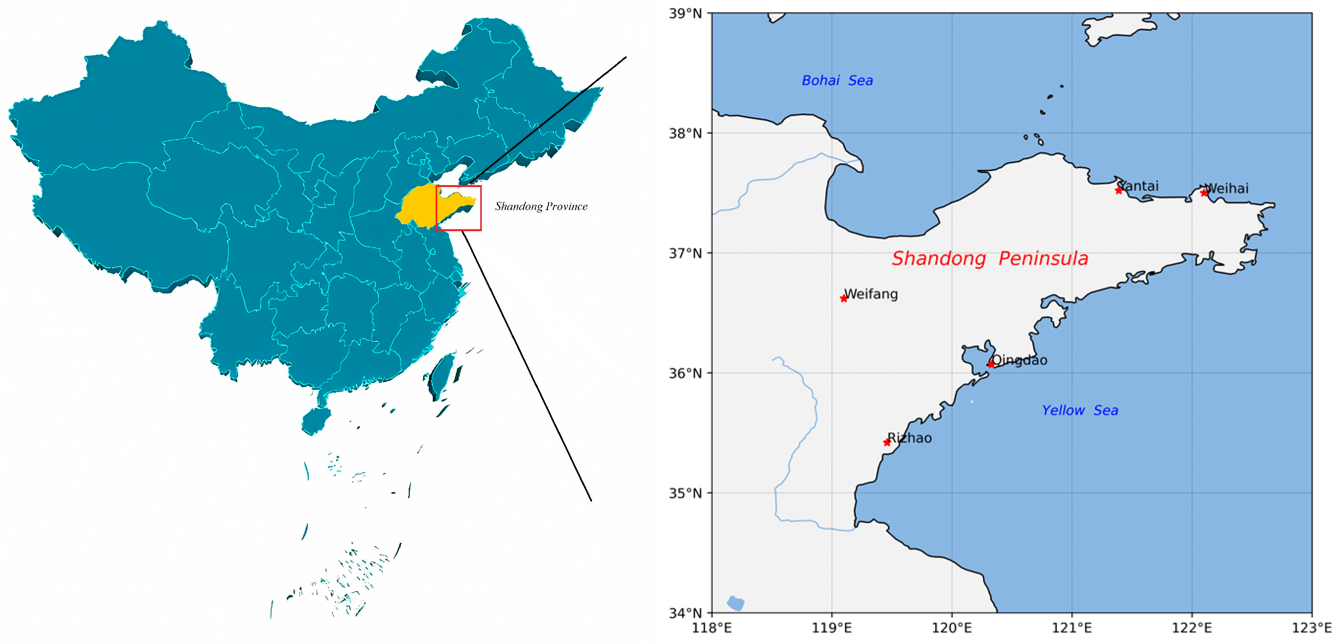
2.1. Study Area

The study focused on 5 coastal cities (Qingdao, Rizhao, Weifang, Weihai and Yantai) on the Shandong Peninsula protruding eastward into the Bohai Sea and the Yellow Sea (Figure 1), which is located in the downwind area of the Northern China Plain, one of the most NO2 polluted regions in China [34,35,36]. Hence, the atmosphere composition on the Shandong Peninsula is the combination of both anthropogenic pollutants from the continent and natural pollutants from the marine atmosphere, which is distinguished from inland cities. High relative humidity caused by frequently occurring sea fog events is the favorable condition for aqueous phase reactions, leading to the production of secondary nitrate aerosols. Sea salt provides the probability of heterogeneous reactions of acid gases such as HNO3, N2O5, and NO2 [37].
The northern half of the peninsula is subject to winter snow and rainstorms and to extensive coastal ice in Weihai and Yantai; the southern half is somewhat warmer in winter. There is less temperature difference during the hot summer months, but the ports (Qingdao, Rizhao, Weihai, and Yantai) are cooler than the interior coastal city (Weifang). Sea fog is common along the north and south coasts of the peninsula.

2.2. Observation Data

We collected daily surface NO2 measurements from the China Air Quality Online Monitoring and Analysis Platform (https://www.aqistudy.cn/) for 1 January 2014–19 September 2020 at five environmental monitoring stations (Figure 1). Meanwhile, we obtained six other regular air pollutants, i.e., CO, O3, SO2, PM10, PM2.5, and Air Quality Index (AQI), where O3 is the 8-h average concentration. Meteorological parameters, including air temperature (AT), air pressure (AirP), relative humidity (RH), wind speed (WS), and wind direction (WD) were from China Meteorological Data Service Center (CMDC) (https://data.cma.cn/ (1 May 2021)) at five environmental monitoring stations. Thus, a total of 13 variables, including six regular air pollutants, five meteorological parameters, and sampling time (month and day) are used as candidate input predictors.
The output predictor of the ML model is the daily average concentrations of NO2 at five coastal cities (Figure 2). It can be seen that the seasonal variations of NO2 concentrations were obvious in all five cities. High concentrations of NO2 were found in the heating season (from November to the following March), while low concentrations were found in the non-heating season.
It is interesting that there is a bimodal distribution of NO2 concentrations every winter during the years 2014–2020, and the latter peak value occurred around Spring Festival (Figure 2). After the holiday, NO2 concentration quickly returned to the original level. The transition became more obvious and of longer duration from the end of January to March 2020 (see red dot lines in Figure 2). This was mainly due to the combined effect of Spring Festival and progressive lockdown from COVID-19 in China [38].
Before we develop the proposed model, data preprocessing was performed to maintain the similarity between dependent and explanatory variables. Scaling data can be achieved by either normalization or standardization. Both goals are to transform features so they can be on a similar scale. In this study, we normalized the input data to make the range of [0, 1] for modelling by Equation (1):
x i = x i x min x max x min
where xi is the input data value of any given point; xmin is the overall minimum and xmax is the overall maximum value. After the forecasting using the trained model, values are then returned to the original values using Equation (1).

3. Methodology

In this study, we use the hybrid model comprised of the RF and Seq2Seq (hereafter RF-S2S) to predict daily surface NO2 concentrations in five coastal cities of northern China. The uses of input selection techniques such as RF increase the efficiency of modelling by selecting the significant input variables and interpreting the behavior of the Seq2Seq model. The RF and Seq2Seq models are described in brief in this section.

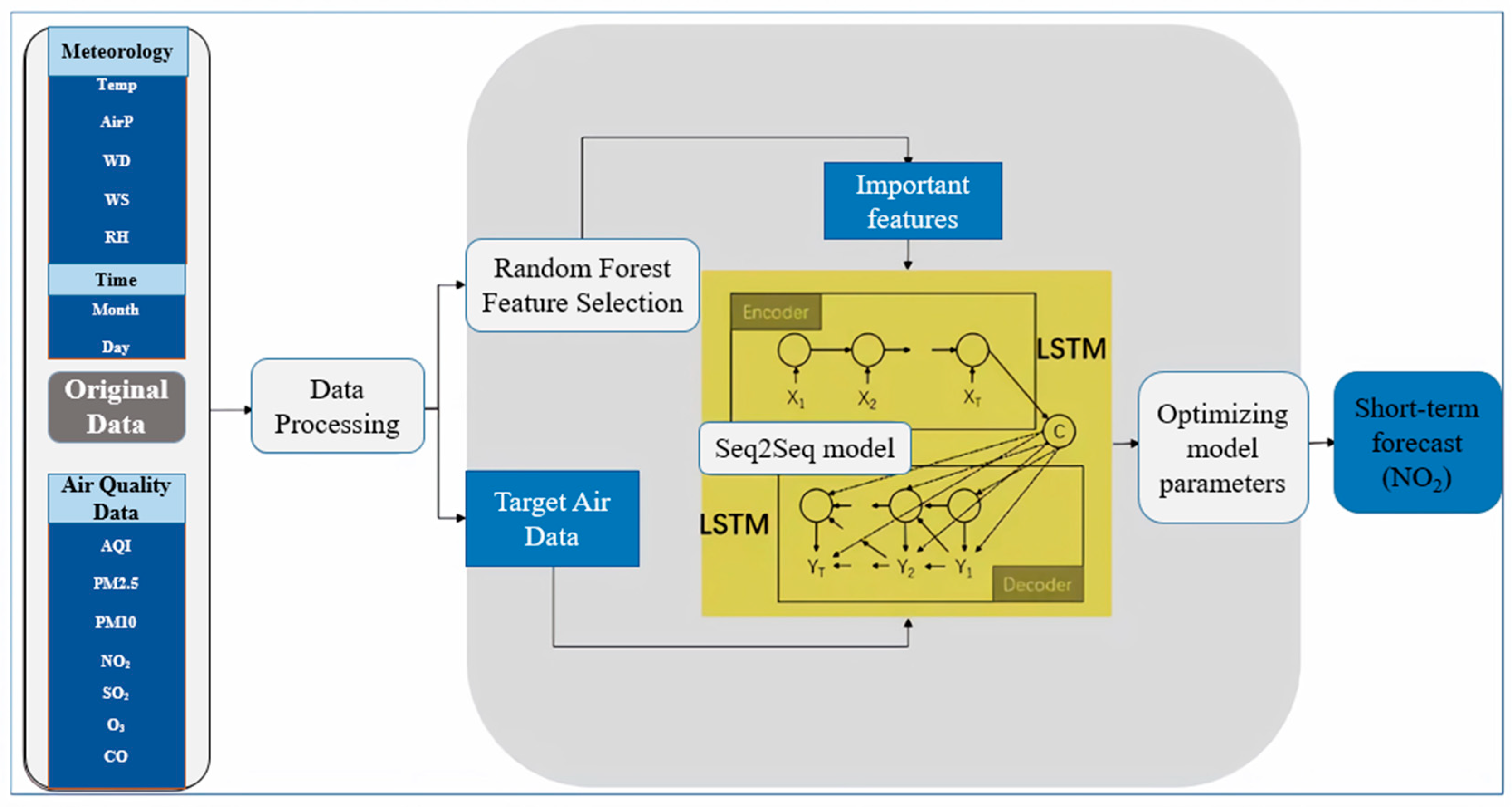
3.1. Hybrid Model Architecture

Figure 3 illustrates the process of 13 candidate variables predicting daily NO2 concentrations by the RF-S2S model. The prediction was performed on the basis of the previous three days to predict the concentration on the next day. After processing original data, they are divided into training and validation data. Training data were used as input to calibrate the model, and validation data validate the model performance. The output sequences (important features in Figure 3) from the feature selection are encoded into the LSTM, and then another LSTM to decode the target sequence (NO2) from the vector. The difference between the generated vector and actual vector forms the loss function, which is used as the mean square error (MSE, Equation (2)) in this study.
M S E = 1 n i = 1 n ( y i y ^ i ) 2
where y i is the value of observed data and y ^ i is the predicted data. By using the back-propagation strategy and optimization algorithm through each training epoch, the model aims to find the minimum value for the loss function.

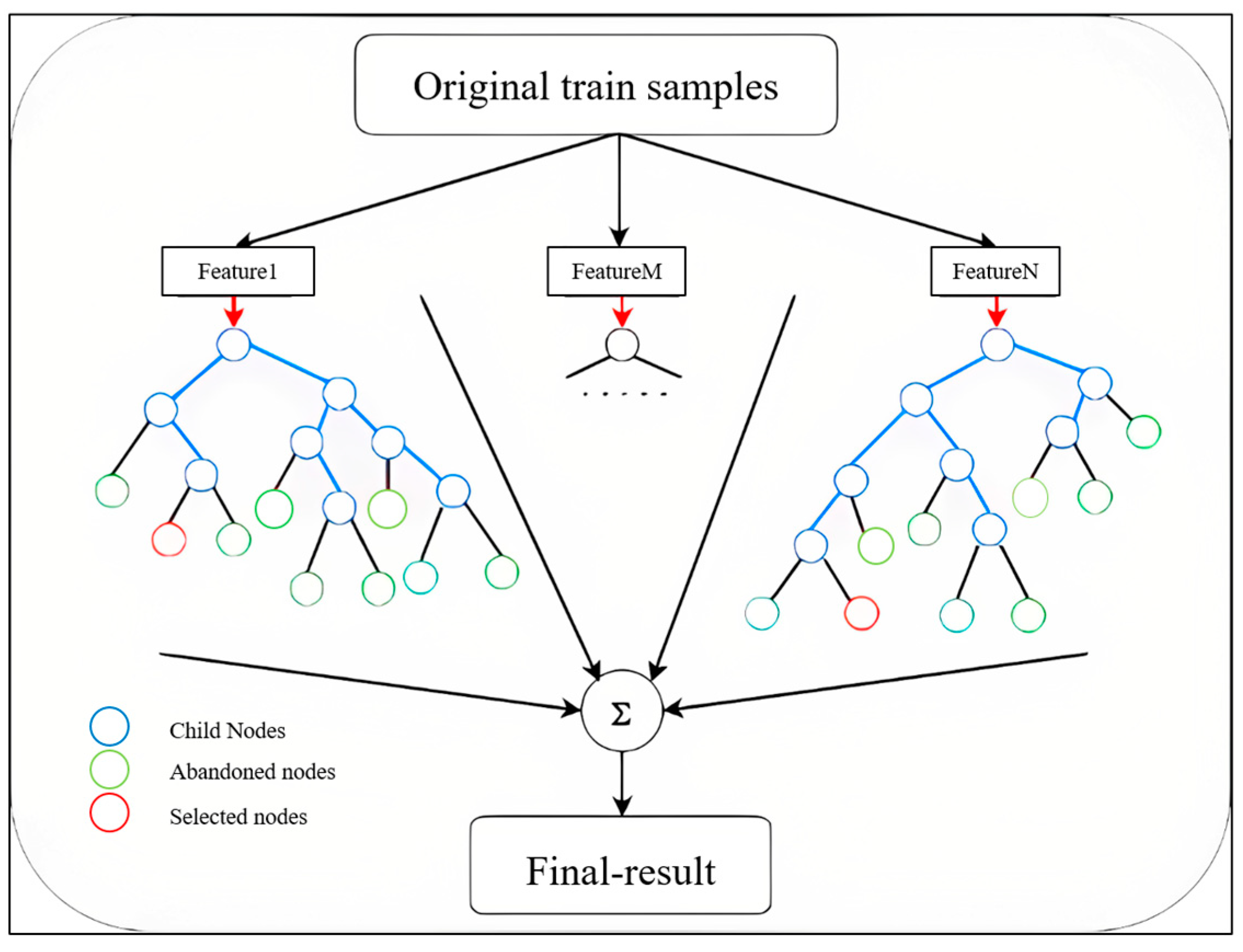
3.2. Feature Selection by Random Forest

Considering the nonlinear relationships among NO2 concentrations, other air pollutants, and meteorological factors, the traditional methods for obtaining the relationship between the input predictors and the output predictor, such as correlation coefficients, support vector machines, and linear regressions are unsatisfactory for handling this complexity. The RF method has been demonstrated to have excellent performance in comparison to traditional logistic regression and linear models [39,40].
The RF methodology was developed as an extension of bagging classification trees in order to reduce variance among single trees, and thus improve prediction accuracy [41]. The Gini criterion is used to select the split with the lowest impurity at each node. For each tree in the forest, the predicted class for each observation is obtained. The class with the maximum number of votes among the trees in the forest is the predicted class of an observation (Figure 4). The estimates of feature importance value (FIV) by the RF model are used to select the best combination of predictor variables. In this study, by adding the FIVs in descending order, the predictors with the sum of FIVs greater than 0.8 remained as the input variables for the surface NO2 prediction by the Seq2Seq model.
RF has also become popular due to its interpretability of the predictor variables, by calculating the FIV for each candidate predictor. Owing to the complex “black box” architecture of the ML models, interpreting the output of these models, compared to simple traditional models, is a demanding task, a major drawback of complex ML algorithms [39,42]. This limitation calls for the development of novel approaches to interpreting the output of ML algorithms.
To ensure the variable features be fairly compared, first, we verify that the estimates of FIV are not influenced by the input order in which the model captures each feature. We take 13 experiments in a random order of 13 candidate predictors (Figure S1). The FIVs in 13 experiments for each predictor clustered around the mean FIV, indicating the availability of RF for selecting features. We applied the classical 0.05 significance threshold to select important features for NO2 prediction [40], interpreting the relationships between the input and output predictors.

3.3. Seq2Seq Prediction Model

The Seq2Seq model is a general end-to-end approach to sequence learning that makes minimal assumptions on the sequence structure, which is well established and used in natural language processing [33]. Figure 3 intermediate module shows the schematic structure of the Seq2Seq model used in this study. Our model includes an encoder and a decoder, each with one LSTM layer inside. Ashtab & Ryoo [27] showed that one- and two-layer LSTM predicted similar results, indicating independence from depths in the performance of the Seq2Seq model. The encoder layer with LSTM cells initially transforms the sequence of inputs into a single vector; then the decoder part transforms the encoder vector into a sequence of outputs. The encoder-decoder architecture is implemented to improve the flexibility of the NO2 forecasting problem.
The Seq2Seq model design variables and hyper-parameters are set manually with a pre-determined value before the training phase (Table 1). These can be considered to be “knobs” which can be turned to tune the deep learning models. These values can be found by a trial-and-error approach, doing the 100% manual search or by grid-search as in this study. For example, the input time steps are set as the past three days after comparison with results of the past one day and seven days (see parameters in the output shape, Table 1). The training set contains the first 85% of the total datasets (including five air pollutants, AQI, historical NO2, 5 meteorological parameters and the sampling time) from 1 January 2014 to 19 September 2019. The remaining 15% of datasets from 20 September 2019 to 19 September 2020 were used for testing. The data on the test set were normalized in a similar manner to those in the training set, with the network output being inversely normalized to the original unit. The random seed is used to reproduce the same output data multiple times.
In addition to the RF-S2S model, we also test the ability of four other models, including the Seq2Seq model without RF feature selection and the LSTM model with and without feature selection. To make an apple-to-apple comparison, we train and test all of the models used in this study on the same samples.

3.4. Model Evaluation

Several statistical metrics are used in this study to evaluate the performance of the stacked RF-S2S and other four models. The commonly used model score metrics, such as the Nash–Sutcliffe coefficient (NS), Pearson’s correlation coefficient (Pearson’s r), the Root Mean Square Error (RMSE), the Mean Absolute Error (MAE) and the Mean Absolute Percentage Error (MAPE) (Equations (3)–(7)) were used. The NS is normalised metric that is widely used for evaluating forecasted results [43]. It ranges from −∞ to 1, an efficiency of 1 corresponds to a perfect match of predicted data to the observed data. The values of Pearson’s r between 0.7 and 1.0 (−0.7 and −1.0) indicate a strong approximate (symmetric) shape of the individual predicted data and observed data. RMSE is the measure for determining the better model. The smaller the RMSE value, the better the model, viz., the more precise the predictions. MAE and MAPE are used to evaluate the proximity between the predicted results and the observations.
N S = i = 1 n ( y ^ i y ¯ ) 2 i = 1 n ( y i y ¯ ) 2 ,
P e a r s o n s   r = i = 1 n ( y ^ i y ^ ¯ i ) ( y i y ¯ i ) i = 1 n ( y i y ^ ¯ i ) 2 i = 1 n ( y ^ i y ¯ i ) 2 ,
R M S E = 1 n i = 1 n ( y ^ i y i ) 2 ,
M A E = 1 n i = 1 n | y ^ i y i | ,
M A P E = 100 % n i = 1 n | y ^ i y i y i | ,
where y i is the value of observed data, y ^ i is the predicted data, y ¯ i and y ^ ¯ i are mean values of observed data and predicted data, respectively.

4. Results and Discussion

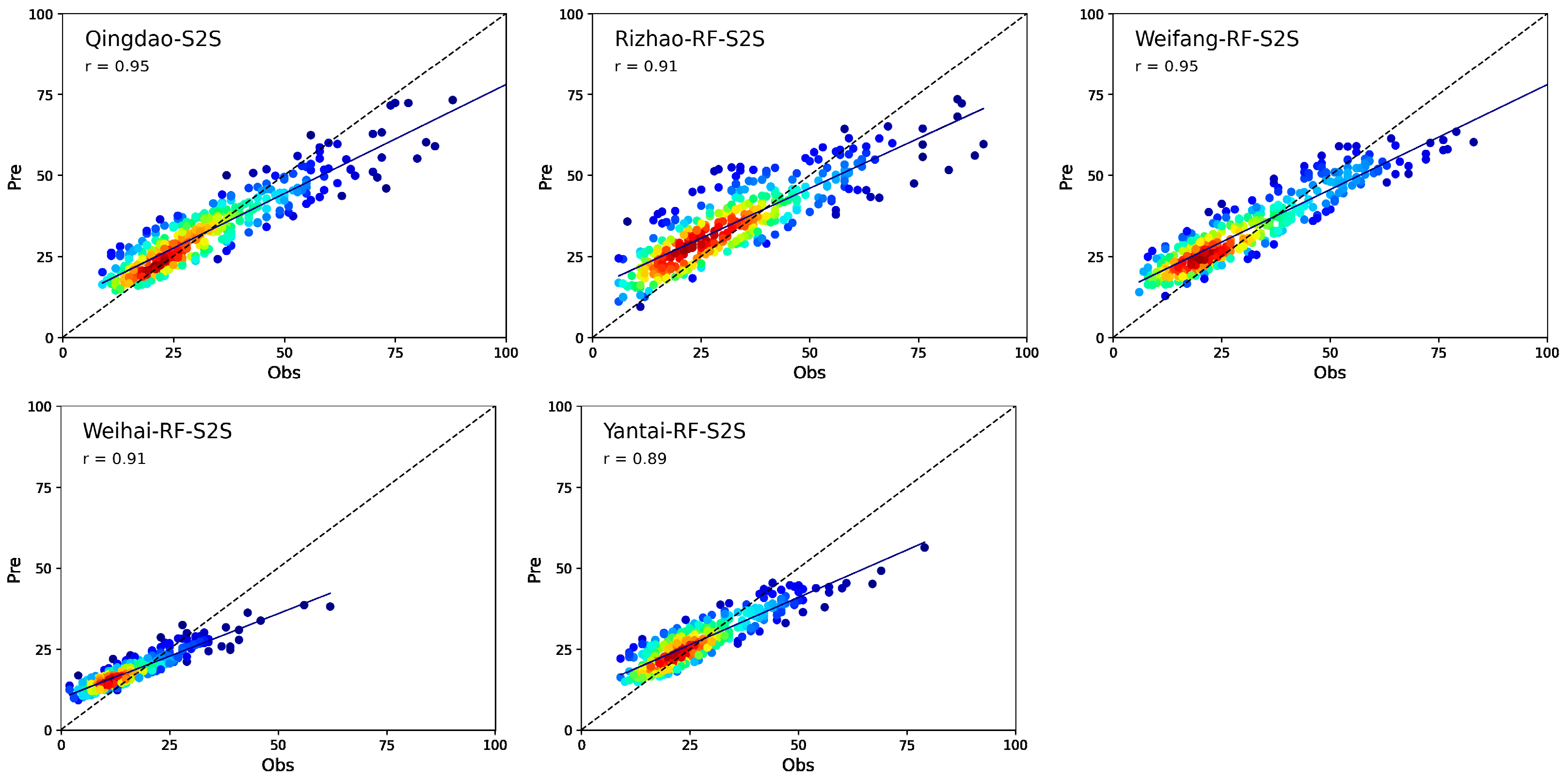
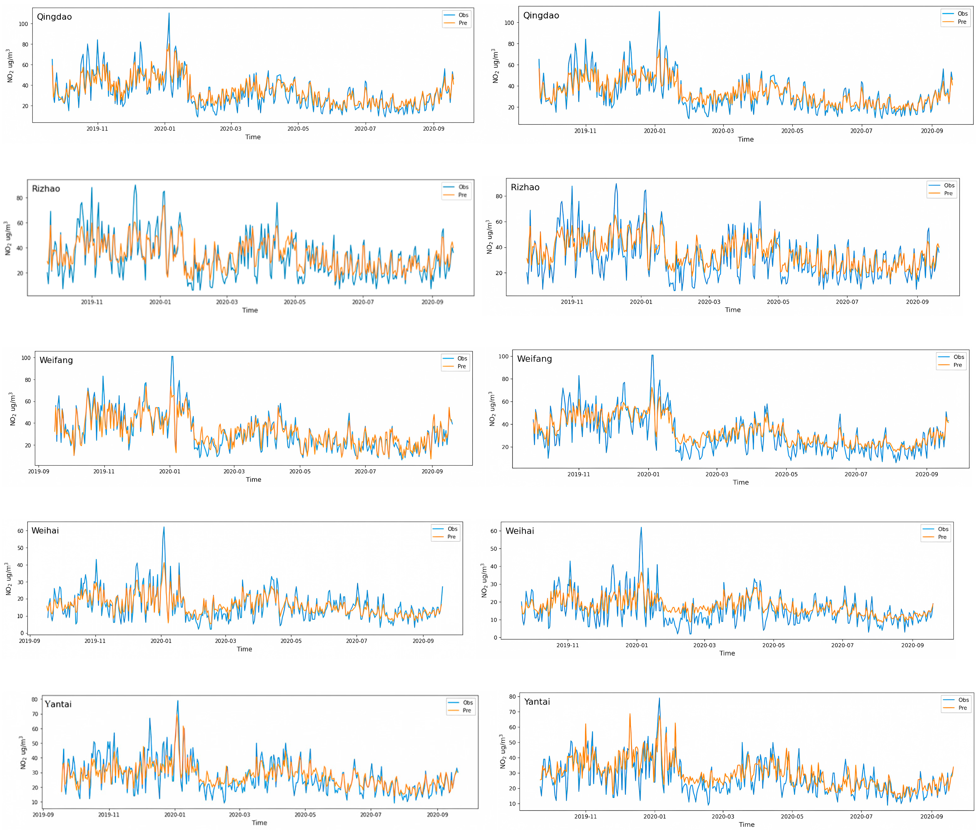
4.1. Evaluation of RF-S2S Model

Table 2 summarizes the RF selection features in five coastal cities of northern China, with the sum of FIVs larger than 0.8. CO and PM10 are two common features as the input variables in all five coastal cities. RH and AirP are selected as input predictors in four coastal cities.
After evaluating the model performance on a training set, we applied the RF-S2S model to a test set. The density scatter plots of the predicted vs. observed NO2 concentrations in 5 coastal cities are illustrated Figure 5. The modelled NO2 concentrations from the test set are closely comparable with the observed values in each city. Most of the data are close to the bisector (the black dashed lines in Figure 5), especially under low NO2 pollution conditions. The slopes of the fitted linear were less than one, which is mainly caused by heavy pollution episodes. The high correlation coefficient (mean Pearson’s r = 0.93) suggests that the goodness of RF-S2S model performance, with a slight underestimation of the observed NO2 in Rizhao. This result suggests that, despite some episodic signals, the network model has a good robustness and can accurately forecast NO2 concentrations one day in advance.
Table 3 represents the accuracy of the RF-S2S model at predicting NO2 concentrations. The average value of NS in five cities is 0.79, suggesting that the selected features as input variables in each city can approximately explain 80% of daily NO2 variability. The MAPEs from 16% to 26% in in five cities reveal a small divergence between the predicted values and observed values. The low average RMSE of 5.85 µg/m3, along with a low mean MAE of 4.5 µg/m3, indicate that the RF-S2S model produces highly accurate estimates of daily NO2 concentrations.

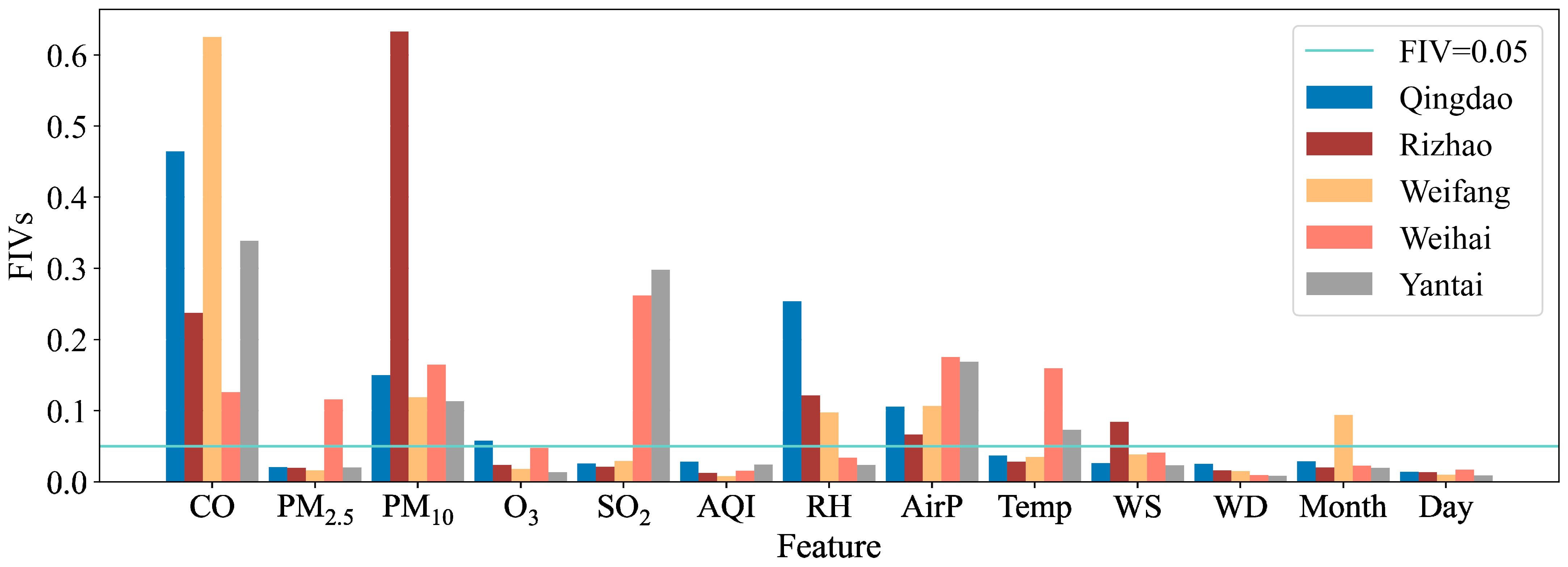
4.2. Important Features Influencing NO2 Prediction

The main aim of feature selection has two parts: one is to find the most efficient set of input variables that can perform equally to the whole group of variables or even outperform it; the other is to interpret the Seq2Seq model for predicting NO2 concentration. Figure 6 presents the FIVs of all 13 factors contributing to forecasting NO2 output fluctuations. Compared to meteorological factors, gaseous pollutants have an important influence on NO2 prediction with the largest FIV about 0.5 in most of the coastal cities, implying a common source of air pollution mainly from anthropogenic factors. Previous research showed that coal consumption and transportation were superior factors affecting the atmospheric NO2 concentration in the coastal cities of the Shandong peninsula in China [44,45]. In Weihai city, the large FIV is less than 0.2, and the notable features include air pressure and air temperature. This result indicates that air pollution in Weihai is controlled by both anthropogenic sources and meteorological conditions, which has also been found numerically by Xing et al. [46] using a numerical model.
CO is selected as the commonly important feature in four coastal cities. Especially in Qingdao, Weifang, and Yantai, the relation between NO2 and CO is the closest compared with other four gaseous pollutants (PM10, PM2.5, SO2, and O3). Similar results have been found in another coastal city of China [29]. Wang et al. [47] also found significant Pearson’s correlations between NO2 and CO in 31 provincial capital cities of China between 2013 and 2014. It is reasonable to consider this to be due to the transportation sector being closely related to the emission of NO2 and CO in most cities of China [47,48]. PM10 is another commonly important feature in five coastal cities. It is the most important feature influencing NO2 prediction in Rizhao, with FIV over 0.6. In the northern coastal cities of Shandong peninsula, Yantai, and Weihai, SO2 is selected as an important feature with FIVs ranging between 0.14~0.15. However, on the southern coast of the peninsula, the FIV of SO2 is about 0.03, below the selection standard value 0.05.
Among with the meteorological factors, air pressure has an important influence on NO2 prediction. Following that is RH, especially for the southern coast, implying the effect of marine climate on NO2 concentration. Wind (speed and direction) has a minor effect on the NO2 prediction in coastal cities.

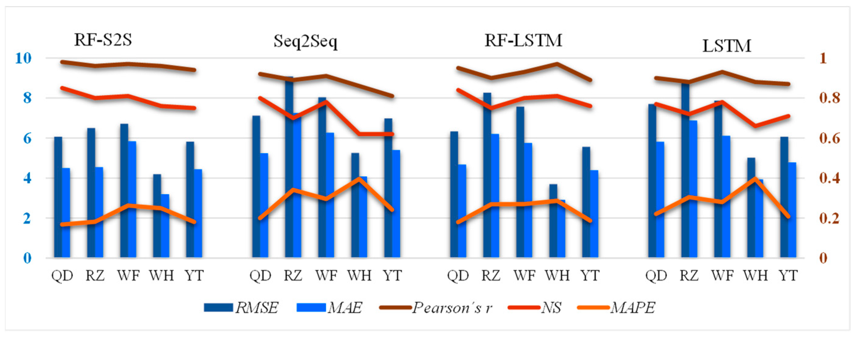
4.3. Comparison with Other Deep Sequence Learning Models without Feature Selection

The Seq2Seq model was trained with the whole data variations as alternative input in each city. Figure 7 represents the comparison of each alternative for Seq2Seq models with and without feature selection. Through visual analysis, it can be seen that the prediction curve of the Seq2Seq model without feature selection is relatively flat (Figure 7, right panel), making it difficult to accurately predict the fluctuation of data, especially from February to August with lower NO2 concentrations. The RF-S2S model performs better on the fluctuation and the outliers (maxima and minima) of the data, especially in Weifang, Yantai, and Rizhao. Although Spring Festival and the outbreak of the COVID-19 pandemic made the NO2 concentrations decrease more extreme and the transition last longer in 2020 than in the previous year [38], the RF-S2S model still predicted this feature fairly well (Figure 7, left panel), with some overestimation on the northern coastal of Shandong peninsula (Weihai and Yantai). In general, we indicate that the feature selection should be helpful to improve the prediction efficiency and accuracy of Seq2Seq models by screening and selecting the significant inputs.
The values of statistical indices can explain the above phenomena (Figure 8). The average value of NSs in five coastal cities obtained by the RF-S2S model increases by 13%, compared to the Seq2Seq model without feature selection (from 0.70 to 0.79). Similarly, performing feature selection leads to an increase of Pearson’s r in each city, with an average value from 0.88 to 0.96. However, errors (RMSE, MAE, and MAPE) decline significantly by extracting features before implementing the Seq2Seq model, about 19.7%, 20.3%, and 29.3%, respectively. Thus, the RF-feature selection proved effective in improving the performance of deep learning models. The RF algorithms, one of the important wrapper methods, has been widely recognized as a practical method of variable selection [49,50]. For example, Shamsoddini et al. [50] indicated that the feasibility of the RF method for improving the MLP performance in prediction of the air pollutants in Tehran. Ashtab & Ryoo [27] found that among the Seq2Seq models using different feature selection algorithms, RF-feature selection results as their inputs performed better than other wrappers as well as filter methods. Furthermore, the demand for variable selection has been increasing [31].
In addition, we compared the performance of the RF-S2S model with RF-LSTM and the single LSTM model (Figure 8). Compared to the RF-S2S model results, the mean values of NS and Pearson’s r obtained by the LSTM models with and without feature selection decrease, while RMSE, MAE and MAPE increase significantly. All four models predicted much more accurately on the southern coast of the peninsula than in the northern part, with a higher mean value of NS and Pearson’s r and a lower mean value of MAPE in Qingdao, Rizhao, and Weifang (0.93, 0.78, 0.25, respectively) than that in Weihai and Yantai (0.89, 0.71, 0.27, respectively). The LSTM model with RF-feature selection performed better than the standalone models (Seq2Seq, LSTM), especially in the northern coastal areas. In general, the RF-S2S model outperformed the LSTM models with and without feature selection, and the RF-LSTM model has a similar capability to the RF-S2S model in the northern coast of the peninsula.
The Seq2Seq model based on LSTM units is a special architecture that maps a sequence of input data (encoder) to another sequence of output data (decoder). This arrangement effectively removes the restriction for a standalone LSTM that the length of input sequence should be uniform with each other. Because the encoder LSTM can unroll the input sequence along the temporal axis as many times as it lasts, while the decoder LSTM always unrolls a predefined number of times to be compatible with the other layers on the top of it [51]. Thus, the Seq2Seq model exhibited superiority in dealing with variable-length input and output sequences time series data prediction than a simple LSTM [27]. However, reasons for comparable performances between Seq2Seq and LSTM in the northern part of Shandong peninsula remained to be determined.

4.4. Limitation and Improvement Project

Despite the satisfactory performance of our RF-S2S models in forecasting NO2 concentrations in five coastal cities of northern China, they cannot predict high concentrations well on heavy pollution days. For example, in Qingdao city, the prediction of the RF-S2S model is less than observation over 25 µg/m3 on the two maxima of day 42 (1 November 2019) and day 107 (5 January 2020) (Figure 7, top left panel). This is mainly due to the shortage of historical data of heavy pollution days, making training data limited and hence leading to great uncertainty in the prediction of high values [29].
In addition, significant variation of NO2 concentrations from 2014 to 2020 is an important obstacle to improving prediction accuracy, especially in northern coast of Shandong peninsula. The execution the Clean Air Action Plan (CAAP; 2013–2017) and the Blue Sky Protection Campaign (BSPC; 2018–2020) enacted in China reduced NO2 pollution in coastal areas [36,52]. For example, Liu et al. [52] found that the annual mean levels of NO2 declined by 8% from 2015 to 2020 in Qingdao. Meng et al. [53] showed that the seasonal mean concentrations of NO2 generally decreased from 2013 to 2017 but increased unexpectedly in 2018 in Qingdao.
We explore temporal variations by the EMD method (detailed introduction in Supplementary). Figure S2 shows the temporal time-series signal of intrinsic mode functions (IMFs) and residuals (RES) from the EMD transformation of NO2 in five coastal cities. The IMF7 with a time scale of ~7 months (Equation (S2)) indicates that the seasonal periodic change rule remained unchanged in Qingdao and Rizhao during 2014–2019, while the peak values in the heating season showed a downward trend in 2020 due to the outbreak of COVID-19. The time scale of IMF8 is about 16 months, which approximately reflects the interannual variation of NO2. Contrary to the seasonality, the interannual variation of NO2 in the southeast coast of Shandong peninsula is smaller than that in the northern part, which takes on an evident process in different years. From the RES, we found that during 2014–2018, NO2 concentrations were basically flat, while they declined since 2019 on the southern coast of the Shandong peninsula (Qingdao and Rizhao). On the northern coast, NO2 concentrations declined steadily during 2014–2020.
In general, a more significant decreasing trend occurred on the northern coast of the Shandong peninsula than in the southern regions. Dramatic changes regulated by emission control policies are likely the reason for weaker predicting accuracy on the northern coast of the Shandong peninsula, which is not well caught by the RF-S2S model. Therefore, performing data decomposition and extracting variations at different time scales before implementing deep learning models is proposed to improve the prediction accuracy [28,29]. To further overcome computational load on data decomposition-based deep learning models, a hybrid deep learning model combined with feature selection and data decomposition will provide useful insights on how NO2 parameters can help to efficiently perform short-term forecasting.
Moreover, as a data-driven model, the RF-S2S mainly relies on the empirical formula of meteorological parameters and historical monitoring data, failing to consider the atmospheric chemical transformation, pollution source emission change, and regional transmission process. Shipping emissions [54] and sea breezes [44] are especially important parameters influencing NO2 concentrations in coastal areas.

5. Conclusions

In this study, a hybrid model (RF-S2S) was established based on RF feature selection and a Seq2Seq method to predict NO2 concentration in coastal cities of northern China. The research findings are as follows:
The data set is fed into RF algorithms to filter out the most significant features influencing NO2 concentration, which are also used to describe how the Seq2Seq model understands the predictor variable. The influence of gaseous pollutants on NO2 prediction is more important than that of meteorological factors. CO and PM10 are two common, important features in five coastal cities of northern China.
The output sequences from the RF feature selection were fed into the Seq2Seq model to determine the best features. The RF feature selection proved effective in enhancing the performance of Seq2Seq models, by reducing errors (RMSE, MAE, and MAPE) over 20%. Our RF-S2S models outperformed traditional LSTM models with and without feature selection, which can capture general trends and disruptions of NO2 concentrations due to air quality control policies, winter heating, and the Spring Festival holiday.
Considering significant variations of NO2 concentrations on different time scales in coastal areas of northern China, performing data decomposition before training the RF-S2S hybrid model is our next step to improve the prediction accuracy of NO2 concentration.

Supplementary Materials

The following supporting information can be downloaded at: https://www.mdpi.com/article/10.3390/atmos14030467/s1, Figure S1. Boxplots of random forest experiments with in a random order of 13 candidate predictors; Text S1. Introduction of EMD method; Figure S2. Temporal time-series signal of intrinsic mode functions (IMFs) and residuals (RES) from the EMD transformation of NO2 concentration at 5 coastal cities of the northern China.

Author Contributions

Conceptualization, X.G. and H.G.; Data curation, X.J.; Formal analysis, G.L. and X.L.; Funding acquisition, H.G.; Investigation, X.J., X.G., X.Z., H.M. and X.L.; Methodology, X.J. and X.G.; Project administration, X.G.; Resources, X.G.; Software, X.J.; Supervision, H.G.; Validation, X.J.; Visualization, X.J.; Writing—original draft, X.G. and X.J.; Writing—review and editing, X.G., Q.D. and X.L. All authors have read and agreed to the published version of the manuscript.

Funding

This work was supported by the National Nature Science Foundation of China-Shandong Joint Fund (U1906215), the National Natural Science Foundation of China (42175129) and Qingdao University of Science and Technology Postgraduate Independent Research Innovation Special (S2022KY029).

Institutional Review Board Statement

Not applicable.

Informed Consent Statement

Not applicable.

Data Availability Statement

Restrictions apply to the availability of these data. Not all data are available as some of the data relate to further research and can be obtained by contacting the authors.

Acknowledgments

We would like to acknowledge Xiaohong Yao, Xinyu Guo and Jianqiang Chen for valuable advice and programming assistance.

Conflicts of Interest

The authors declare no conflict of interest.

References

  1. Zhu, F.; Ding, R.; Lei, R.; Cheng, H.; Liu, J.; Shen, C.; Cao, J. The short-term effects of air pollution on respiratory diseases and lung cancer mortality in Hefei: A time-series analysis. Respir. Med. 2019, 146, 57–65. [Google Scholar] [CrossRef]
  2. Zheng, J.; Jiang, P.; Qiao, W.; Zhu, Y.; Kennedy, E. Analysis of air pollution reduction and climate change mitigation in the industry sector of Yangtze River Delta in China. J. Clean. Prod. 2016, 114, 314–322. [Google Scholar] [CrossRef]
  3. Long, L.B.; She, Q.N.; Meng, Z.Q.; Liu, M.; Zhu, Y.; Yan, Y.Y. Characteristics and cluster analysis of air pollution in coastal areas of China. Res. Environ. Sci. 2018, 31, 2063–2072. [Google Scholar] [CrossRef]
  4. Zheng, Y.; Liu, F.; Hsieh, H.P. U-air: When urban air quality inference meets big data. In Proceedings of the 19th ACM SIGKDD International Conference on Knowledge Discovery and Data Mining, Chicago, IL, USA, 11–14 August 2013; pp. 1436–1444. [Google Scholar] [CrossRef]
  5. Cao, Q.; Shen, L.; Chen, S.C.; Pui, D.Y.H. WRF modeling of PM2.5 remediation by SALSCS and its clean air flow over Beijing terrain. Sci. Total Environ. 2018, 626, 134–146. [Google Scholar] [CrossRef]
  6. Zhang, Q.; Xue, D.; Liu, X.H.; Gong, X.; Gao, H.W. Process analysis of PM2.5 pollution events in a coastal city of China using CMAQ. J. Environ. Sci. 2019, 79, 225–238. [Google Scholar] [CrossRef]
  7. Yu, S.; Zhang, Q.; Yan, R.; Wang, S.; Li, P.; Chen, B.; Liu, W.; Zhang, X. Origin of air pollution during a weekly heavy haze episode in Hangzhou, China. Environ. Chem. Lett. 2014, 12, 543–550. [Google Scholar] [CrossRef]
  8. Wang, D.; Jiang, B.; Li, F.; Lin, W. Investigation of the air pollution event in Beijing-Tianjin-Hebei region in December 2016 using WRF-chem. Adv. Meteorol. 2018, 2018, 1634578. [Google Scholar] [CrossRef]
  9. Rahimi, A. Short-term prediction of NO2 and NOx concentrations using multilayer perceptron neural network: A case study of Tabriz, Iran. Ecol. Process. 2017, 6, 4. [Google Scholar] [CrossRef] [Green Version]
  10. Navares, R.; Aznarte, J.L. Predicting air quality with deep learning LSTM: Towards comprehensive models. Ecol. Inform. 2020, 55, 101019. [Google Scholar] [CrossRef]
  11. Sayeed, A.; Choi, Y.; Eslami, E.; Lops, Y.; Roy, A.; Jung, J. Using a deep convolutional neural network to predict 2017 ozone concentrations, 24 hours in advance. Neural Netw. 2020, 121, 396–408. [Google Scholar] [CrossRef]
  12. Mehmood, K.; Bao, Y.; Cheng, W.; Khan, M.A.; Siddique, N.; Abrar, M.M.; Naidu, R. Predicting the quality of air with machine learning approaches: Current research priorities and future perspectives. J. Clean. Prod. 2022, 379, 134656. [Google Scholar] [CrossRef]
  13. Brunelli, U.; Piazza, V.; Pignato, L.; Sorbello, F.; Vitabile, S. Two-days ahead prediction of daily maximum concentrations of SO2, O3, PM10, NO2, CO in the urban area of Palermo, Italy. Atmos. Environ. 2007, 41, 2967–2995. [Google Scholar] [CrossRef]
  14. Li, X.; Peng, L.; Yao, X.; Cui, S.; Hu, Y.; You, C.; Chi, T. Long short-term memory neural network for air pollutant concentration predictions: Method development and evaluation. Environ. Pollut. 2017, 231, 997–1004. [Google Scholar] [CrossRef] [PubMed]
  15. Reddy, V.; Yedavalli, P.; Mohanty, S.; Nakhat, U. Deep air: Forecasting air pollution in Beijing, China. In Proceedings of the 2017 IEEE International Conference on Computer Vision (ICCV), Venice, Italy, 22–29 October 2017; pp. 1–9. [Google Scholar]
  16. Qi, Y.; Li, Q.; Karimian, H.; Liu, D. A hybrid model for spatiotemporal forecasting of PM2.5 based on graph convolutional neural network and long short-term memory. Sci. Total Environ. 2019, 664, 1–10. [Google Scholar] [CrossRef]
  17. Iskandaryan, D.; Ramos, F.; Trilles, S. Graph Neural Network for Air Quality Prediction: A Case Study in Madrid. IEEE Access 2023, 11, 2729–2742. [Google Scholar] [CrossRef]
  18. Yu, X.; Shi, S.; Xu, L. A spatial–temporal graph attention network approach for air temperature forecasting. Appl. Soft Comput. 2021, 113, 107888. [Google Scholar] [CrossRef]
  19. Jiang, W.; Luo, J. Graph neural network for traffic forecasting: A survey. Expert Syst. Appl. 2022, 207, 117921. [Google Scholar] [CrossRef]
  20. Bui, K.H.N.; Cho, J.; Yi, H. Spatial-temporal graph neural network for traffic forecasting: An overview and open research issues. Appl. Intell. 2022, 52, 2763–2774. [Google Scholar] [CrossRef]
  21. Ouyang, X.; Yang, Y.; Zhang, Y.; Zhou, W. Spatial-temporal dynamic graph convolution neural network for air quality prediction. In Proceedings of the 2021 International Joint Conference on Neural Networks (IJCNN), Shenzhen, China, 18–22 July 2021; pp. 1–8. [Google Scholar] [CrossRef]
  22. Ge, L.; Wu, K.; Zeng, Y.; Chang, F.; Wang, Y.; Li, S. Multi-scale spatiotemporal graph convolution network for air quality prediction. Appl. Intell. 2021, 51, 3491–3505. [Google Scholar] [CrossRef]
  23. Wang, C.; Zhu, Y.; Zang, T.; Liu, H.; Yu, J. Modeling inter-station relationships with attentive temporal graph convolutional network for air quality prediction. In Proceedings of the 14th ACM International Conference on Web Search and Data Mining, Jerusalem, Israel, 8–12 March 2021; pp. 616–634. [Google Scholar] [CrossRef]
  24. Cabaneros, S.M.S.; Calautit, J.K.S.; Hughes, B.R. Hybrid artificial neural network models for effective prediction and mitigation of urban roadside NO2 pollution. Energy Procedia 2017, 142, 3524–3530. [Google Scholar] [CrossRef]
  25. Ma, J.; Ding, Y.; Cheng, J.C.; Jiang, F.; Wan, Z. A temporal-spatial interpolation and extrapolation method based on geographic Long Short-Term Memory neural network for PM2.5. J. Clean. Prod. 2019, 237, 117729. [Google Scholar] [CrossRef]
  26. Zhou, S.; Bethel, B.J.; Sun, W.; Zhao, Y.; Xie, W.; Dong, C. Improving Significant Wave Height Forecasts Using a Joint Empirical Mode Decomposition–Long Short-Term Memory Network. J. Mar. Sci. Eng. 2021, 9, 744. [Google Scholar] [CrossRef]
  27. Ashtab, M.; Ryoo, B.Y. Predicting Construction Workforce Demand Using a Combination of Feature Selection and Multivariate Deep-Learning Seq2seq Models. J. Constr. Eng. Manag. 2022, 148, 04022136. [Google Scholar] [CrossRef]
  28. Bai, Y.; Zeng, B.; Li, C.; Zhang, J. An ensemble long short-term memory neural network for hourly PM2.5 concentration forecasting. Chemosphere 2019, 222, 286–294. [Google Scholar] [CrossRef] [PubMed]
  29. Liu, B.C.; Zhang, L.; Wang, Q.S.; Chen, J. A Novel Method for Regional NO2 Concentration Prediction Using Discrete Wavelet Transform and an LSTM Network. Comput. Intell. Neurosci. 2021, 2021, 6631614. [Google Scholar] [CrossRef] [PubMed]
  30. Wang, Y.; Wu, L. On practical challenges of decomposition-based hybrid forecasting algorithms for wind speed and solar irradiation. Energy 2016, 112, 208–220. [Google Scholar] [CrossRef] [Green Version]
  31. Qian, Z.; Pei, Y.; Zareipour, H.; Chen, N. A review and discussion of decomposition-based hybrid models for wind energy forecasting applications. Appl. Energy 2019, 235, 939–953. [Google Scholar] [CrossRef]
  32. Chen, R.C.; Dewi, C.; Huang, S.W.; Caraka, R.E. Selecting critical features for data classification based on machine learning methods. J. Big Data 2020, 7, 52. [Google Scholar] [CrossRef]
  33. Sutskever, I.; Vinyals, O.; Le, Q.V. Sequence to Sequence Learning with Neural Networks. In Proceedings of the 27th International Conference on Neural Information Processing Systems, Montreal, QC, Canada, 8–13 December 2014; pp. 3104–3112. [Google Scholar]
  34. Chan, C.K.; Yao, X.H. Air pollution in mega cities in China. Atmos. Environ. 2008, 42, 1–42. [Google Scholar] [CrossRef]
  35. Liu, L.; Bei, N.; Hu, B.; Wu, J.R.; Liu, S.X.; Li, X.; Wang, R.N.; Liu, Z.R.; Shen, Z.X.; Li, G.H. Wintertime nitrate formation pathways in the north China plain: Importance of N2O5 heterogeneous hydrolysis. Environ. Pollut. 2020, 266, 115287. [Google Scholar] [CrossRef]
  36. Zhang, Y.; Zhou, R.; Chen, J.; Rangel-Buitrago, N. The effectiveness of emission control policies in regulating air pollution over coastal ports of China: Spatiotemporal variations of NO2 and SO2. Ocean Coast. Manag. 2022, 219, 106064. [Google Scholar] [CrossRef]
  37. Carvalho, A.R.; Gama, C.; Monteiro, A. Investigating the contribution of sea salt to PM10 concentration values on the coast of Portugal. Air Qual. Atmos. Health 2021, 14, 1697–1708. [Google Scholar] [CrossRef]
  38. Bao, R.; Zhang, A. Does lockdown reduce air pollution? Evidence from 44 cities in northern China. Sci. Total Environ. 2020, 731, 139052. [Google Scholar] [CrossRef] [PubMed]
  39. Archer, K.J.; Kimes, R.V. Empirical characterization of random forest variable importance measures. Comput. Stat. Data Anal. 2008, 52, 2249–2260. [Google Scholar] [CrossRef]
  40. Altmann, A.; Toloşi, L.; Sander, O.; Lengauer, T. Permutation importance: A corrected feature importance measure. Bioinformatics 2010, 26, 1340–1347. [Google Scholar] [CrossRef] [Green Version]
  41. Breiman, L. Random Forests. Mach. Learn. 2001, 45, 5–32. [Google Scholar] [CrossRef] [Green Version]
  42. García, M.V.; Aznarte, J.L. Shapley additive explanations for NO2 forecasting. Ecol. Inform. 2020, 56, 101039. [Google Scholar] [CrossRef]
  43. McCuen, R.H.; Knight, Z.; Cutter, A.G. Evaluation of the Nash-Sutcliffe efficiency index. J. Hydrol. Eng. 2006, 11, 597–602. [Google Scholar] [CrossRef]
  44. Xue, Y.; Peng, Z.; Liu, L. Analysis of distribution characteristics and influencing factors of air pollutants in typical coastal cities. Energy Environ. Prot. 2021, 35, 94–101. [Google Scholar]
  45. Li, M.; Li, S.; Li, D.Z.; Jiang, S.W.; Xu, S. Analysis and Prediction of Qingdao Atmospheric NO2 Concentration Factors. J. Environ. Sci. Manag. 2016, 41, 130–134. [Google Scholar]
  46. Xing, Z.W.; Wei, M.; Ning, W.T.; Zhang, M.G.; Li, K.; Jiang, W. Study on the cause of air pollution rebound in Weihai in early 2019 based on RAMS-CMAQ simulation. Acta Sci. Circumstantiae 2021, 41, 886–897. [Google Scholar] [CrossRef]
  47. Wang, Y.; Ying, Q.; Hu, J.; Zhang, H. Spatial and temporal variations of six criteria air pollutants in 31 provincial capital cities in China during 2013–2014. Environ. Int. 2014, 73, 413–422. [Google Scholar] [CrossRef] [PubMed]
  48. Zou, C.; Wu, L.; Li, X.Y.; Yuan, Y.; Jing, B.; Mao, H.J. Relationship between traffic flow and temporal and spatial variations of NO2 and CO in Nanjing. Acta Sci. Circumstantiae 2017, 37, 3894–3905. [Google Scholar] [CrossRef]
  49. Salcedo-Sanz, S.; Cornejo-Bueno, L.; Prieto, L.; Paredes, D.; García-Herrera, R. Feature selection in machine learning prediction systems for renewable energy applications. Renew. Sustain. Energy Rev. 2018, 90, 728–741. [Google Scholar] [CrossRef]
  50. Shamsoddini, A.; Aboodi, M.R.; Karami, J. Tehran air pollutants prediction based on random forest feature selection method. Int. Arch. Photogramm. Remote Sens. Spat. Inf. Sci. 2017, 42, 4. [Google Scholar] [CrossRef] [Green Version]
  51. Tang, Y.; Xu, J.; Matsumoto, K.; Ono, C. Sequence-to-Sequence Model with Attention for Time Series Classification. In Proceedings of the 2016 IEEE 16th International Conference on Data Mining Workshops (ICDMW), Barcelona, Spain, 12–15 December 2016; pp. 503–510. [Google Scholar] [CrossRef]
  52. Liu, B.; Wang, Y.; Meng, H.; Dai, Q.; Diao, L.; Wu, J.; Feng, Y. Dramatic changes in atmospheric pollution source contributions for a coastal megacity in northern China from 2011 to 2020. Atmos. Chem. Phys. 2022, 22, 8597–8615. [Google Scholar] [CrossRef]
  53. Meng, H.; Shen, Y.; Fang, Y.; Zhu, Y. Impact of the ‘Coal-to-Natural Gas’ Policy on Criteria Air Pollutants in Northern China. Atmosphere 2022, 13, 945. [Google Scholar] [CrossRef]
  54. Tan, W.; Liu, C.; Wang, S.S.; Xing, C.Z.; Su, W.J.; Zhang, C.X.; Xia, C.Z.; Liu, H.R.; Cai, Z.N.; Liu, J.G. Tropospheric NO2, SO2, and HCHO over the East China Sea, using ship-based MAX-DOAS observations and comparison with OMI and OMPS satellite data. Atmos. Chem. Phys. 2018, 18, 15387–15402. [Google Scholar] [CrossRef] [Green Version]
Figure 1. Location of the environmental monitoring stations.
Atmosphere 14 00467 g001
Figure 2. Time series of daily NO2 concentrations in 5 coastal cities (the red rectangle denotes the combined influence of Spring Festival and COVID-19 on NO2 concentrations).
Atmosphere 14 00467 g002
Figure 3. Flowchart diagram of the RF-S2S model for NO2 prediction.
Atmosphere 14 00467 g003
Figure 4. Random forest feature selection process.
Atmosphere 14 00467 g004
Figure 5. Density scatter plots related to data predicted NO2 results and observations in 5 coastal cities.
Atmosphere 14 00467 g005
Figure 6. Feature importance values (FIVs) of input variables in 5 coastal cities of northern China.
Atmosphere 14 00467 g006
Figure 7. Comparison of Seq2Seq modeling results with (left panel) and without feature selection (right panel).
Atmosphere 14 00467 g007
Figure 8. The performance of the deep learning models for the forecast of NO2 concentrations in 5 coastal cities of east China. RMSE denotes the root mean square error (left y-axis), MAE the mean absolute error (left y-axis), NS refers to the Nash–Sutcliffe coefficient (right y-axis), Pearson’s r to the Pearson’s correlation coefficient (right y-axis), and MAPE represents the mean absolute percentage error (right y-axis).
Atmosphere 14 00467 g008
Table 1. Parameters of the Seq2Seq model.
Network ParametersValue
Learning rate0.001
OptimizerAdam
Layers: 4Output ShapeActivation function
Encoder LayerLSTM(Autoset, 13)Tanh
Repeat vector(Autoset, 3, 13)-
Decoder LayerLSTM(Autoset, 3, 64)Tanh
Time distributed(Autoset, 3, 1)Sigmoid
Table 2. Important features inputted in the RF-S2S model in 5 coastal cities of northern China.
CitiesSelection FeatureSum of Feature Importance Value
QingdaoCO, RH, PM10, AirP, O30.82
RizhaoPM10, CO, RH0.81
WeifangCO, PM10, AirP, RH0.80
WeihaiCO, SO2, PM2.5, PM10, AirP, Temp0.87
YantaiCO, SO2, PM10, AirP0.81
Note: RH = relative humidity; AirP = air pressure; WS = wind speed; Temp = air temperature.
Table 3. Statistical results of the comparison between the observed vs. predicted NO2 concentrations by the RF-S2S model. NS refers to the Nash–Sutcliffe coefficient, RMSE denotes the Root Mean Square Error, MAE represents the Mean Absolute Error and MAPE the Mean Absolute Percentage Error.
CitiesNSRMSE (µg/m3)MAE (µg/m3)MAPE (%)
Qingdao0.856.064.5016.8
Rizhao0.806.504.5418.2
Weifang0.816.715.8426.3
Weihai0.764.193.1924.9
Yantai0.755.824.4318.1
Disclaimer/Publisher’s Note: The statements, opinions and data contained in all publications are solely those of the individual author(s) and contributor(s) and not of MDPI and/or the editor(s). MDPI and/or the editor(s) disclaim responsibility for any injury to people or property resulting from any ideas, methods, instructions or products referred to in the content.

