Article

Enhancing Forecast Skill of Winter Temperature of East Asia Using Teleconnection Patterns Simulated by GloSea5 Seasonal Forecast Model

1
Division of Earth Environmental System Science Major of Environmental Atmospheric Sciences, Pukyong National University, Busan 48513, Republic of Korea
2
Research Institute, 4D Solution Co., Ltd., Seoul 08511, Republic of Korea
3
Department of Climate and Energy Systems Engineering, Ewha Womans University, Seoul 03760, Republic of Korea
4
Division of Earth Environmental System Science, Pukyong National University, Busan 48513, Republic of Korea
*
Author to whom correspondence should be addressed.
Atmosphere 2023, 14(3), 438; https://doi.org/10.3390/atmos14030438
Submission received: 7 January 2023 / Revised: 17 February 2023 / Accepted: 20 February 2023 / Published: 22 February 2023
(This article belongs to the Section Climatology)

Abstract

:
GloSea5, a seasonal forecast system of the UK Met Office, shows reasonable skill among state-of-the-art operational seasonal forecast systems. However, the average surface temperature (T2m) in winter (December–February) of GloSea5 is particularly low in East Asia. To improve the seasonal forecast skill over East Asia, we focused on the high skill score of global teleconnection patterns simulated by GloSea5. Among the well-predicted teleconnection patterns, we selected those highly correlated with the East Asian T2m: East Atlantic (EA), Polar/Eurasia (PE), East Atlantic/Western Russia (EAWR), and West Pacific (WP) patterns. A multiple linear regression model was constructed using the selected teleconnection indices as predictors. These results are promising. The statistical skill-score evaluation of the constructed linear regression model using the anomaly correlation coefficient (ACC), root mean squared error (RMSE), and mean-squared skill score (MSSS) showed an improvement in the predicted T2m of East Asia, where the values of ACC and MSSS increased by 0.25 and 0.37, respectively, and the RMSE decreased by 0.63 compared to the dynamic forecast model results. These results suggest that a well-designed combined statistical and dynamical approach for seasonal prediction can be beneficial for some regions where the predictability of the dynamic model exhibits a low value.

1. Introduction

Concurrent or consecutive occurrences of extreme weather events in recent decades have caused enormous damage to broad regions, diverse industries, and agriculture [1,2]. As the scale of damage increases, people’s interest in climate prediction has also increased, and many studies have been conducted to enhance predictability. Prediction models are currently being implemented in several countries, and the challenges of improving their predictability are constantly being addressed.
Climate prediction on a monthly-to-seasonal time scale can be achieved by exploiting the signals from slowly varying components of the climate system, such as sea surface temperature (SST), soil moisture, snow load, and sea ice [3,4,5]. However, there are still uncertainties and deficiencies in seasonal predictions because of the intrinsic uncertainties from sensitive dependence on the initial condition and the inability to model the climate system perfectly [6,7,8]. To compensate for the low predictability of climate models, several dynamic or statistical correction methods have been suggested as post-processing procedures for climate prediction [9,10,11]. Recent studies have emphasized the usefulness of reforecasting with a linear statistical prediction model using the selected climate modes (or variables) resulting from the dynamical prediction model. In this case, the selected climate modes (or variables) should exhibit better predictability [12,13,14,15]. For instance, it was confirmed that temperature predictions in winter and spring in Europe were improved by 30–40% using a linear regression model constructed from teleconnection patterns [16]. Therefore, statistical post-processing using a multiple linear regression (MLR) model has been confirmed to be a useful technique. Before applying this statistical technique, it should be noted that a certain level of North Atlantic Oscillation (NAO) or other teleconnection modes should be secured before the credible prediction of surface temperatures (T2m). However, many state-of-the-art climate models exhibit limited prediction quality during winter.
GloSea5 (Global Seasonal Forecasting System version 5) is a high-resolution coupled climate model that performs ensemble seasonal forecasts with improved model physics and horizontal resolution compared to its predecessor, GloSea4 [17]. The performance of seasonal forecasts is not uniform but differs by region. East Asia is characterized by large temperature variability, mainly because this region lies between a continental cold dry air mass and an oceanic warm and humid air mass [18]. Because of these characteristics, East Asia has low predictability in various climate models [19,20,21,22]. Likewise, GloSea5 also shows limited predictability, as measured by the anomalous correlation coefficient (ACC) of the T2m in the East Asia domain [21].
Although the general performance of seasonal prediction by GloSea5 over East Asia is not outstanding, we note that GloSea5 shows notable performance in predicting teleconnection modes. In particular, Maclachlan C et al. (2015) showed that the correlation coefficient between the observation and the GloSea5 model for the winter arctic oscillation (AO) is 0.63 [17]. AO is one of the most prominent large-scale patterns in mid-latitude regions, such as East Asia, and affects mid-latitude weather and climate by both frequency and intensity of occurrence. As well as the AO, several large-scale teleconnection patterns such as Pacific North America (PNA), Scandinavian (SCAND), and East Atlantic/Western Russia (EAWR) patterns pass through the East Asia domain. Moreover, teleconnection patterns such as SCAND, EAWR, and Polar/Eurasia (PE), located in the upper part of the East Asia region, contribute to East Asia’s T2m changes [23,24,25].
Previous studies have shown that teleconnection patterns have a linear relationship with T2m. Based on these findings, our research examines the ability of the GloSea5 model to simulate teleconnection patterns and finds a linear relationship with T2m in a specific continental domain during winter. Then we applied the MLR model to the GloSea5 model using the specific coefficients from the teleconnection pattern related to the T2m of each domain. In addition, we evaluated and compared the predictability of T2m using statistical skill scores in the GloSea5 model before and after the improvement. In this paper, using a statistical model through predictor variables having a linear relationship, the predictability of T2m in the winter of the GloSea5 model was improved through a simple method.

2. Materials and Methods

2.1. Data

In this study, GloSea5, as a seasonal prediction model, is a coupled model of the UK Meteorological Agency UM (United Kingdom Met Office) comprising the atmosphere model (Met Office Unified Model version 8.6: UM 8.6) [26,27], ocean model (Nucleus for European Modelling of the Ocean version 3.4: NEMO 3.4) [28], ground model (Joint UK Land Environment Simulator version 4.7: JULES 4.7) [29], sea ice model (Los Alamos sea ice model version 4.1: CICE 4.1) [30], and coupler (Ocean Atmosphere Sea Ice Soil3: OASIS3) [31]. It is primarily designed for ensemble seasonal prediction [17,32]. The Korea Meteorological Administration (KMA) utilizes the GloSea5 model as the main seasonal prediction system initialized at 00 UTC (09 KST) on 01, 09, 17, and 25 of every month and performs 255-day forecasts [17]. This study used 26 years of hindcast model data from 1991 to 2016. The 90-day data corresponding to December, January, and February among the 255-day predicted at the initial time on December 1 of each year were analyzed. ERA5 (ECMWF Reanalysis 5th Generation) was used as the reference data to evaluate the predictability of the GloSea5 model. Wintertime means (averaged from December to February) of geopotential height anomalies at 500 hPa and T2m anomalies from 1979 to 2019 of ERA5 were used.
Original ERA5 reanalysis data were provided in a grid of 1440 × 720 (0.25° × 0.25°) [33] and GloSea5 model data in a grid of 432 × 325 (0.83° × 0.56°) [34]. Because the statistical skill score evaluates the predictability of the GloSea5 model using reanalysis data as reference data, the two datasets were interpolated with the same resolution of 1° latitude/longitude. Anomalies were calculated by removing the climatology from 1979 to 2019 in the ERA5 reanalysis, and the hindcast averaged from 1991 to 2016 in the GloSea5 model (Table 1).

2.2. Multiple Linear Regression (MLR) Model

The MLR model used the DJF average geopotential height anomalies data for 41 years (41 samples) from 1979 to 2019, based on ERA5 reanalysis data. MLR was built using the seasonal indices of significant patterns as the independent variable (also called the predictor) and T2m anomaly as the dependent variable. Because individual teleconnection patterns impose different influences on T2m in the target region, different combinations of predictors are made depending on the choice of the target region. The selection criterion for predictors was when the correlation coefficient between the seasonal indices of the teleconnection pattern and the T2m anomaly was significant at 95%.
In the MLR model, X i is the seasonal indices of the teleconnection pattern as the predictor ( i and n is the number of the seasonal index, i = 1 , , n ), β i is the coefficient of the predictor used in the MLR equation, β 0 is the slope of the MLR equation, and ϵ is the error (Equation (1)) [35].
Y = β 0 + i = 1 n β i X i + ϵ
The variables used in the MLR model must have independence as the predictor. The variance inflation factor (VIF) is a scale used to measure the degree of multicollinearity in each predictor variable. We used the following equation (Equation (2)) [36]:
V I F i = 1 1 R i 2 , i = 1 , , p 1
where R i 2 is the R 2 value obtained by regressing the i -th predictor on the remaining predictors. A variance inflation coefficient exists for each p 1 predictor in the multiple regression model. The greater the dependence on other variables, the larger the VIF. When the index was ten or more, a robust linear relationship between the predictor was determined and excluded from the predictor.
The MLR was built using 41 samples. To prevent overfitting, cross-validation (CV) is used for the parameter selection of the MLR model to compensate for the small number of data samples. The suitability of the MLR model was determined by selecting the k-fold CV method, dividing the data into k groups, and using one group as validation data. In Equation (3), the CV consists of the mean square error (MSE). A total of 41 data points were set to k = 5 ; 32 (4 groups) were used as training data, and the remaining 9 (including the last 41st data). In this case, the procedure is repeated 5 times, so that each subset has been validated once. The index k denotes the 5 different groups of validation/training dataset combinations with n k observations in the validation data (reanalysis products) [37].
C V = k = 1 5 n k m M S E k
M S E k is the related MSE of the k data group and is individually given by Equation (4). Each data group from the CV procedure, where T k is each individual observed T2m, the T2m in the k -th validation dataset and T ^ k is the predicted T2m estimated from the training data.
M S E k = 1 n k k = 1 n k T k T ^ k 2
In Equation (5), to evaluate the performance of the constructed MLR model, the coefficient of determination R 2 (R squared) was compared to select the MLR model with the best performance, where y i is the seasonal indices of the teleconnection pattern (meaning that i and n are the same as in Equation (1)).
R 2 = 1 i = 1 n y i y ^ i 2 i = 1 n y i y ¯ i 2
The R 2 is the coefficient of determination, which means the ratio of the variance of the dependent variable explained by the predictor within the MLR model. Generally, a higher r-squared indicates that the model explains more variability. The coefficient of determination can take values in the range (−∞ to 1).

2.3. Statistical Skill Score
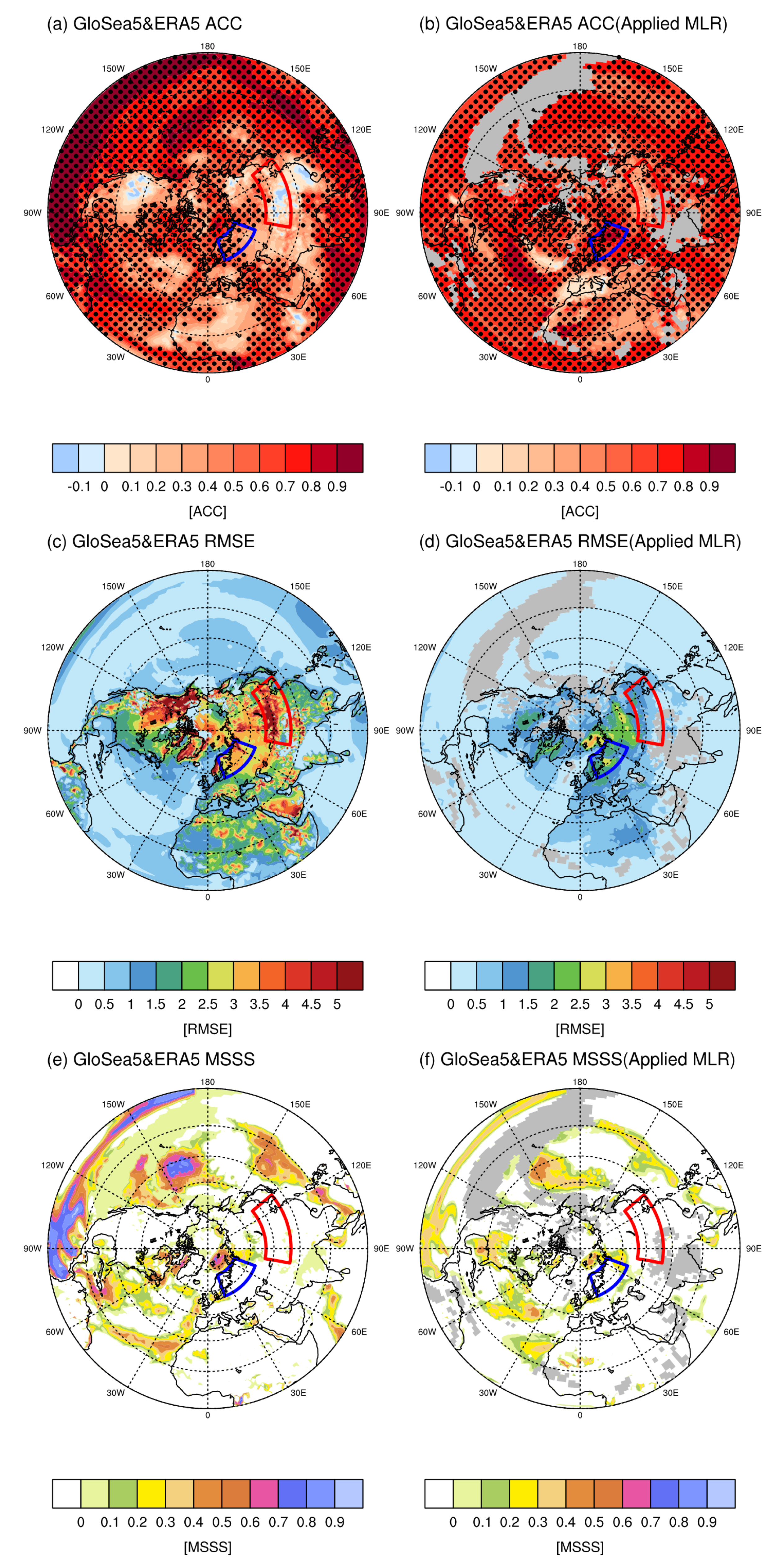
Statistical skill scores were applied to verify deterministic prediction skills: the simple anomaly correlation coefficient (ACC) and the mean-square skill score (MSSS) [38,39]. To calculate ACC and MSSS, we used the following equation (Equation (6)):
A C C τ = j = 1 k F j τ F ¯ τ O j τ O ¯ τ j = 1 k F j τ F ¯ τ 2 j = 1 k O j τ O ¯ τ 2
The ACC represents the linear correlation between the predicted value and the observed value (reanalysis products) and has a value ranging from −1 to 1; therefore, the closer it is to 1, the more accurate the interpretation of the observed value phase. The ACC calculates the correlation coefficients between a set of forecast runs F and observation O , where O corresponds to the ERA5 reanalysis product in this study. Forecast ensembles can be characterized by F j τ , where F is the ensemble mean prediction in each model, j is the initialization year, k is the hindcast period of the model experiments, and τ is the forecast lead-time. The climatological averages of reanalysis products and forecast runs are calculated by the following formula (Equation (7)):
O ¯ τ = 1 k j = 1 k O j τ   and   F ¯ τ = 1 k j = 1 k F j τ
MSSS is based on the MSE [40], which is calculated as
M S E F τ = 1 n j = 1 n F j τ F ¯ τ O j τ O ¯ τ ,   M S E O ¯ τ = 1 n j = 1 n O j τ O ¯ τ 2
M S S S τ = 1 M S E F τ M S E O ¯ τ = A C C τ 2 A C C τ s τ F s τ O 2
s τ F 2 = 1 n j = 1 n F j τ F ¯ τ 2 ,       s τ O 2 = M S E O ¯ τ = 1 n j = 1 n O j τ O ¯ t 2
The MSSS was used to evaluate the prediction model based on the observed value size and consisted of terms of the MSE (Equation (8)). The calculation of MSSS is a function of ACC and the predicted-to-value observed variance ratio s τ F / s τ O as in Equation (9) (detailed denotation of each term in Equation (9) is in Equation (10)). In particular, the expression in parentheses (ACC(τ) − s τ F / s τ O ) considering the variance ratio between prediction and observation is called ‘conditional bias’. Conditional bias is a different concept from ‘mean bias’ and can exist when the magnitude of the trend over time is different, even if the means of observation and prediction are the same. The MSSS value ranged from negative infinity to 1. The predictability is evaluated as good when it approaches 1, which means that the MSE is closer to zero.
In the statistical skills, the ACC cannot predict the fluctuation, only its phase; however, the MSSS compensates for the disadvantage that the existing ACC does not consider the difference in variance between the observation and model. In addition, in the literature, subjective threshold values are empirically used for evaluating statistical skill-score results (i.e., ACC greater than approximately 0.6 and MSSS greater than 0) [39,41,42].

3. Results

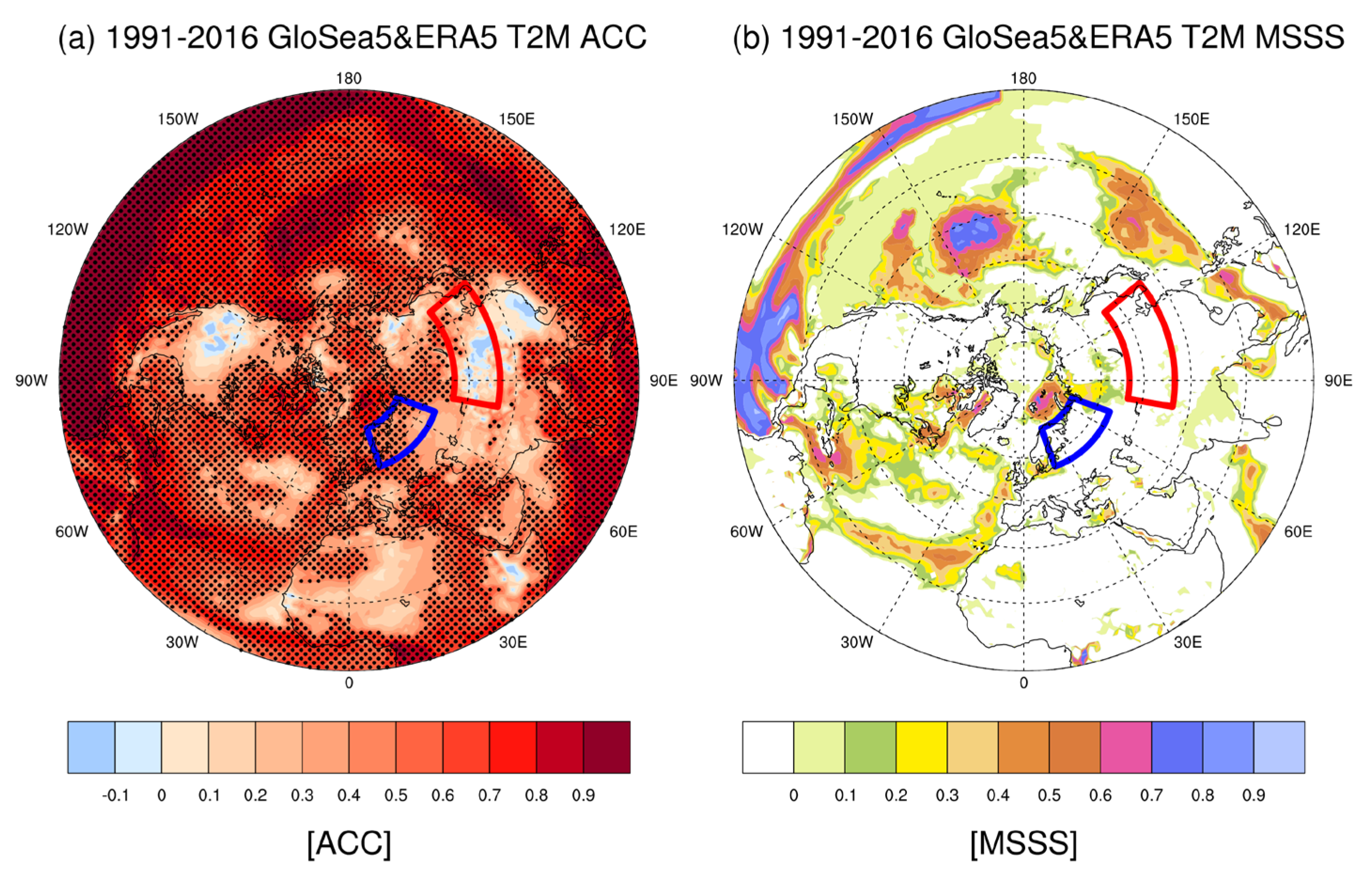
3.1. The Predictability Evaluation in Wintertime T2m of GloSea5

We examined the spatial distribution of the seasonal forecast skill of the GloSea5 model using two skill-score tests. The seasonal prediction skill of the GloSea5 model was evaluated from 1991 to 2016 based on its ability to predict the boreal winter T2m. This was compared with the ERA5 reanalysis data.
As shown in Figure 1a, the GloSea5 model has an ACC score of 0.6 or more in most ocean areas and the Arctic region, partly caused by the long-term memory effect of the ocean and sea ice. Noticeably, ACC suddenly drops to almost zero over most continental regions such as North America, East Asia (red box), and Northern Africa, except for Northern Europe (blue box), which shows above 0.6 in the ACC score. However, the MSSS for Northern Europe (blue box) in Figure 1b is almost zero, which implies that the GloSea5 model tends to predict the phase of variability in Northern Europe accurately but does not perform well when it comes to predicting the magnitude of variability. In contrast, Figure 1b shows that the MSSS at sea surface air temperature, where the temporal memory of the initial condition was maintained, exhibited a significant value.

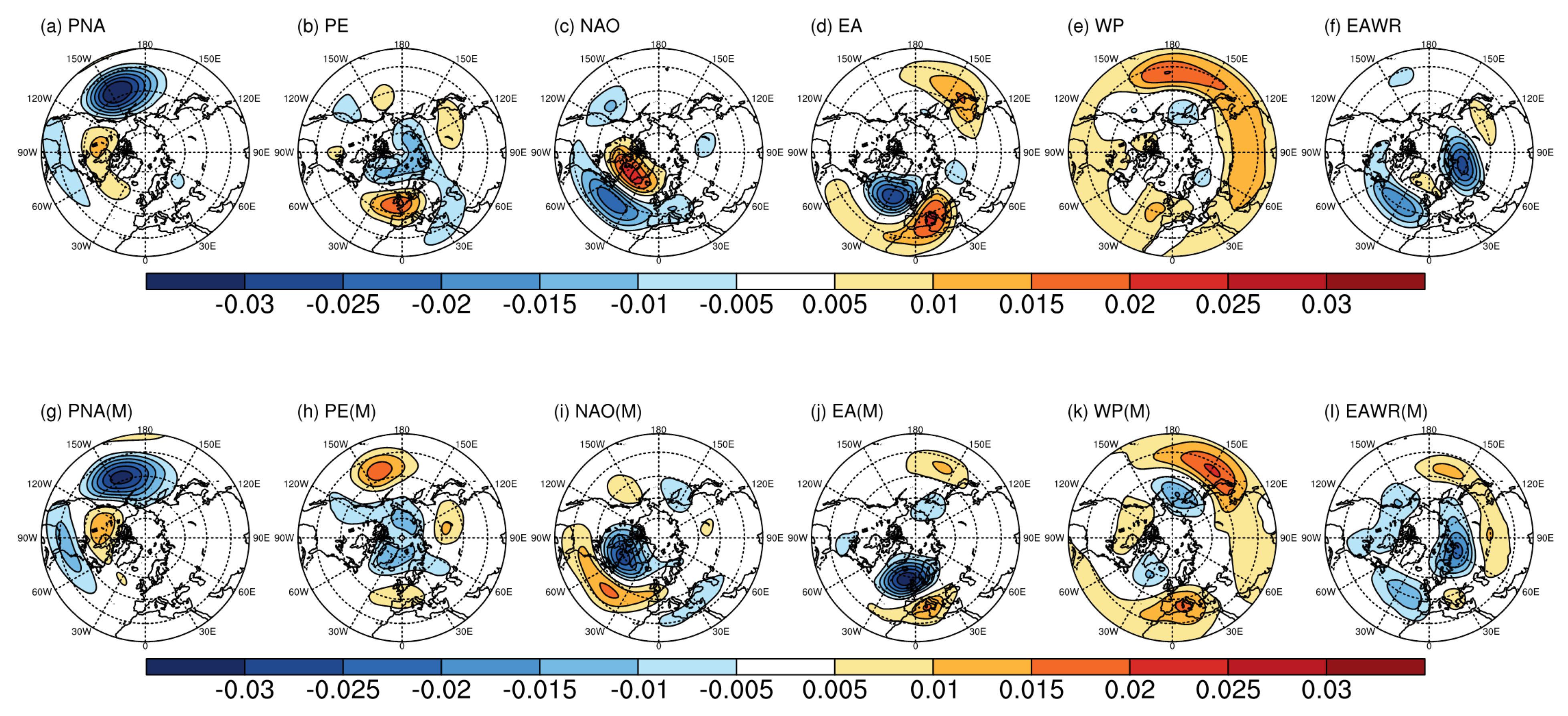
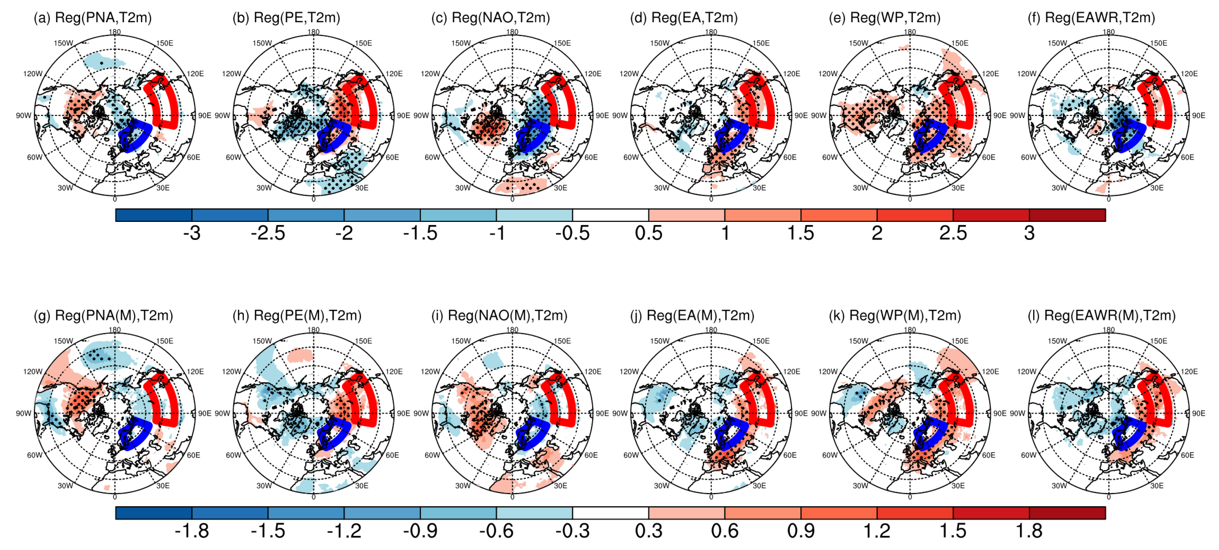
3.2. Predictability Evaluation in Teleconnection Patterns of GloSea5

Climate has many nonlinearities. Therefore, reducing nonlinearity and identifying important patterns that explain variability are imperative. The EOF is well known for extracting important patterns from atmospheric fluctuations. Calculating n modes in the EOF analysis yields the spatial field of n eigenvectors (teleconnection patterns) and time series of n principal components. Considering the orthogonal nature of the data, the original data were computed based on the dot product of the spatial field eigenvectors and the principal component (PC) time series. Because of the disadvantage that EOF is orthogonal in time and space, regional patterns can be identified through REOF using ‘varimax’ rotation [43]. The northern hemisphere region (20–90° N) geopotential height anomaly at 500 hPa is calculated as an EOF mode, and the mode complexity is minimized by taking a ‘varimax’ rotation that maximizes the variance of each mode.
Therefore, patterns such as EAWR, PE, and SCAND, which could not be devised in EOF, can be derived [44]. We derived winter teleconnection patterns using the REOF method for the ERA5 reanalysis data. Specific teleconnection patterns were defined by calculating the correlation coefficient between the PC time series of ERA5 and the PC time series of each teleconnection pattern provided by NOAA/CPC (https://www.cpc.ncep.noaa.gov/data/teledoc/telecontents.shtml, accessed on 6 January 2023). Based on defined teleconnection patterns from the ERA5 reanalysis data, the GloSea5 model was used to determine the accuracy of each teleconnection pattern during the northern hemisphere winter season (December–January–February).
Figure 2 shows six dominant teleconnection patterns that can be observed in the boreal winter season of ERA5 reanalysis data: NAO, East Atlantic (EA), East Atlantic/Western Russia (EAWR), PE, West Pacific (WP), and PNA patterns.
The PNA pattern shows negative anomaly centers in the North Pacific and Southeastern United States (US) and positive anomaly centers in Canada (Figure 2a). In the PE pattern (Figure 2b), a negative anomaly center was located in the polar region, and a positive anomaly center was located in the northern area of China. The NAO pattern consists of two dipole anomalies centers in Greenland and the North Atlantic (Figure 2c). The EA pattern is similar to the NAO pattern but shows an anomaly center skewed to the east (Figure 2d). In the WP pattern, the negative anomaly was located on the Kamchatka Peninsula, and the positive anomaly center was located east to west in the North Pacific region (Figure 2e). Four anomalies centers in the EAWR pattern (Figure 2f) affect Eurasia. A positive anomaly center is located in Northern Europe, whereas a negative anomaly center is located in the North Atlantic and Russia.
Seven teleconnection patterns, including the SCAND pattern, can be observed in the northern hemisphere during winter. However, the GloSea5 model did not exhibit a significant SCAND pattern. Therefore, the SCAND pattern was excluded from the analysis. Consequently, the GloSea5 model showed an average pattern correlation coefficient (PCC) of 0.78 for the teleconnection patterns (excluding SCAND patterns) calculated from the reanalysis data (see Figure 2g–l). In particular, the GloSea5 model provided an excellent simulation of the PNA pattern (average PCC value of 0.92). The EA pattern had the lowest correlation values among all teleconnection patterns in GloSea5 (average PCC value of 0.71) (Table 2). Consequently, the GloSea5 model generally has a high simulation capability for teleconnection patterns.
All teleconnection patterns occurring in the boreal winter were highly correlated with T2m anomalies over North America and East Asia. The PNA pattern showed a cold trend in the Arctic region and a warm trend in North America (Figure 3a). However, the GloSea5 model only showed a warm trend in North America (Figure 3g). In the PE pattern, the Arctic region exhibits a cold trend, whereas Northern Europe and East Asia exhibit a warm trend (Figure 3b). A similar trend was also observed in the GloSea5 model and reanalysis data (Figure 3h). In the NAO pattern, Greenland has warm and cold trends in Northern Europe and East Asia (Figure 3c). Although GloSea5 and the reanalysis data show similar trends, the magnitude is weaker over Northern Europe, and East Asia and North America have a stronger warm trend (Figure 3i). The GloSea5 model and reanalysis data indicate that the warming trend of the EA pattern is strongly correlated with Western Europe and the Korean Peninsula (Figure 3d,j). The WP pattern showed a warming trend over the entire continent, especially in North America, Europe, Eurasia, and East Asia (Figure 3e,k). As seen from the EAWR pattern, the Barents Sea and adjacent continental regions show a cold trend, whereas East Asia displays a warm trend (Figure 3f). In the GloSea5 model, the EAWR pattern was highly related not only to East Asia but also to East Asia and Northern Europe (Figure 3l). The most prevalent teleconnection patterns were PE, EA, and WP in East Asia. As with the PNA pattern, T2m in North America was highly correlated with these patterns.
As a result, the EA and WP patterns, showing a broad, warm trend over East Asia, were similarly simulated in the reanalysis data and the GloSea5 model. Although GloSea5 simulated a weaker trend than the reanalysis data, the overall trends were similar. Therefore, in the case of the GloSea5 model, the capability of predicting T2m using teleconnection patterns can be considered by applying the MLR model.

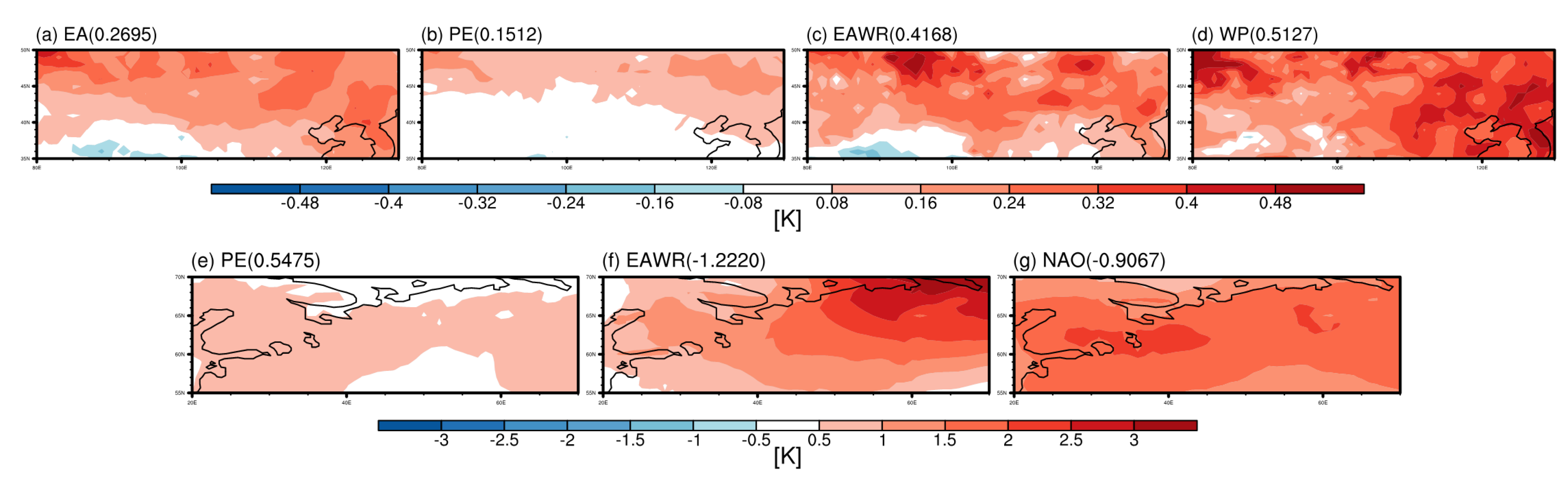
3.3. Improved Predictions over T2m by Statistical Prediction Model of the Teleconnection Patterns

In Section 3.1, we confirmed that the GloSea5 model shows relatively low predictability of T2m over the continental region. A statistical model based on the MLR model was developed using the GloSea5 model’s reliable simulation performance on teleconnection patterns to reduce the uncertainty of T2m in East Asia.
Section 3.2 also noted that different regions are affected by different teleconnection patterns. Significant teleconnection patterns were identified through the correlation between the index for each teleconnection pattern and the time series of T2m anomaly. Table 3 shows the correlation coefficients between each teleconnection pattern’s PC time series (each mode and PC time series obtained by the REOF method) and the area-averaged time series of T2m anomalies in East Asia and Northern Europe. Furthermore, we found that T2m in East Asia was influenced by the EA, PE, EAWR, and WP patterns. The PE, EAWR, and NAO patterns were strongly related to T2m in Northern Europe. Using the indices of teleconnection patterns as predictors of the MLR model described in Section 2.2, the following MLR equations were found to have the highest performance in East Asia and Northern Europe.
Y E a s t   A s i a = 0 + 0.2695 X E A + 0.1512 X P E + 0.4168 X E A W R + 0.5127 X W P
Y N o r t h e r n   E u r o p e = 0 + 0.5475 X P E 1.2220 X E A W R 0.9067 X N A O
In the MLR equations (Equations (11) and (12)), each coefficient represents a linear regression coefficient between the teleconnection pattern and T2m anomalies. The coefficient value indicates the regression equation’s contribution to each teleconnection pattern to the prediction of T2m. Therefore, we can interpret that the higher coefficients contribute more to predicted T2m in the MLR model. Positive WP and EAWR patterns strongly affected T2m in East Asia (Figure 4c,d). In Northern Europe, T2m was also influenced by negative EAWR and NAO patterns (Figure 4e,g).
The predictability of T2m using the MLR model was directly compared to that obtained from the GloSea5 model forecast (Figure 5). As a prerequisite for the MLR model, more than two significant teleconnection patterns must exist in the target region. Therefore, parts of continental regions and the Pacific Ocean with fewer than two members are indicated by a gray area (a missing value) in Figure 5b,d,f.
In Figure 5a, the T2m ACC of the GloSea5 model has predictability close to 0 in North America, Eurasia, East Asia, and the African continent (with negative values in the limited North American and Eurasian regions). In North America and East Asia, the ACC of T2m applied with the MRL appeared at a significance level of 95% (Figure 5b). In addition, the score on the northern hemisphere continents, where the RMSE had a score of 5 or higher, was significantly improved as a result of lowering to an average score of 1 (Figure 5b,d). In particular, it can be found that the RMSE improvement in Alaska and East Asia is remarkable (Figure 5b). Because ACC is normalized, evaluating the magnitude of variability is impossible. To compensate for this limitation, MSSS was used to assess the magnitude of predictability. However, the value of MSSS, which had a negative infinity for GloSea5, showed a slight difference in predictability improvement in the value of MSSS to which MRL was applied (Figure 5f).
However, the value of MSSS, which had a negative infinity of GloSea5, showed a slight difference in the predictability improvement in the value of MSSS to which MRL was applied. This was improved in East Asia and Northern Europe (Table 4). Compared to the GloSea5 model, the ACC score of the GloSea5 model to which the MLR model was applied increased by 0.25 in East Asia and 0.33 in Northern Europe. The reduction in error reduced the RMSE score by −0.63 in East Asia and −0.68 in Northern Europe. MSSS slightly increased by −0.09 in Northern Europe but slightly decreased by +0.37 compared to the GloSea5 model in East Asia. When ACC is statistically significant, but MSSS is not significant, it means that the phase of fluctuation is predicted well, but the predictability of the magnitude of fluctuation is low. Therefore, in the case of MSSS, this is not a significant improvement, but it means that the predictability of the fluctuation is also improved through the MLR equation.

4. Discussion

In general, pronounced teleconnection patterns explain large variances in climate variability, and recent climate models have tended to capture major teleconnection patterns quite well. Based on this, we devised a method to enhance the predictability of the seasonal forecast model, especially for regions where the T2m prediction skill is not useful.
In this study, we suggest an enhanced forecast skill of winter temperature of specific domains using teleconnection patterns simulated by the GloSea5 seasonal prediction model. In particular, we applied teleconnection patterns as predictors in a MLR model to improve the GloSea5 model. The GloSea5 model exhibited less skill in predicting T2m in the East Asia region. We focused on the fact that the T2m in East Asia is affected by specific teleconnection patterns such as the EA, PE, EAWR, and WP patterns. Exploiting the reasonable prediction skills of Glosea5 for these teleconnection modes, we constructed an MLR model to predict the T2m over East Asia using teleconnection patterns as predictors. The devised MLR model successfully increased the predictability of the T2m over East Asia compared with the prediction results from the dynamic seasonal forecast model. In particular, predictability has been greatly improved not only in East Asia, where the dynamic predictability of the GloSea5 model is low, but also on the continents of the northern hemisphere. Although applicable not only in winter but also in other seasons, such as summer, the East Asia region is more affected, such as by the Circumglobal Teleconnection (CGT) or Pacific–Japan (PJ) teleconnections in summer [45]. Therefore, it is important to set predictors according to the season and analysis region suitable for predictive improvement.
Our results suggest that applying a well-designed statistical model to the output of the seasonal prediction model can efficiently improve the quality of seasonal forecasts. The method devised in this study can be applied to any physical variable, such as humidity and precipitation, which are related to specific teleconnection patterns but typically show low predictability. We plan to extend this possibility in future studies.

5. Conclusions and Policy Implication

This study proposed a statistical model to improve T2m predictability in continental regions in winter by examining the linear relationship between teleconnection patterns and T2m anomaly. The usefulness of the statistical method for improving predictability using the MLR model was verified using hindcast data from the GloSea5 model. As a result, it was confirmed that the predictability was improved not only in the T2m of East Asia but also in the entire northern hemisphere continental region. It is possible to improve the predictability of other climatic variables (precipitation, wind, SST) other than T2m by using an MLR model. Our research implies a solution that computational issues, which require enormous resources in operational prediction systems, can be efficiently improved through statistical approaches. Therefore, further research in this direction will help to establish climate-related policies based on accurate forecasts amid increasing damage from extreme climates.

Author Contributions

Y.L. conducted the analyses and took the lead in writing the paper. H.-R.K. guided the data analysis and wrote the paper. N.N. discussed and interpreted the data and methodology. K.-Y.K. provided feedback for this paper. B.-M.K. worked on the idea and the hypothesis, and helped shaped the research. All authors have read and agreed to the published version of the manuscript.

Funding

This research was funded by the Korea Meteorological Administration Research and Development Program under Grant (KMI2022-01110). It was also supported by Basic Science Research Program through the National Research Foundation of Korea (NRF) funded by the Ministry of Education (2018R1A6A1A08025520), and the National Research Foundation of Korea (NRF) grant funded by the Korea government (MSIT) (2021R1A2C1093402).

Data Availability Statement

The seasonal indices of teleconnection patterns data are provided by the CPC website (https://www.cpc.ncep.noaa.gov/data/teledoc/telecontents.shtml, accessed on 6 January 2023), and the ERA5 dataset used has been acquired from the ECMWF archive (https://www.ecmwf.int/en/forecasts/dataset/ecmwf-reanalysis-v5, accessed on 6 January 2023). The GloSea5 data that support the findings of this study are available upon reasonable request from the authors.

Acknowledgments

This research was funded by the Korea Meteorological Administration Research and Development Program under Grant (KMI2022-01110). This research was also supported by Basic Science Research Program through the National Research Foundation of Korea (NRF) funded by the Ministry of Education (2018R1A6A1A08025520), and the National Research Foundation of Korea (NRF) grant funded by the Korea government (MSIT) (2021R1A2C1093402).

Conflicts of Interest

The authors declare no conflict of interest.

References

  1. Gu, H.; Yan, W.; Elahi, E.; Cao, Y. Air pollution risks human mental health: An implication of two-stages least squares estimation of interaction effects. Environ. Sci. Pollut. Res. 2020, 27, 2036–2043. [Google Scholar] [CrossRef] [PubMed]
  2. Elahi, E.; Khalid, Z.; Tauni, M.Z.; Zhang, H.; Lirong, X. Extreme weather events risk to crop-production and the adaptation of innovative management strategies to mitigate the risk: A retrospective survey of rural Punjab, Pakistan. Technovation 2022, 117, 102255. [Google Scholar] [CrossRef]
  3. Lorenz, E.N. Atmospheric predictability experiments with a large numerical model. Tellus A Dyn. Meteorol. Oceanogr. 1982, 34, 505–513. [Google Scholar] [CrossRef]
  4. Palmer, T. Predicting uncertainty in forecasts of weather and climate. Rep. Prog. Phys. 2000, 63, 71–116. [Google Scholar] [CrossRef] [Green Version]
  5. Slingo, J.; Palmer, T. Uncertainty in weather and climate prediction. Philos. Trans. R. Soc. A Math. Phys. Eng. Sci. 2011, 369, 4751–4767. [Google Scholar] [CrossRef] [PubMed]
  6. Guo, Z.; Dirmeyer, P.A.; DelSole, T. Land surface impacts on subseasonal and seasonal predictability. Geophys. Res. Lett. 2011, 38, L24812. [Google Scholar] [CrossRef]
  7. Kim, H.-M.; Webster, P.J.; Curry, J.A. Seasonal prediction skill of ECMWF System 4 and NCEP CFSv2 retrospective forecast for the Northern Hemisphere Winter. Clim. Dyn. 2012, 39, 2957–2973. [Google Scholar] [CrossRef] [Green Version]
  8. Krishnamurthy, V. Predictability of Weather and Climate. Earth Space Sci. 2019, 6, 1043–1056. [Google Scholar] [CrossRef] [Green Version]
  9. Tian, B.; Fan, K.; Yang, H. East Asian winter monsoon forecasting schemes based on the NCEP’s climate forecast system. Clim. Dyn. 2017, 51, 2793–2805. [Google Scholar] [CrossRef]
  10. Pokhrel, S.; Hazra, A.; Chaudhari, H.S.; Saha, S.K.; Paulose, F.; Krishna, S.; Krishna, P.M.; Rao, S.A. Hindcast skill improvement in Climate Forecast System (CFSv2) using modified cloud scheme. Int. J. Clim. 2018, 38, 2994–3012. [Google Scholar] [CrossRef]
  11. Dai, H.; Fan, K. Skilful two-month-leading hybrid climate prediction for winter temperature over China. Int. J. Clim. 2020, 40, 4922–4943. [Google Scholar] [CrossRef]
  12. Luo, X.; Wang, B. How predictable is the winter extremely cold days over temperate East Asia? Clim. Dyn. 2017, 48, 2557–2568. [Google Scholar] [CrossRef]
  13. Wang, L.; Ting, M.; Kushner, P.J. A robust empirical seasonal prediction of winter NAO and surface climate. Sci. Rep. 2017, 7, 279. [Google Scholar] [CrossRef] [PubMed] [Green Version]
  14. Hall, R.J.; Scaife, A.A.; Hanna, E.; Jones, J.M.; Erdélyi, R. Simple Statistical Probabilistic Forecasts of the Winter NAO. Weather. Forecast 2017, 32, 1585–1601. [Google Scholar] [CrossRef] [Green Version]
  15. Golian, S.; Murphy, C.; Wilby, R.L.; Matthews, T.; Donegan, S.; Quinn, D.F.; Harrigan, S. Dynamical–statistical seasonal forecasts of winter and summer precipitation for the Island of Ireland. Int. J. Clim. 2022, 42, 5714–5731. [Google Scholar] [CrossRef]
  16. Rust, H.W.; Richling, A.; Bissolli, P.; Ulbrich, U. Linking teleconnection patterns to European temperature—A multiple linear regression model. Meteorol. Z. 2015, 24, 411–423. [Google Scholar] [CrossRef]
  17. MacLachlan, C.; Arribas, A.; Peterson, K.A.; Maidens, A.; Fereday, D.; Scaife, A.A.; Gordon, M.; Vellinga, M.; Williams, A.; Comer, R.E.; et al. Global Seasonal forecast system version 5 (GloSea5): A high-resolution seasonal forecast system. Q. J. R. Meteorol. Soc. 2015, 141, 1072–1084. [Google Scholar] [CrossRef]
  18. Lim, Y.-K.; Kim, H.-D. Comparison of the impact of the Arctic Oscillation and Eurasian teleconnection on interannual variation in East Asian winter temperatures and monsoon. Theor. Appl. Clim. 2015, 124, 267–279. [Google Scholar] [CrossRef]
  19. Wang, B.; Lee, J.-Y.; Kang, I.-S.; Shukla, J.; Park, C.-K.; Kumar, A.; Schemm, J.; Cocke, S.; Kug, J.-S.; Luo, J.-J.; et al. Advance and prospectus of seasonal prediction: Assessment of the APCC/CliPAS 14-model ensemble retrospective seasonal prediction (1980–2004). Clim. Dyn. 2009, 33, 93–117. [Google Scholar] [CrossRef] [Green Version]
  20. Gao, Z.; Hu, Z.-Z.; Jha, B.; Yang, S.; Zhu, J.; Shen, B.; Zhang, R. Variability and predictability of Northeast China climate during 1948–2012. Clim. Dyn. 2014, 43, 787–804. [Google Scholar] [CrossRef]
  21. Jung, M.-I.; Son, S.-W.; Choi, J.; Kang, H.-S. Assessment of 6-Month Lead Prediction Skill of the GloSea5 Hindcast Experiment. Atmosphere 2015, 25, 323–337. [Google Scholar] [CrossRef] [Green Version]
  22. Park, H.-J.; Ahn, J.-B. Combined effect of the Arctic Oscillation and the Western Pacific pattern on East Asia winter temperature. Clim. Dyn. 2015, 46, 3205–3221. [Google Scholar] [CrossRef] [Green Version]
  23. Lim, Y.-K.; Kim, H.-D. Impact of the dominant large-scale teleconnections on winter temperature variability over East Asia. J. Geophys. Res. Atmos. 2013, 118, 7835–7848. [Google Scholar] [CrossRef] [Green Version]
  24. Liu, Y.; Wang, L.; Zhou, W.; Chen, W. Three Eurasian teleconnection patterns: Spatial structures, temporal variability, and associated winter climate anomalies. Clim. Dyn. 2014, 42, 2817–2839. [Google Scholar] [CrossRef]
  25. Gao, T.; Yu, J.-Y.; Paek, H. Impacts of four northern-hemisphere teleconnection patterns on atmospheric circulations over Eurasia and the Pacific. Theor. Appl. Clim. 2016, 129, 815–831. [Google Scholar] [CrossRef] [Green Version]
  26. Walters, D.N.; Best, M.J.; Bushell, A.C.; Copsey, D.; Edwards, J.M.; Falloon, P.D.; Harris, C.M.; Lock, A.P.; Manners, J.C.; Morcrette, C.J.; et al. The Met Office Unified Model Global Atmosphere 3.0/3.1 and JULES Global Land 3.0/3.1 configurations. Geosci. Model Dev. 2011, 4, 919–941. [Google Scholar] [CrossRef] [Green Version]
  27. Brown, A.; Milton, S.; Cullen, M.; Golding, B.; Mitchell, J.F.B.; Shelly, A. Unified Modeling and Prediction of Weather and Climate: A 25-Year Journey. Bull. Am. Meteorol. Soc. 2012, 93, 1865–1877. [Google Scholar] [CrossRef]
  28. Madec, G.; Bourdallé-Badie, R.; Bouttier, P.-A.; Bricaud, C.; Bruciaferri, D.; Calvert, D.; Chanut, J.; Clementi, E.; Coward, A.; Delrosso, D.; et al. NEMO Ocean Engine Gurvan Madec, and the NEMO Team; Notes du Pôle de modélisation de l’Institut Pierre-Simon Laplace; IPSL: Portland, OR, USA, 2016; Volume 27, ISSN 1288-1619. [Google Scholar]
  29. Best, M.J.; Pryor, M.; Clark, D.B.; Rooney, G.G.; Essery, R.L.H.; Ménard, C.B.; Edwards, J.M.; Hendry, M.A.; Porson, A.; Gedney, N.; et al. The Joint UK Land Environment Simulator (JULES), model description–Part 1: Energy and water fluxes. Geosci. Model Dev. 2011, 4, 677–699. [Google Scholar] [CrossRef] [Green Version]
  30. Hunke, E.C.; Lipscomb, W.H.; Turner, A.K.; Jeffery, N.; Elliott, S. CICE: The Los Alamos Sea Ice Model Documentation and Software User’s Manual Version 4.1 LA-CC-06-012. Fluid Dyn. Group Los Alamos Natl. Lab. 2010, 675, 500. [Google Scholar]
  31. Valcke, S. The OASIS3 coupler: A European climate modelling community software. Geosci. Model Dev. 2013, 6, 373–388. [Google Scholar] [CrossRef] [Green Version]
  32. Lea, D.J.; Mirouze, I.; Martin, M.J.; King, R.R.; Hines, A.; Walters, D.; Thurlow, M. Assessing a New Coupled Data Assimilation System Based on the Met Office Coupled Atmosphere–Land–Ocean–Sea Ice Model. Mon. Weather. Rev. 2015, 143, 4678–4694. [Google Scholar] [CrossRef]
  33. Hersbach, H.; Bell, B.; Berrisford, P.; Hirahara, S.; Horanyi, A.; Muñoz-Sabater, J.; Nicolas, J.; Peubey, C.; Radu, R.; Schepers, D.; et al. The ERA5 global reanalysis. Q. J. R. Meteorol. Soc. 2020, 146, 1999–2049. [Google Scholar] [CrossRef]
  34. Heo, S.-I.; Hyun, Y.-K.; Ryu, Y.; Kang, H.-S.; Lim, Y.-J.; Kim, Y. An Assessment of Applicability of Heat Waves Using Extreme Forecast Index in KMA Climate Prediction System (GloSea5). Atmos. Korean Meteorol. Soc. 2019, 29, 257–267. [Google Scholar] [CrossRef]
  35. Uyanık, G.K.; Güler, N. A Study on Multiple Linear Regression Analysis. Procedia-Soc. Behav. Sci. 2013, 106, 234–240. [Google Scholar] [CrossRef] [Green Version]
  36. Salmerón, R.; García, C.B.; García, J. Variance Inflation Factor and Condition Number in multiple linear regression. J. Stat. Comput. Simul. 2018, 88, 2365–2384. [Google Scholar] [CrossRef]
  37. Berrar, D. Cross-Validation. In Encyclopedia of Bioinformatics and Computational Biology: ABC of Bioinformatics; Elsevier: Amsterdam, The Netherlands, 2018; Volumes 1–3, pp. 542–545. ISBN 9780128114322. [Google Scholar]
  38. Goddard, L.; Kumar, A.; Solomon, A.; Smith, D.; Boer, G.; Gonzalez, P.; Kharin, V.; Merryfield, W.; Deser, C.; Mason, S.J.; et al. A verification framework for interannual-to-decadal predictions experiments. Clim. Dyn. 2012, 40, 245–272. [Google Scholar] [CrossRef] [Green Version]
  39. Choi, J.; Son, S.-W.; Ham, Y.-G.; Lee, J.-Y.; Kim, H.-M. Seasonal-to-Interannual Prediction Skills of Near-Surface Air Temperature in the CMIP5 Decadal Hindcast Experiments. J. Clim. 2016, 29, 1511–1527. [Google Scholar] [CrossRef]
  40. Allan, H. Murphy Skill Scores Based on the Mean Square Error and Their Relationships to the Correlation Coefficient. Mon. Weather. Rev. 1988, 116, 2417–2424. [Google Scholar] [CrossRef]
  41. Lin, H.; Brunet, G.; Derome, J. Forecast Skill of the Madden–Julian Oscillation in Two Canadian Atmospheric Models. Mon. Weather. Rev. 2008, 136, 4130–4149. [Google Scholar] [CrossRef]
  42. Chevuturi, A.; Turner, A.G.; Johnson, S.; Weisheimer, A.; Shonk, J.K.P.; Stockdale, T.N.; Senan, R. Forecast skill of the Indian monsoon and its onset in the ECMWF seasonal forecasting system 5 (SEAS5). Clim. Dyn. 2021, 56, 2941–2957. [Google Scholar] [CrossRef]
  43. Hannachi, A.; Jolliffe, I.T.; Stephenson, D.B. Empirical orthogonal functions and related techniques in atmospheric science: A review. Int. J. Clim. 2007, 27, 1119–1152. [Google Scholar] [CrossRef]
  44. Handorf, D.; Dethloff, K. How well do state-of-the-art atmosphere-ocean general circulation models reproduce atmospheric teleconnection patterns? Tellus A Dyn. Meteorol. Oceanogr. 2012, 64, 19777. [Google Scholar] [CrossRef] [Green Version]
  45. Lee, K.-J.; Kwon, M.; Kang, H.-W.; Author, C. Record-Breaking High Temperature in July 2021 over East Sea and Possible Mechanism. Atmos. Korean Meteorol. Soc. 2022, 32, 17–25. [Google Scholar] [CrossRef]
Figure 1. GloSea5 hindcast experiments were evaluated against ERA5 data. (a) Anomaly correlation coefficient (ACC) and (b) mean-squared skill score (MSSS) from December to February (DJF mean) of 1991–2016 for surface temperature (T2m). Blue and red boxes indicate the areas of Northern Europe and East Asia, respectively. The black dots indicate statistical significance at the 95% confidence level.
Atmosphere 14 00438 g001
Figure 2. Teleconnection patterns of northern hemispheric (20–90° N) 500 hPa geopotential height (Z500) anomalies using ERA5 reanalysis products for (a) PNA (Pacific/North American), (b) PE (Polar/Eurasia), (c) NAO (North Atlantic Oscillation), (d) EA (East Atlantic), (e) WP (West Pacific), and (f) EAWR (East Atlantic/Western Russia) (Top). (gl) are the teleconnection patterns of the GloSea5 (M) model (Bottom). The (M) denotes the GloSea5 model.
Atmosphere 14 00438 g002
Figure 3. The spatial distribution of surface temperature anomalies (T2m, K) regressed on the positive teleconnection pattern (‘negative’ surface temperature when the centers of the teleconnection pattern of Fig2 have opposite signs) of geopotential height anomalies at 500 hPa (Z500, gpm) during boreal winter (DJF mean) from 1979 to 2019 using ERA5 reanalysis (af) (Top). (gl) are the T2m anomalies of the GloSea5 (M) model (Bottom). Denote (M) is the GloSea5 model. Blue and red boxes indicate the areas of Northern Europe and East Asia, respectively. The black dots indicate statistical significance at the 95% confidence level.
Atmosphere 14 00438 g003
Figure 4. The spatial distribution of surface temperature (T2m, K) regressed on the principal component (PC) time series of the most related teleconnection patterns to the East Asia (EA) domain (ad). Image (eg) are the same as (ad), except they are for the Northern Europe (NE) domain. The coefficient of the predictor for each related teleconnection pattern determined by the MLR model is in parentheses.
Atmosphere 14 00438 g004
Figure 5. The spatial distribution of surface temperature (T2m, K) between the ERA5 data and GloSea5 hindcast during boreal wintertime (DJF) from 1979 to 2019. The left side is for the GloSea5 model (a,c,e), and the right is for the GloSea5 model with the MLR model (applied MLR) (b,d,f). Top: Anomaly correlation coefficient (ACC); Mid: Root mean square error (RMSE); Bottom; Mean-squared skill score (MSSS). The blue and red boxes indicate the areas of East Asia and Northern Europe, respectively. The black dots indicate statistical significance at the 95% confidence level.
Atmosphere 14 00438 g005
Table 1. Reference for information of the ERA5 (ECMWF Reanalysis 5th Generation) and the GloSea5 (Global Seasonal Forecast System version 5) seasonal prediction models referred to within the text.
Reanalysis DataERA5
InstituteECMWF
Period1979–2019 (41 years)
Resolution0.25° × 0.25° (interpolated at 1° intervals)
Variables500 hPa geopotential height (Z500, gpm),
surface temperature (T2m, K)
Model DataGloSea5
InstituteKMA
Period1991–2016 (26 years)
Number of ensembles3-ensemble members
Resolution0.83° × 0.56° (interpolated at 1° intervals)
Variables500 hPa geopotential height (Z500, gpm),
surface temperature (T2m, K)
Table 2. Pattern correlation coefficient (PCC) of six teleconnection patterns between the GloSea5 model and ERA5 reanalysis data.
PNAPENAOEAWPEAWR
Pattern Corr.0.920.740.820.710.750.73
Table 3. The correlation coefficient between the PC time series of each teleconnection pattern and surface temperature (T2m) in East Asia (EA) and Northern Europe (NE) (an asterisk (*) indicates the statistical significance at the 95% confidence level).
PNAPENAOEAWPEAWR
EA (East Asia)−0.10.48 *−0.30.59 *0.54 *0.43 *
NE (Northern Europe)−0.20.5 *−0.75 *0.260.23−0.39 *
Table 4. Correlation coefficients for the GloSea5 model (before) and applied MLR of the GloSea5 model (after) (compared to the ERA5) in East Asia and Northern Europe.
BeforeAfter (Applied MLR)
ACCRMSEMSSSACCRMSEMSSS
EA (East Asia)0.191.37−6.080.44 (+0.25)0.74 (−0.63)−5.71 (+0.37)
NE (Northern Europe)0.422.07−0.600.75 (+0.33)1.39 (−0.68)−0.69 (−0.09)
Disclaimer/Publisher’s Note: The statements, opinions and data contained in all publications are solely those of the individual author(s) and contributor(s) and not of MDPI and/or the editor(s). MDPI and/or the editor(s) disclaim responsibility for any injury to people or property resulting from any ideas, methods, instructions or products referred to in the content.

