Article

Exploring Natural and Anthropogenic Drivers of PM2.5 Concentrations Based on Random Forest Model: Beijing–Tianjin–Hebei Urban Agglomeration, China

1
National Engineering Research Center of Building Technology, Beijing 100013, China
2
China Academy of Building Research, Beijing 100013, China
3
Beijing Academy of Science and Technology, Beijing 100089, China
4
Institute of Geographic Sciences and Natural Resources Research, Chinese Academy of Sciences, Beijing 100101, China
5
College of Resource and Environment, University of Chinese Academy of Sciences, Beijing 100049, China
*
Author to whom correspondence should be addressed.
Atmosphere 2023, 14(2), 381; https://doi.org/10.3390/atmos14020381
Submission received: 6 January 2023 / Revised: 4 February 2023 / Accepted: 13 February 2023 / Published: 15 February 2023
(This article belongs to the Special Issue Air Quality in Metropolitan Areas and Megacities)

Abstract

:
PM2.5 is the key reason for the frequent occurrence of smog; therefore, identifying its key driving factors has far-reaching significance for the prevention and control of air pollution. Based on long-term remote sensing inversion of PM2.5 data, 21 driving factors in the fields of nature and humanities were selected, and the random forest model was applied to study the influencing factors of PM2.5 concentration in the Beijing–Tianjin–Hebei urban agglomeration (BTH) from 2000 to 2016. The results indicate: (1) The main factors affecting PM2.5 concentration not only include natural factors such as sunshine hours (SSH), relative humidity (RHU), elevation (ELE), normalized difference vegetation index (NDVI), wind speed (WIN), average temperature (TEM), daily temperature range (TEMR), and precipitation (PRE), but also human factors such as urbanization rate (URB), total investment in fixed assets (INV), and the number of employees in the secondary industry (INDU); (2) The concentration of PM2.5 changed into an inverted S-shape with the increase in SSH and WIN, and into an S-shape with the increase in RHU, NDVI, TEM, PRS, URB and INV. As for ELE and TEMR, it fluctuated and decreased with the increase in ELE, while it increased and then decreased with the increase in TEMR. However, its change was less pronounced with the increase in PRE and INDU; (3) The influence of natural factors is higher than that of human factors, but the role of human factors has been continuously strengthened in recent years. The adjustment and control of PM2.5 pollution sources from the perspective of human factors will become an effective way to reduce PM2.5 concentrations in the BTH.

1. Introduction

With the rapid advancement of urbanization, air pollution has gradually become an important bottleneck restricting urban sustainable development and ecological civilization construction [1,2]. PM2.5, as the primary pollutant, is the culprit behind the frequent occurrence of haze events in several Chinese provinces, especially in China’s urban agglomerations [3,4], and has become an important indicator to estimate air quality. The increase in PM2.5 concentration significantly affects atmospheric visibility and human health, especially increasing the risk of respiratory diseases such as lung cancer and asthma [5,6,7]. Therefore, the identification of the influencing factors of PM2.5 concentration is of special significance for air pollution prevention and control, which has attracted the attention of the government, experts, scholars and all sectors of society.
Scholars have carried out a lot of research on the influencing factors of PM2.5 concentration from natural factors. The results show that PM2.5 is driven by wind speed, wind direction, and other meteorological conditions [8,9]. In most seasons, PM2.5 concentration was negatively correlated with wind speed, but positively correlated with air pressure, air temperature, and relative humidity [10]. However, the higher the PM2.5 concentration, the less variability in PM2.5 concentration can be explained by meteorological conditions [11]. Most atmospheric pollutants (SO2, NO2, CO, O3) and respirable particulate matter (PM2.5, PM10) are not significantly correlated with meteorological factors in winter, and pollution is dependent on source emissions rather than meteorological constraints [12].
The impact of human activities on PM2.5 concentrations cannot be ignored. Numerous studies have shown that exhaust soot particles from motor vehicles (mainly diesel soot), particles from brake and tire wear, and resuspension of particles previously deposited on roadways are among the most important and major sources of PM2.5 [13,14]. Globally, traffic accounts for about a quarter of urban outdoor PM2.5, and in South and Southeast Asia, South America, and Southwest Europe, traffic accounts for 30–37% of PM2.5 concentrations [15]. It has also been argued that the potential contribution of vehicle emissions to haze is exaggerated and that there is no strict causal relationship between vehicle emissions and haze [16]. Population density, industrial structure, industrial soot emissions, and road density all have a significant positive effect on PM2.5 concentrations, while economic growth has a significant negative effect on PM2.5 concentrations, and industrial soot emissions have a greater effect on PM2.5 concentrations than other variables [17]. As research progresses, scholars are becoming aware that PM2.5 concentrations are the result of a combination of natural and socioeconomic factors. It has been shown that high concentrations of particulate matter and its chemical components are the result of a combination of accumulation of primary pollutants and formation of new secondary pollutants under stagnant meteorological conditions, as well as the contribution of long-distance transport of pollutants from anthropogenic sources [18].
The research methods include correlation analysis [8], principal component analysis [19], factor decomposition model [20,21,22], spatial econometric model [23], grey correlation analysis [24], quantile regression model [25], geographic weighted regression model [26,27], geographic detector [17,28] and chemical mass balance model [29]. However, to date, multifactorial analysis ask for high quality data, which are, e.g., non-collinear. Therefore, further studies need to be performed, addressing the development of other multifactorial analysis toolsets compatible with the existing data quality. In recent years, intelligent algorithms based on machine learning have begun to emerge with significant advantages in dealing with massive datasets. Common approaches for air pollutant prediction and driver analysis using machine learning include the random forest (RF) method [30,31] based on bagging algorithm, gradient boosting decision tree (GBDT) [32], eXtreme gradient boosting (XGBoost) [33] and light gradient boosting machine (LightGBM) [34] based on the boosting algorithm. Among them, RF has a long history of development and has the advantages of high prediction accuracy, low generalization error and high applicability, which makes it widely used in several disciplines such as biology [35], medicine [36], demography [37], ecology [38], geography [39]. In view of this, this study chose the random forest method to comprehensively analyze the impact degree of natural factors, such as topography and meteorology, and human factors, such as urbanization, on PM2.5 concentration.
At present, the Beijing–Tianjin–Hebei urban agglomeration (BTH) is the largest urban agglomeration in northern China, and an important part of the national core economic zone [40] with typical atmospheric environmental quality characteristics. As early as 1990, the term “Beijing cough” appeared in newspapers and periodicals to describe the impact of air pollution in Beijing on human health. In 2013, China suffered the most serious air pollution since observations have been recorded. The British Financial Times used “air-pocalypse” to describe the smog weather in Beijing. Reports of foreigners and even Chinese fleeing Beijing also frequently appeared in domestic and foreign media. Adopting the Global PM2.5 Grid dataset provided by NASA, which analyzed the PM2.5 concentration in each city in the BTH, it was found that since the 21st century, PM2.5 concentrations in all regions are higher than the WHO concentration limit (annual mean of 10 μg/m3), illustrating that the PM2.5 pollution abatement is extremely urgent [41]. Taking BTH as an example, this paper selected the global PM2.5 remote sensing inversion data from 2000 to 2016 using the random forest model to research the influencing factors of PM2.5 concentration in BTH and explore the interannual variation law of influencing factors in order to provide referential value for the decision making of air pollution management in BTH. The innovations of this paper are: first, facing the realities of PM2.5 pollution in BTH, we chose county-scale and longer time series to analyze the integrated influence of natural and human factors on PM2.5 concentration, which can better explain the influence mechanism from quantitative perspective. Secondly, we chose the hot topic of cross-science research and combined the random forest regression model to construct a cross research framework between human factors, natural factors and machine learning.
The rest of the paper is organized as follows. Section 2 describes the data, model and indicator system in detail. Section 3 shows the results and analysis. Section 4 discusses the results. Finally, Section 5 concludes the paper and outlines its implications.

2. Materials and Methods

2.1. Data Source and Preprocessing

2.1.1. PM2.5 Concentration Data

The PM2.5 concentration data are from the global PM2.5 remote sensing inversion data (sedac.ciesin.columbia.edu (accessed on 4 June 2020)) provided by the Social and Economic Data and Application Center (SEDAC) of NASA’s Earth Observation System Data and Information Systems (EOSDIS), whose time span is from 1998 to 2016 with a spatial resolution of 0.01° × 0.01°. It estimated the ground PM2.5 by combining aerosol optical depth (AOD) obtained by NASA MODIS, MISR and SeaWIFS instruments with geochemistry (GEOS-Chem) transmission model, which the authors of [42] further calibrated through geographically weighted regression method based on PM2.5 monitoring data. The dataset has good accuracy and has been used in many studies. As some scholars calculated, the cross validation R2 between the remote sensing inversion value and the station observation value of the annual average PM2.5 concentration in 313 cities in China in 2015 was 0.72 [28]. Compared with the existing PM2.5 monitoring station data in the study area, the remote sensing inversion data have a longer time scale and a larger spatial range, which is more suitable for the analysis of PM2.5 concentration-influencing factors in a larger temporal and spatial scale.

2.1.2. Natural Geographic Data

The meteorological data come from the National Meteorological Science Data Center (data.cma.cn (accessed on 5 June 2020)). The dataset covers the daily monitoring data of air pressure, wind speed, temperature, precipitation, sunshine hours and relative humidity of more than 2400 national meteorological observation stations in China, including 174 monitoring stations in BTH. The time scale of meteorological data selected in this paper is 2000–2016. DEM data and NDVI data are from the Resource and Environment Science Data Center of the Chinese Academy of Sciences (www.resdc.cn (accessed on 1 June 2020)), which are generated via resampling based on SRTM data with a spatial resolution of 1 km.

2.1.3. Socio-Economic Data

The statistical data of the population and economy mainly come from China Statistical Yearbook (www.stats.gov.cn/tjsj/ndsj/ (accessed on 10 June 2020)), Beijing Statistical Yearbook (tjj.beijing.gov.cn/ (accessed on 10 June 2020)), Tianjin Statistical Yearbook (stats.tj.gov.cn/tjsj_52032/tjnj/ (accessed on 10 June 2020)), Hebei Statistical Yearbook (www.hetj.gov.cn/hetj/tjsj/jjnj/ (accessed on 10 June 2020)) and China County Statistical Yearbook, and the minimum collection unit is county-level administrative regions. Some missing data are obtained from China Regional Economic Statistical Yearbook, Hebei Rural Statistical Yearbook, China Urban Statistical Yearbook, New Hebei 60 Years, statistical monitoring data of urbanization development in Hebei Province, statistical yearbooks of Hebei cities, government work reports and statistical bulletins of national economic and social development. The data of urban built-up area come from the global land cover data of the European Space Agency (maps.elie.ucl.ac.be/CCI/viewer/ (accessed on 16 June 2020)) with a spatial resolution of 300 m, respectively. The “urban areas” attributed in this dataset are determined based on two datasets: the Global Human Settlement Layer and the Global Urban Footprint.

2.1.4. Data Preprocessing

Taking the 2016 county-level administrative divisions as the standard, the municipal districts of each city were merged to obtain 134 districts, including Beijing municipal district, Tianjin municipal district, and 11 municipal districts and 121 county-level regions of Hebei Province. In order to ensure the consistency of the research units, the data of counties (county-level cities) renamed as districts during the research period are incorporated into the corresponding municipal districts. The indicators of employees in the secondary industry in Gaoyi County in 2013 are missing and the data of corresponding years are excluded in the empirical study. Therefore, a total of 2090 samples from 2000 to 2016 actually participated in the regression. In order to eliminate the heteroscedasticity, the quantitative indicators are processed using a natural logarithm before regression analysis and the proportion indicators such as urbanization rate, GDP of secondary industry in GDP and NDVI are not processed.
Since the data of rural population in Hebei county-level administrative unit only counted the rural population data of the registered residence scale without the data of urbanization, we selected the fifth census year (2000) and the 2015 with complete urbanization rate data as the base year and used the United Nations method to repair the data of urbanization rate in 2001–2014 years. Elevation and vegetation data came from national DEM data and NDVI data, respectively (Figure 1). The missing meteorological daily values data were processed via the substitution of the values of the next-neighbor station or the multi-year average values of the current station. Then, the daily values of meteorological stations were sorted into annual average values, and the annual value data were converted into grids with a resolution of 1 km using ANUSPLIN 4.3. (Figure 1). ANUSPLIN is a tool that analyzes and interpolates multivariate data using a smooth spline function. Essentially, it is a method of using function to approximate the surface, which can carry out reasonable statistical analysis and data diagnosis on the data, and analyze the spatial distribution of the data so as to realize the function of spatial interpolation. Considering the relationship between air temperature, the altitude was used as a covariant to participate in the interpolation for improving the interpolation accuracy. The interpolation model of each meteorological element is selected according to the following criteria: ① Generalized cross validation (GCV) or generalized maximum likelihood (GML) is the smallest; ② Signal-to-noise ratio (SNR) is the smallest; ③ Signal freedom is less than half of the total number of stations; and ④ There is no * in the judgment of the model’s success rate.
In addition, in order to maintain consistency with the analysis unit of socio-economic data, the natural element datum is required to summarize the grid values to the county-level administrative unit using the zoning statistics function of ArcGIS.

2.2. Construction of Indicator System

This paper takes the meteorology, topography and vegetation representing natural factors, and the four subsystems of urbanization representing human factors [43,44,45], and selects the relevant indicators that may have a significant impact on PM2.5 concentration to analyze the influencing factors of PM2.5 concentration. It takes natural factors and human factors as the first level of the indicator system and takes the meteorology, topography, vegetation, population urbanization, economic urbanization, land urbanization and social urbanization as the second level. Taking into account the actual situation of BTH and the availability of data, it selected a total of 21 specific indicators to construct the PM2.5 influencing factor indicator system (Table 1).

2.3. Research Methods

The random forest (RF), first proposed by BREIMAN [46], is a learner consisting of a large collection of classification and regression trees (CART). Each tree is the basic unit of the forest, that is, each decision tree is an estimator. In a set of data, it is assumed that the dependent variable y has n observations and m dependent variables. After it is input into the random forest regression model, a part of the observed values will be randomly selected from the n observed values of y using the bootstrap resampling method, and c variable will be randomly selected from the m dependent variables, which will construct b training sample sets and the corresponding regression tree through regression analysis. The random forest model will select the tree with the highest repeatability as the final regression result. See Equation (1) for the specific calculations.
y i , m e a n = 1 b j = 1 b y i , j , m e a n
In the formula, y𝑖,𝑚𝑒𝑎𝑛 is the predicted value of the 𝑖-th sample, b is the number of decision trees in the random forest and y𝑖,j,𝑚𝑒𝑎𝑛 is the predicted value of the 𝑖-th sample in the j-th tree.
The regression model uses the variable importance (VI) to evaluate the influence of their variables on dependent variables (Equation (2)). The variable importance score is measured with the increase in mean squared error (% Inc MSE) and the increase in model accuracy (Inc Node Purity) after random replacement.
V I j i = 1 b j = 1 b ( E P j i E j i )
In the formula, b represents the number of decision trees in the random forest, 𝐸j𝑖 represents the out-of-bag (OOB) error of the j-th tree before replacing the variable 𝑋𝑖, and 𝐸𝑃j𝑖 represents the OOB error of the j-th tree after replacing the variable 𝑋𝑖.
The evaluation and test of the model adopts two parameters: determination coefficient (𝑅2) and mean squared error (𝑀𝑆𝐸). The formula is as follows:
R 2 = 1 i = 1 n ( y i y ^ i ) 2 i = 1 n ( y i y ¯ ) 2
M S E = i = 1 n ( y i y ^ i ) 2 n
In the formula, 𝑦𝑖 is the actual observation value, y ^ i   is the model prediction value, y ¯ i is the sample mean value and 𝑛 is the number of samples. Calculations were performed using the random forest module in the R program.

3. Results and Analysis

3.1. Influencing Factors of PM2.5 Concentration

3.1.1. Selection of Model Parameters

The two main factors affecting the goodness of fit of the random forest regression model are the number of variables selected by the node branches of the regression tree and the number of regression trees in the random forest. Therefore, these two main parameters were tried to be varied to optimize the model. For the determination of the number of variables selected by the node branches of the regression tree, the method of increasing the number of nodes one by one can be used for screening, and the number of variables with the smallest MSE is taken as the optimal number of variables; finally, the number of variables in the node branches is determined to be 17 (Table 2). The optimal value of the number of trees is judged using the relationship schema between the number of regression trees and the OOB error rate. Considering the reduction of error and calculation amount, we set the number of trees to 3000. The mean of squared residuals of the model is 0.0102 and the Var explained is 95.83%. To verify the superiority of the RF model, the linear regression (LR) model was selected for comparison. The mean of the residuals and the R-squared of the LR model was 0.021 and 0.915, respectively, which was lower than the goodness of fit of the RF. This indicates that the RF model based on integrated learning has better performance in the analysis of the drivers of PM2.5 concentrations.

3.1.2. Importance Evaluation of Influencing Factors

The results of the variable importance evaluation are shown in Figure 2. The %Inc MSE results show that meteorology, population, topography, vegetation, and social urbanization have more significant effects on PM2.5 concentration, specifically indicators such as sunshine hours, relative humidity, urbanization rate, elevation, NDVI, wind speed, temperature, precipitation, total investment in fixed assets, temperature daily range and employees in the secondary industry. The Inc Node Purity results show that topography, meteorology and population have significant effects on PM2.5 concentrations, specifically on indicators such as elevation, pressure, temperature and urbanization rate. Given the large influence of both %Inc MSE and Inc Node Purity on the accuracy of the model, the concatenation of the two was taken as the final evaluation result. Therefore, the seven meteorological factors of sunshine hours, relative humidity, wind speed, temperature, precipitation, temperature daily range and pressure, the topographic factor of elevation, the vegetation factor of NDVI, the demographic factor of urbanization rate, and the two socio-economic factors of total investment in fixed assets and employees in the secondary industry are important factors influencing PM2.5 concentrations. In contrast, demographic and socio-economic factors such as population density, GDP, proportion of secondary industry, per capita GDP and population have a relatively small impact on PM2.5 concentrations.

3.1.3. Marginal Effect Analysis of Influencing Factors

The partial dependence map of the main influencing factors is shown in Figure 3. There is a negative correlation between the sunshine hours and PM2.5 concentration distribution, and the impact on PM2.5 concentration decreased sharply when the sunshine hours were between 6 h and 7 h (Figure 3a); the relative humidity is positively correlated with the PM2.5 concentration distribution and the impact on PM2.5 concentration increased sharply when the relative humidity was between 57% and 69% (Figure 3b). With the elevation, the impact on PM2.5 concentration shows a stepped decrease (Figure 3c). The vegetation indicator showed a positive correlation with the impact on PM2.5 concentration and the impact on PM2.5 concentration remained stable (Figure 3d) when the vegetation indicator reached above 0.8; wind speed was negatively correlated with PM2.5 concentration and the impact on PM2.5 concentration decreased sharply (Figure 3e) when the average annual wind speed was between 1.8 and 2.5. Average temperature and PM2.5 concentration are positively correlated; however, when the temperature reached more than 12 °C, the impact degree on PM2.5 concentration was stable (Figure 3f). The temperature daily range shows an inverted U-shaped relationship with PM2.5 concentration. When the temperature daily range is lower than 10 °C, the impact degree on PM2.5 concentration increases according to the increase in the temperature daily range; when the temperature daily range is greater than 10 °C, the impact degree on PM2.5 concentration gradually decreases as the temperature daily range increases (Figure 3g). The impact of precipitation on PM2.5 concentration fluctuated. When the precipitation reached more than 660 mm in that year, its impact degree on PM2.5 concentration gradually decreased (Figure 3h). Air pressure and PM2.5 concentration distribution are positively correlated and the impact degree on PM2.5 concentration increases with the increase in air pressure (Figure 3i).
The distribution of PM2.5 concentration is positively correlated with the urbanization rate. When the urbanization rate reaches more than 25%, the impact on PM2.5 concentration reaches the maximum and remains essentially unchanged (Figure 3j). Similarly, the distribution of PM2.5 concentration is positively correlated with the total investment in fixed assets. When the total investment in fixed assets is greater than CNY 8 billion, the impact on PM2.5 concentration reaches the maximum and remains unchanged (Figure 3k). The effect of the number of secondary industry employees on the influence degree of PM2.5 concentration is relatively small and the partial dependence value fluctuates and decreases between 3.926 and 3.936 (Figure 3l).

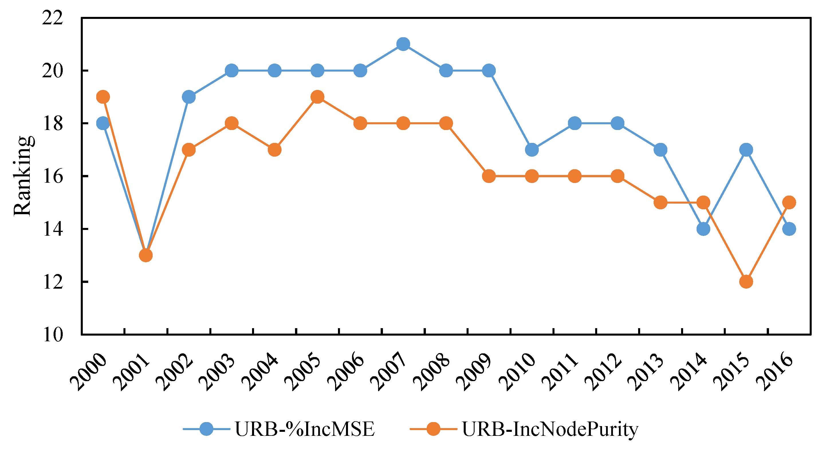
3.2. Interannual Variation Law of Influencing Factors

In order to research the annual change in the influencing factors of PM2.5 concentration, this paper analyzes the influence degree of the abovementioned influencing factors in different years and the results are shown in Figure A1. The performance evaluation results of the regression model in each year are shown in Table 3. In the annual research, the importance of natural factors in each year is generally higher than that of human factors. This may mean that natural factors are the main factors affecting PM2.5 concentration in the short term. Among all the human factors studied in this paper, only the factor of population density has the highest importance on PM2.5 concentration, which has remained within the top ten for a long time, and the degree of importance is increasing, having remained within the top five since 2011. This indicates that population density is the socio-economic factor with the highest impact on PM2.5 in the short term. During the study period, both GDP per capita and urban built-up area reached the top ten levels of importance in more than 30% of the time. Taking %Inc MSE as the evaluation standard, the top five influencing factors in 2000 were air pressure, temperature, elevation, wind speed and precipitation; the top five factors in 2016 were elevation, pressure, precipitation, temperature and population density. These indicate that the influences of human factors on PM2.5 concentration are strengthened.

3.3. Geographical Variation Patterns of Influencing Factors

In order to further clarify the geographical divergence patterns of the drivers of PM2.5 concentrations, this study analyzed the ranking of the %Inc MSE and Inc Node Purity of the influencing factors for 13 cities in the BTH, and drew heatmaps (Figure 4). In terms of the %Inc MSE values for each factor, the 13 cities are divided into three groups by geographical location (Figure 4a). The southeastern group includes Langfang, Handan, Xingtai, Cangzhou and Hengshui, for a total of five cities. The PM2.5 concentrations in these cities are mainly influenced by meteorology, topography, population and society, and the influence of natural factors is higher than that of human factors. The central group includes three cities, namely Beijing, Tianjin and Qinhuangdao. In these cities, human factors, including population, economy, land and society, have a greater influence on PM2.5 concentrations, while only one of the natural factors is more important, namely wind speed. This may be related to the high level of socio-economic development in these cities. The northwest group includes five cities, Zhangjiakou, Tangshan, Chengde, Shijiazhuang and Baoding. The driving factors in these cities are mainly meteorology, vegetation, population and economy, with meteorological factors having a slightly higher degree of influence than human factors. The ranking of the IncNodePurity values is essentially consistent with the %Inc MSE results (Figure 4b), with the only difference being that the southeastern group is reduced to three cities, Tangshan, Langfang and Cangzhou, while Handan and Xingtai are merged into the northwestern group. It is noteworthy that the central group remains in the same pattern and that the human factor continues to be overwhelmingly dominant.

4. Discussion

Air pollution has seriously affected human health and the sustainable development of social economy. PM2.5 is the primary pollutant in air pollution. In order to achieve the goal of reducing PM2.5 concentration, the primary task is to clarify the key influencing factors of PM2.5 concentration, and take corresponding measures to control these influencing factors, which can achieve the goal of reducing PM2.5 concentration.
Natural factors are the external factors affecting PM2.5 concentration (Figure 5). The results show that among the natural factors, sunshine hours, relative humidity, elevation, vegetation, wind speed, temperature and precipitation have the most significant impact on PM2.5 concentration in BTH. Moreover, the influence of these factors is higher than that of most human factors and plays an important role in the change in PM2.5 concentration. Similarly, Yang et al. [28] also concluded that the influence of natural factors is stronger than that of human factors in the comprehensive influencing factor analysis of PM2.5. However, Sun and Zhong [47] used principal component analysis to study 10 big cities in Beijing, Tianjin, Hebei, Yangtze River Delta, Pearl River Delta and other regions, and found that the sum of the two human factors of industrial activities and urban life contributed more than 70% to PM2.5 concentration, which are higher than the influence of three natural weather factors of temperature, humidity and precipitation on PM2.5 concentration. The main reason for this discrepancy may be that the entire area of the BTH also contains some counties with an average level of socio-economic development, and that natural factors such as elevation and wind speed, which have a large impact, have been added to this study. Adverse meteorological conditions will lead to the weakening of air convection and affect the diffusion of air pollutants, resulting in the increase in PM2.5 concentration. The fluctuation of terrain will block the transmission of pollutants between regions, thus affecting the local PM2.5 concentration. The close relationship between air pollution and vegetation has also been confirmed [48] in many studies. The effect of vegetation on the tissue absorption of particulate matter and the construction of a suitable environment for particulate matter deposition is obvious [49].
Human factors are the internal factors affecting PM2.5 concentration (Figure 5). Among the socio-economic factors selected in this paper, the urbanization rate, the total investment in fixed assets and the number of secondary industry employees have a significant impact on the PM2.5 concentration in Beijing, Tianjin and Hebei from 2000 to 2016, which means that human production and lifestyle are important factors affecting the PM2.5 concentration in BTH. However, from the analysis of influencing factors of PM2.5 concentration in a single year, it is found that population density is the most important socio-economic factor affecting PM2.5 concentration for many years and population agglomeration has a significant impact on local PM2.5 concentration.
Different from the results of the multi-year comprehensive analysis, population density, GDP per capita and urban built-up area have a more significant impact on PM2.5 in the single year study. The finding that the urbanization rate has no significant impact on PM2.5 is consistent with the previous research results of some single years [50]. This shows that the urbanization rate may not be the main indicator to predict PM2.5 concentration in the short term and its impact on PM2.5 concentration may have a time lag effect. In addition, the importance ranking of the influencing factor of urbanization rate has increased significantly after 2012 (Figure 6) from the annual change trend of the importance ranking of the impact degree of urbanization rate. In other words, the impact of urbanization rate on PM2.5 has been strengthened in recent years. Statistics show that the urbanization rate of BTH increased from 58.93% to 63.88% with an average annual increase of 1.24 percentage points from 2012 to 2016. Compared with 2000–2012, the urbanization rate during this period was higher, but the growth rate was lower (0.42 percentage points lower). This shows that when analyzing the influencing factors of PM2.5 under the development background of relatively high urbanization rate, it is more necessary to consider the urbanization rate, which represents the level of population urbanization.
In the indicator system of influencing factors constructed in this paper, the influence of natural factors such as terrain, vegetation and climate on PM2.5 concentration can be proved, which is helpful to analyze the influence mechanism of these natural factors on PM2.5 concentration, such as low wind speed and high altitude affecting the diffusion of pollutants. However, due to the limitation of data, the analysis in this paper could only conclude that among the urbanization factors, human production, living activities, and land-use patterns affect PM2.5 concentration, which makes it difficult to determine the source of pollutants that lead to the increase in PM2.5 concentration. In other words, which of the factors, including domestic heating and cooking, car exhaust emissions and industrial exhaust emissions, has a greater impact on PM2.5 pollution is difficult to analyze in this paper, and this direction needs further research in the future.

5. Conclusions

On the basis of the macro background of urbanization with Chinese characteristics and facing the practical problems of serious PM2.5 pollution in BTH, this paper attempts to construct the comprehensive influencing factor analysis indicator system of PM2.5 in BTH from the natural factors of meteorology, terrain, vegetation, etc., and human factors of population urbanization, land urbanization, economic urbanization, and social urbanization, among others. Then, it uses the random forest model to analyze the influencing factors of PM2.5 in BTH from 2000 to 2016, as well as some discussions about the interannual variation law of the main influencing factors. The main conclusions are as follows:
(1)
PM2.5 pollution is a comprehensive problem involving the intersection of nature and society. Among them, natural factors such as sunshine hours, relative humidity, elevation, vegetation, wind speed, average temperature, precipitation, temperature daily range and air pressure, as well as socio-economic factors such as urbanization rate, total investment in fixed assets and the number of secondary industry employees, are the main factors affecting PM2.5 concentration. In contrast, factors such as population density, GDP, the proportion of added value of secondary industry in GDP, per capita GDP and total population have relatively little impact on PM2.5 concentration.
(2)
There is a nonlinear relationship between PM2.5 concentration and influencing factors. With the increase in sunshine hours and wind speed, PM2.5 concentration remains stable at first, then decreases sharply and returns to stability; with the increase in relative humidity, vegetation index, average temperature, air pressure, urbanization rate and total investment in fixed assets, PM2.5 concentration stabilizes at first, then rises sharply and returns to stability; with the increase in elevation, it shows a fluctuating downward trend; with the increase in temperature daily range, it shows a trend of rising up first and then decreasing; in addition, its change is less obvious with the increase in precipitation and the number of secondary industry employees.
(3)
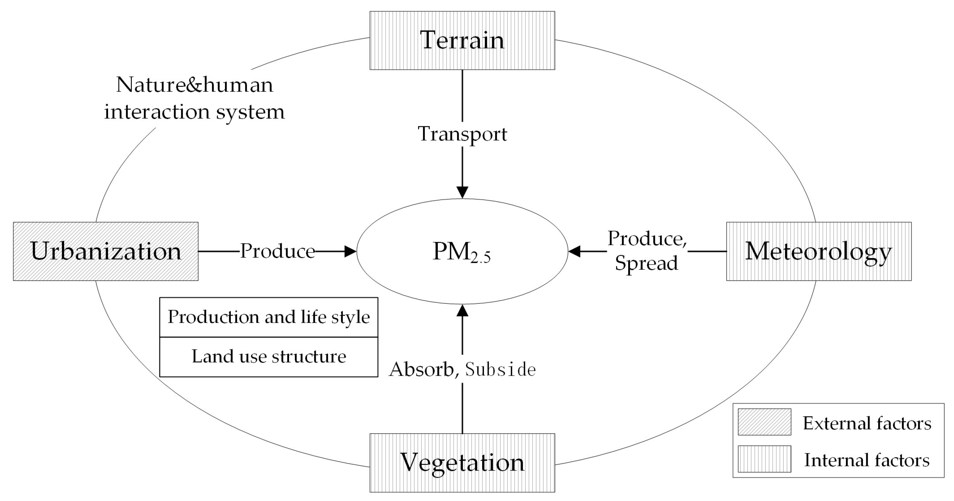
Compared with urbanization factors, the terrain, climate, vegetation and other natural factors account for a higher proportion of the main influencing factors of PM2.5 concentration. They are the main factors affecting PM2.5 concentration in BTH and affect the generation, diffusion and settlement of PM2.5. However, the influence of some urbanization factors has been strengthened in recent years. Urbanization, reflecting human production and living activities, is the cause of PM2.5 carrying harmful substances and is also the key factor affecting human health. Moreover, the natural background elements are difficult to be changed through human intervention in the short term. Starting with human factors, the adjustment and control of PM2.5 pollution sources will become a powerful way to improve the current situation of PM2.5 pollution.

Author Contributions

Conceptualization, S.G. and X.T.; methodology, S.G.; software, S.G.; validation, S.G. and X.T.; formal analysis, S.G.; resources, X.T. and L.L.; data curation, S.G.; writing—original draft preparation, S.G.; writing—review and editing, X.T. and L.L.; visualization, S.G.; supervision, X.T.; project administration, X.T. and L.L.; funding acquisition, X.T. All authors have read and agreed to the published version of the manuscript.

Funding

This research was funded by the Strategic Priority Research Program of the Chinese Academy of Sciences (Grant XDA23100301) and the BJAST Budding Talent Program(Grant BGS201907).

Institutional Review Board Statement

Not applicable.

Informed Consent Statement

Not applicable.

Data Availability Statement

Publicly available datasets were analyzed in this study. These data can be found here: https://sedac.ciesin.columbia.edu/ (accessed on 4 June 2020), http://data.cma.cn/ (accessed on 5 June 2020), https://www.resdc.cn/ (accessed on 1 June 2020), and http://maps.elie.ucl.ac.be/CCI/viewer/ (accessed on 16 June 2020).

Conflicts of Interest

The authors declare no conflict of interest.

Appendix A

Figure A1. Ranking of importance factors of PM2.5 concentrations in BTH, 2000–2016. (a) 2000; (b) 2001; (c) 2002; (d) 2003; (e) 2004; (f) 2005; (g) 2006; (h) 2007; (i) 2008; (j) 2009; (k) 2010; (l) 2011; (m) 2012; (n) 2013; (o) 2014; (p) 2015; (q) 2016. Each variable name is the same as in Figure 2.
Atmosphere 14 00381 g0a1

References

  1. Chen, M.; Gong, Y.; Lu, D.; Ye, C. Build a people-oriented urbanization: China’s new-type urbanization dream and Anhui model. Land Use Policy 2019, 80, 1–9. [Google Scholar] [CrossRef]
  2. Chen, M.; Liu, W.; Lu, D. Challenges and the way forward in China’s new-type urbanization. Land Use Policy 2016, 55, 334–339. [Google Scholar] [CrossRef]
  3. Wang, Z.; Liang, L.; Wang, X. Spatiotemporal evolution of PM2.5 concentrations in urban agglomerations of China. J. Geogr. Sci. 2021, 31, 878–898. [Google Scholar] [CrossRef]
  4. Wang, Z.-B.; Fang, C.-L. Spatial-temporal characteristics and determinants of PM2.5 in the Bohai Rim Urban Agglomeration. Chemosphere 2016, 148, 148–162. [Google Scholar] [CrossRef] [PubMed]
  5. Wang, J.; Li, T.; Li, Z.; Fang, C. Study on the Spatial and Temporal Distribution Characteristics and Influencing Factors of Particulate Matter Pollution in Coal Production Cities in China. Int. J. Environ. Res. Public Health 2022, 19, 3228. [Google Scholar] [CrossRef]
  6. Gryech, I.; Ghogho, M.; Mahraoui, C.; Kobbane, A. An Exploration of Features Impacting Respiratory Diseases in Urban Areas. Int. J. Environ. Res. Public Health 2022, 19, 3095. [Google Scholar] [CrossRef]
  7. Li, L.; Lei, Y.; Wu, S.; Chen, J.; Yan, D. The health economic loss of fine particulate matter (PM2.5) in Beijing. J. Clean. Prod. 2017, 161, 1153–1161. [Google Scholar] [CrossRef]
  8. Hu, J.; Wang, Y.; Ying, Q.; Zhang, H. Spatial and temporal variability of PM2.5 and PM10 over the North China Plain and the Yangtze River Delta, China. Atmos. Environ. 2014, 95, 598–609. [Google Scholar] [CrossRef]
  9. Yang, S.; Ma, Y.L.; Duan, F.K.; He, K.B.; Wang, L.T.; Wei, Z.; Zhu, L.D.; Ma, T.; Li, H.; Ye, S.Q. Characteristics and formation of typical winter haze in Handan, one of the most polluted cities in China. Sci. Total Environ. 2018, 613–614, 1367–1375. [Google Scholar] [CrossRef]
  10. Li, X.; Ma, Y.; Wang, Y.; Liu, N.; Hong, Y. Temporal and spatial analyses of particulate matter (PM10 and PM2.5) and its relationship with meteorological parameters over an urban city in northeast China. Atmos. Res. 2017, 198, 185–193. [Google Scholar] [CrossRef]
  11. Zhang, S.; Han, L.; Zhou, W.; Li, W. Impact of urban population on concentrations of nitrogen dioxide (NO2) and fine particles (PM2.5) in China. Acta Ecol. Sin. 2016, 36, 5049–5057. [Google Scholar]
  12. Duo, B.; Cui, L.; Wang, Z.; Li, R.; Zhang, L.; Fu, H.; Chen, J.; Zhang, H.; Qiong, A. Observations of atmospheric pollutants at Lhasa during 2014–2015: Pollution status and the influence of meteorological factors. J. Environ. Sci. 2018, 63, 28–42. [Google Scholar] [CrossRef] [PubMed]
  13. Hasheminassab, S.; Daher, N.; Ostro, B.D.; Sioutas, C. Long-term source apportionment of ambient fine particulate matter (PM2.5) in the Los Angeles Basin: A focus on emissions reduction from vehicular sources. Environ. Pollut. 2014, 193, 54–64. [Google Scholar] [CrossRef] [PubMed]
  14. Tunno, B.J.; Dalton, R.; Michanowicz, D.R.; Shmool, J.L.C.; Kinnee, E.; Tripathy, S.; Cambal, L.; Clougherty, J.E. Spatial patterning in PM2.5 constituents under an inversion-focused sampling design across an urban area of complex terrain. J. Expo. Sci. Environ. Epidemiol. 2016, 26, 385–396. [Google Scholar] [CrossRef] [PubMed] [Green Version]
  15. Karagulian, F.; Belis, C.A.; Dora, C.F.C.; Prüss-Ustün, A.M.; Bonjour, S.; Adair-Rohani, H.; Amann, M. Contributions to cities’ ambient particulate matter (PM): A systematic review of local source contributions at global level. Atmos. Environ. 2015, 120, 475–483. [Google Scholar] [CrossRef]
  16. Zhao, Y.-B.; Gao, P.-P.; Yang, W.-D.; Ni, H.-G. Vehicle exhaust: An overstated cause of haze in China. Sci. Total Environ. 2018, 612, 490–491. [Google Scholar] [CrossRef]
  17. Zhou, C.; Chen, J.; Wang, S. Examining the effects of socioeconomic development on fine particulate matter (PM2.5) in China’s cities using spatial regression and the geographical detector technique. Sci. Total Environ. 2018, 619–620, 436–445. [Google Scholar] [CrossRef]
  18. Gao, J.; Tian, H.; Cheng, K.; Lu, L.; Zheng, M.; Wang, S.; Hao, J.; Wang, K.; Hua, S.; Zhu, C.; et al. The variation of chemical characteristics of PM2.5 and PM10 and formation causes during two haze pollution events in urban Beijing, China. Atmos. Environ. 2015, 107, 1–8. [Google Scholar] [CrossRef]
  19. Lanzaco, B.L.; Olcese, L.E.; Querol, X.; Toselli, B.M. Analysis of PM2.5 in Córdoba, Argentina under the effects of the El Niño Southern Oscillation. Atmos. Environ. 2017, 171, 49–58. [Google Scholar] [CrossRef]
  20. Cesari, D.; Donateo, A.; Conte, M.; Merico, E.; Giangreco, A.; Giangreco, F.; Contini, D. An inter-comparison of PM2.5 at urban and urban background sites: Chemical characterization and source apportionment. Atmos. Res. 2016, 174–175, 106–119. [Google Scholar] [CrossRef]
  21. Masiol, M.; Hopke, P.K.; Felton, H.D.; Frank, B.P.; Rattigan, O.V.; Wurth, M.J.; LaDuke, G.H. Source apportionment of PM2.5 chemically speciated mass and particle number concentrations in New York City. Atmos. Environ. 2017, 148, 215–229. [Google Scholar] [CrossRef]
  22. Saraga, D.E.; Tolis, E.I.; Maggos, T.; Vasilakos, C.; Bartzis, J.G. PM2.5 source apportionment for the port city of Thessaloniki, Greece. Sci. Total Environ. 2019, 650, 2337–2354. [Google Scholar] [CrossRef]
  23. Chen, J.; Zhou, C.; Wang, S.; Li, S. Impacts of energy consumption structure, energy intensity, economic growth, urbanization on PM2.5 concentrations in countries globally. Appl. Energy 2018, 230, 94–105. [Google Scholar] [CrossRef]
  24. Lu, D.; Xu, J.; Yang, D.; Zhao, J. Spatio-temporal variation and influence factors of PM2.5 concentrations in China from 1998 to 2014. Atmos. Pollut. Res. 2017, 8, 1151–1159. [Google Scholar] [CrossRef]
  25. Wang, N.; Zhu, H.; Guo, Y.; Peng, C. The heterogeneous effect of democracy, political globalization, and urbanization on PM2.5 concentrations in G20 countries: Evidence from panel quantile regression. J. Clean. Prod. 2018, 194, 54–68. [Google Scholar] [CrossRef]
  26. Lin, G.; Fu, J.; Jiang, D.; Hu, W.; Dong, D.; Huang, Y.; Zhao, M. Spatio-temporal variation of PM2.5 concentrations and their relationship with geographic and socioeconomic factors in China. Int. J. Environ. Res. Public Health 2013, 11, 173–186. [Google Scholar] [CrossRef] [Green Version]
  27. Luo, J.; Du, P.; Samat, A.; Xia, J.; Che, M.; Xue, Z. Spatiotemporal Pattern of PM2.5 Concentrations in Mainland China and Analysis of Its Influencing Factors using Geographically Weighted Regression. Sci. Rep. 2017, 7, 40607. [Google Scholar] [CrossRef] [Green Version]
  28. Yang, D.; Wang, X.; Xu, J.; Xu, C.; Lu, D.; Ye, C.; Wang, Z.; Bai, L. Quantifying the influence of natural and socioeconomic factors and their interactive impact on PM2.5 pollution in China. Environ. Pollut. 2018, 241, 475–483. [Google Scholar] [CrossRef]
  29. Hua, Y.; Cheng, Z.; Wang, S.; Jiang, J.; Chen, D.; Cai, S.; Fu, X.; Fu, Q.; Chen, C.; Xu, B.; et al. Characteristics and source apportionment of PM2.5 during a fall heavy haze episode in the Yangtze River Delta of China. Atmos. Environ. 2015, 123, 380–391. [Google Scholar] [CrossRef]
  30. Jiang, T.; Chen, B.; Nie, Z.; Ren, Z.; Tang, S. Estimation of hourly full-coverage PM2.5 concentrations at 1-km resolution in China using a two-stage random forest model. Atmos. Res. 2020, 248, 105146. [Google Scholar] [CrossRef]
  31. Zamani, M. PM2.5 Prediction Based on Random Forest, XGBoost, and Deep Learning Using Multisource Remote Sensing Data. Atmosphere 2019, 10, 373. [Google Scholar] [CrossRef]
  32. Tza, B.; Wh, A.; Hui, Z.; Yc, A.; Hsa, B.; Sfa, B. Satellite-based ground PM 2.5 estimation using a gradient boosting decision tree. Chemosphere 2021, 268, 128801. [Google Scholar]
  33. Dai, H.; Huang, G.; Zeng, H.; Zhou, F. PM2.5 volatility prediction by XGBoost-MLP based on GARCH models. J. Clean. Prod. 2022, 356, 131898. [Google Scholar] [CrossRef]
  34. Dai, H.; Huang, G.; Zeng, H.; Yu, R. Haze Risk Assessment Based on Improved PCA-MEE and ISPO-LightGBM Model. Systems 2022, 10, 263. [Google Scholar] [CrossRef]
  35. Parkhurst, D.F.; Brenner, K.P.; Dufour, A.P.; Wymer, L.J. Indicator bacteria at five swimming beaches-analysis using random forests. Water Res. 2005, 39, 1354–1360. [Google Scholar] [CrossRef]
  36. Grekousis, G.; Feng, Z.; Marakakis, I.; Lu, Y.; Wang, R. Ranking the importance of demographic, socioeconomic, and underlying health factors on US COVID-19 deaths: A geographical random forest approach. Health Place 2022, 74, 102744. [Google Scholar] [CrossRef]
  37. Xue, F.; Yao, E. Adopting a random forest approach to model household residential relocation behavior. Cities 2022, 125, 103625. [Google Scholar] [CrossRef]
  38. Zhou, W.; Yang, H.; Xie, L.; Li, H.; Huang, L.; Zhao, Y.; Yue, T. Hyperspectral inversion of soil heavy metals in Three-River Source Region based on random forest model. Catena 2021, 202, 105222. [Google Scholar] [CrossRef]
  39. Wu, H.; Lin, A.; Xing, X.; Song, D.; Li, Y. Identifying core driving factors of urban land use change from global land cover products and POI data using the random forest method. Int. J. Appl. Earth Obs. Geoinf. 2021, 103, 102475. [Google Scholar] [CrossRef]
  40. Lu, D. Function orientation and coordinating development of subregions within the Jing-Jin-Ji Urban Agglomeration. Prog. Geogr. 2015, 34, 265–270. [Google Scholar] [CrossRef]
  41. Chen, M.; Guo, S.; Hu, M.; Zhang, X. The spatiotemporal evolution of population exposure to PM2.5 within the Beijing-Tianjin-Hebei urban agglomeration, China. J. Clean. Prod. 2020, 265, 121708. [Google Scholar] [CrossRef]
  42. van Donkelaar, A.; Martin, R.V.; Brauer, M.; Hsu, N.C.; Kahn, R.A.; Levy, R.C.; Lyapustin, A.; Sayer, A.M.; Winker, D.M. Global Estimates of Fine Particulate Matter using a Combined Geophysical-Statistical Method with Information from Satellites, Models, and Monitors. Environ. Sci. Technol. 2016, 50, 3762–3772. [Google Scholar] [CrossRef]
  43. Chen, M.; Liu, W.; Lu, D.; Chen, H.; Ye, C. Progress of China’s new-type urbanization construction since 2014: A preliminary assessment. Cities 2018, 78, 180–193. [Google Scholar] [CrossRef]
  44. Zhou, Y.; Chen, M.; Tang, Z.; Mei, Z. Urbanization, land use change, and carbon emissions: Quantitative assessments for city-level carbon emissions in Beijing-Tianjin-Hebei region. Sustain. Cities Soc. 2021, 66, 102701. [Google Scholar] [CrossRef]
  45. Chen, M.; Sui, Y.; Liu, W.; Liu, H.; Huang, Y. Urbanization patterns and poverty reduction: A new perspective to explore the countries along the Belt and Road. Habitat Int. 2019, 84, 1–14. [Google Scholar] [CrossRef]
  46. Breiman, L. Random Forests. Mach. Learn. 2001, 45, 5–32. [Google Scholar] [CrossRef] [Green Version]
  47. Sun, J.; Zhong, Y. Economic Analysis on the Factors Influencing PM2.5 in China’s Metropolises: An Empirical Study Based on City-Level Panel Data. Ecol. Econ. 2015, 31, 5. [Google Scholar]
  48. Somvanshi, S.S.; Kumari, M. Comparative analysis of different vegetation indices with respect to atmospheric particulate pollution using sentinel data. Appl. Comput. Geosci. 2020, 7, 100032. [Google Scholar] [CrossRef]
  49. Diener, A.; Mudu, P. How can vegetation protect us from air pollution? A critical review on green spaces’ mitigation abilities for air-borne particles from a public health perspective-with implications for urban planning. Sci. Total Environ. 2021, 796, 148605. [Google Scholar] [CrossRef]
  50. Zhan, D.; Kwan, M.-P.; Zhang, W.; Yu, X.; Meng, B.; Liu, Q. The driving factors of air quality index in China. J. Clean. Prod. 2018, 197, 1342–1351. [Google Scholar] [CrossRef]
Figure 1. Distribution of natural elements in the Beijing–Tianjin–Hebei urban agglomeration (BTH) (taking 2016 as an example).
Atmosphere 14 00381 g001
Figure 2. Priority ranking of factors affecting PM2.5 concentrations in the BTH from 2000 to 2016. (a) Ranking of %Inc MSE; (b) Ranking of Inc Node Purity. Each variable name is the same as in Table 1.
Atmosphere 14 00381 g002
Figure 3. Partial dependency plots of factors affecting PM2.5 concentrations in the BTH from 2000 to 2016. (a) SSH; (b) RHU; (c) ELE; (d) NDVI; (e) WIN; (f) TEM; (g) TEMR; (h) PRE; (i) PRS; (j) URB; (k) INV; (l) INDU. Each variable name is the same as in Table 1.
Atmosphere 14 00381 g003
Figure 4. Heatmaps of factors affecting PM2.5 concentrations in the BTH. (a) Ranking of %Inc MSE; (b) Ranking of Inc Node Purity. Each variable name is the same as in Table 1.
Atmosphere 14 00381 g004
Figure 5. Effect of PM2.5 concentration.
Atmosphere 14 00381 g005
Figure 6. Rank change in importance of influence of urbanization rate on PM2.5 concentration. URB refers to urbanization.
Atmosphere 14 00381 g006
Table 1. PM2.5 impact factor indicator system.
CategoryNameSymbolUnitDescriptionData SourcesSpatial InformationTemporal Information
Natural factorsMeteorologyTemperatureTEM°CAnnual average temperaturedata.cma.cn (accessed on 5 June 2020)174 stations in BTH2010–2016
Temperature daily rangeTEMR°CAnnual average daily temperature range
Sunshine hoursSSHhAnnual average sunshine hours
PrecipitationPREmmAnnual precipitation
Relative humidityRHU%Average relative humidity
Wind speedWINm/sAverage wind speed
PressurePRShPaMean air pressure
TerrainElevationELEmMean elevationwww.resdc.cn (accessed on 1 June 2020)1 km2010–2016
VegetationNDVINDVI-Normalized Difference Vegetation Indexwww.resdc.cn (accessed on 1 June 2020)1 km2010–2016
Human factorsPopulation urbanizationPopulationPOPpeopleTotal resident population at the end of the yearwww.stats.gov.cn (accessed on 10 June 2020), tjj.beijing.gov.cn (accessed on 10 June 2020), stats.tj.gov.cn (accessed on 10 June 2020), www.hetj.gov.cn (accessed on 10 June 2020)County scale2010–2016
Population densityDENpeople/m2Population density per unit area
Urbanization rateURB%Percentage of urban permanent population to total permanent population
Economic urbanizationGDPGDPCNYGross Domestic Productwww.stats.gov.cn (accessed on 10 June 2020), tjj.beijing.gov.cn (accessed on 10 June 2020), stats.tj.gov.cn (accessed on 10 June 2020), www.hetj.gov.cn (accessed on 10 June 2020) County scale2010–2016
Per capita GDPPGDPCNY/personPer capita GDP
Proportion of secondary industryIND%The proportion of added value of secondary industry in GDP
Gross industrial output valueGIOCNYGross industrial output value above designated size
Land urbanizationUrban built-up areaBUIkm2Urban areamaps.elie.ucl.ac.be/CCI/viewer/ (accessed on 16 June 2020)300 m2010–2016
Road mileageROAkmAll road mileagewww.stats.gov.cn (accessed on 10 June 2020), tjj.beijing.gov.cn (accessed on 10 June 2020), stats.tj.gov.cn (accessed on 10 June 2020), www.hetj.gov.cn (accessed on 10 June 2020)County scale
Social urbanizationEmployees in the secondary industryINDUpeopleNumber of employees in the secondary industrywww.stats.gov.cn (accessed on 10 June 2020), tjj.beijing.gov.cn (accessed on 10 June 2020), stats.tj.gov.cn (accessed on 10 June 2020), www.hetj.gov.cn (accessed on 10 June 2020) County scale2010–2016
Total retail sales of consumer goodsCONCNYTotal retail sales of consumer goods
Total investment in fixed assetsINVCNYTotal investment in fixed assets
Table 2. Number of influence factor variables and root mean squared error (MSE).
Number of VariablesMSENumber of VariablesMSENumber of VariablesMSENumber of VariablesMSE
10.0182970.01124130.01054190.01045
20.0141180.01109140.01054200.01041
30.0128690.01094150.01055210.01054
40.01214100.01078160.01042
50.01176110.01067170.01039
60.01144120.01057180.01043
Table 3. Performance evaluation of random forest regression models from 2000 to 2016.
Year200020012002200320042005200620072008
Mean of squared residuals0.01240.01390.01270.00680.00720.00780.00710.00500.0062
% Var explained96.6193.7495.1596.1896.9396.4596.9997.7197.01
Year20092010201120122013201420152016
Mean of squared residuals0.00510.00450.00580.00530.00490.00970.00510.0061
% Var explained97.4197.7996.8897.2797.6495.5997.3397.40
Disclaimer/Publisher’s Note: The statements, opinions and data contained in all publications are solely those of the individual author(s) and contributor(s) and not of MDPI and/or the editor(s). MDPI and/or the editor(s) disclaim responsibility for any injury to people or property resulting from any ideas, methods, instructions or products referred to in the content.

