Article

CMIP6 GCM Validation Based on ECS and TCR Ranking for 21st Century Temperature Projections and Risk Assessment

Department of Earth Sciences, Environment and Georesources, University of Naples Federico II, Complesso Universitario di Monte S. Angelo, Via Cinthia, 21, 80126 Naples, Italy
Atmosphere 2023, 14(2), 345; https://doi.org/10.3390/atmos14020345
Submission received: 31 December 2022 / Revised: 3 February 2023 / Accepted: 7 February 2023 / Published: 9 February 2023
(This article belongs to the Section Climatology)

Abstract

:
Global climate models (GCMs) from the sixth Coupled Model Intercomparison Project Phases (CMIP6) have been employed to simulate the twenty-first-century temperatures for the risk assessment of future climate change. However, their transient climate response (TCR) ranges from 1.2 to 2.8 °C, whereas their equilibrium climate sensitivity (ECS) ranges from 1.8 to 5.7 °C, leading to large variations in the climatic impact of an anthropogenic increase in atmospheric CO2 levels. Moreover, there is growing evidence that many GCMs are running “too hot” and are hence unreliable for directing policies for future climate changes. Here, I rank 41 CMIP6 GCMs according to how successfully they hindcast the global surface warming between 1980 and 2021 using both their published ECS and TCR estimates. The sub-ensemble of GCMs with the best performance appears to be composed of the models with ECS ranging between 1.8 and 3.0 °C (which confirms previous studies) and TCR ranging between 1.2 and 1.8 °C. This GCM sub-ensemble is made up of a total of 17 models. Depending on the emission scenarios, these GCMs predict a 2045–2055 warming of 1.5–2.5 °C compared to the pre-industrial era (1850–1900). As a result, the global aggregated impact and risk estimates seem to be moderate, which implies that any negative effects of future climate change may be adequately addressed by adaptation programs. However, there are also doubts regarding the actual magnitude of global warming, which might be exaggerated because of urban heat contamination and other local non-climatic biases. A final section is dedicated to highlighting the divergences observed between the global surface temperature records and a number of alternative temperature reconstructions from lower troposphere satellite measurements, tree-ring-width chronologies, and surface temperature records based on rural stations alone. If the global warming reported by the climate records is overestimated, the real ECS and TCR may be significantly lower than what is produced by the CMIP6 GCMs, as some independent studies have already suggested, which would invalidate all of the CMIP6 GCMs.

Graphical Abstract

1. Introduction

Potential future climate change, societal development, and climate adaptation and/or mitigation efforts are all considered in the risk assessment of future climate change [1]. Climate change during the twenty-first century has been evaluated using global climate model (GCM) simulations from the fifth and sixth Coupled Model Intercomparison Projects (CMIP5, CMIP6) of the World Climate Research Programme [2,3]. The models employ a standard set of unique historical forcing functions from 1850 to 2014. The emissions from hypothetical Representative Concentration Pathways (RCPs) and Shared Socioeconomic Pathways (SSPs) scenarios are used to determine forecasts from 2015 to 2100. These span a wide range of potential outcomes that might affect how vulnerable people are to and exposed to climate change in the future. The near-term (2021–2040), mid-term (2041–2060), and long-term (2081–2100) prospective reference periods are typically used to evaluate the consequences and dangers of climate change. The pre-industrial global surface temperature is most closely represented by the reference period between 1850 and 1900.
More than 50 CMIP6 GCMs are available [4]. Despite utilizing identical radiative forcing functions, their predictions for the twenty-first century differ greatly from one another. The fundamental issue is that a significant percentage of GCMs seem to be operating “too hot” [5,6,7,8,9,10,11,12,13,14,15,16,17,18], which suggests that climate change policy should disregard the projections from the “hot” models.
For instance, the CMIP6 GCMs evaluate that doubling atmospheric CO2 concentrations from pre-industrial levels (from 280 to 560 ppm) will result in a global surface warming that could span from 1.8 to 5.7 °C. However, the ECS values larger than 5 °C already surpassed those of the CMIP5 GCMs [2]. In fact, throughout the preceding 40 years, various climate models have consistently maintained an ECS range of 1.5 °C–4.5 °C.
Climate scientists are uncertain of how strong the climate’s response to greenhouse gases may be. A major dilemma is which GCMs should be utilized for climate change policy for future decades. A reasonable choice could be to utilize those models that better hindcast the global warming of the past decades. The assessment of a suitable range of climate sensitivity, which should be based on actual experimental data, is, therefore, a hot issue of discussion right now [5].
For example, by combining a number of evidence from palaeoclimate, surface temperatures, ocean heat content, and modeling, Sherwood et al. [19] concluded that the ECS is likely (with a 66% chance) in the range of 2.6–3.9 ° C, and very likely (with a 90% chance) between 2.3 and 4.7 °C. The IPCC [1] and Hausfather et al. [5] accepted these estimates and excluded the projections made by the too-hot models, which account for about one-third of all CMIP6 GCMs. However, Lewis [17] reanalyzed the same data and, from multiple lines of evidences concluded that the actual ECS median should be 2.16 °C, its 17–83% range is 1.75–2.7 ° C, and its 5–95% range is 1.55–3.2 ° C. Scafetta [12,18] also reached a similar conclusion using a methodology that will be extended in the present paper. Lewis [17] and Scafetta [12,18] would imply that about two-thirds of the CMIP6 GCMs should be screened out for the policy. Finally, McKitrick and Christy [7] compared the tropospheric temperature records against the CMIP6 GCMs’ hindcasts and concluded that all CMIP6 GCMs are running too hot. The latter finding would require a new generation of GCMs with lower ECS values than the CMIP6 ones. This ambiguity needs to be clarified.
Additionally, it should be noted that there are several definitions of climate sensitivity. For instance, Hausfather et al. [5] proposed the selection of suitable GCMs using not their ECS but their transient climate response (TCR). By accepting the analysis by Sherwood et al. [19] and the choices of the IPCC [1], they proposed to exclude the models with TCR beyond their estimated “probable” (66% probability range) range of 1.4–2.2 ° C. Here, I will re-assess this range as well.
The equilibrium climate sensitivity (ECS) is the long-term temperature rise (equilibrium global mean near-surface air temperature) that is expected to result from a doubling of the atmospheric CO2 concentration [3]. Once the CO2 concentration has stopped rising, and the majority of the feedback has had time to fully take effect, the new global mean near-surface air temperature is predicted. However, after CO2 has doubled, it can take centuries or even millennia to reach a new equilibrium temperature. According to the IPCC Sixth Assessment Report (AR6) [3], there would be a high degree of confidence that ECS is between 2.5 and 4 °C, with a best estimate of 3 ° C, although the CMIP6 GCMs predict that the ECS could be between 1.8 and 5.7 ° C.
The transient climate response (TCR) is defined as the change in the global mean surface temperature, averaged over a 20-year period, centered at the time of atmospheric carbon dioxide doubling, in a climate model simulation in which the atmospheric CO2 concentration increases at 1% per year [3]. TCR is calculated using simulations with shorter time periods. Because slower feedbacks, which amplify the temperature increase, take longer to fully react to an increase in atmospheric CO2 concentration, the transient response is smaller than the equilibrium climate sensitivity. For instance, after a perturbation, the deep ocean takes several centuries to achieve a new steady state while continuing to cool the top ocean as a heatsink. The CMIP6 GCMs predict that the TCR could be between 1.2 and 2.8 ° C.
Because of the quick buffering effects of the oceans, ECS is larger than TCR. In order to simulate the complete time period during which strong feedbacks, such as fully equilibrating ocean temperatures, continue to influence global temperatures in the model, the ECS is calculated using computer models that run for a duration of centuries. There are methods, nevertheless, that use less processing power.
Scafetta [12,18] and Lewis [17] reevaluated the equilibrium climate sensitivity (ECS) problem utilizing information from a variety of sources. These authors reached a similar conclusion: the actual ECS should be between 1.5 and 3.0 ° C. This finding is important for policymakers because it suggests that the predicted risk of climate change will be moderate in the next decades and that adaptation strategies will be sufficient to address any negative effects. In fact, the low-ECS GCMs are those that project the least warming for the twenty-first century.
However, ECS could be a less relevant indicator than TCR for choosing climate change policy because of the extensive time scales needed for the climate system to reach a new equilibrium. Here, I add to the work performed by Scafetta [11,12,18] by rating the CMIP6 GCMs in accordance with both their ECS and TCR values reported in the literature [3,5]. The risk level of climate change is then assessed using the ECS and TCR GCM sub-ensembles that appear to better hindcast the warming from 1980 to 2021.
Finally, Section 4 touches on some unresolved issues concerning the magnitude of the global surface warming as reported by the official global surface temperature records, and the potential necessity of disregarding all of the CMIP6 GCMs when formulating climate change policies for the twenty-first century.

2. Data and Methods

The following monthly near-surface air temperature records are used: ERA5-T2m [20,21]; HadCRUT5 [22]; GISTEMP v4 [23]; NOAAGlobalTemp v5 [24]; Japanese Meteorological Agency (JMA) [25]; the Berkeley Earth (BE) group [26]. These surface temperature records suggest that the global surface warming Δ T m e a n from 1980–1990 to 2011–2021 could have varied from 0.52 to 0.59 ° C [12].
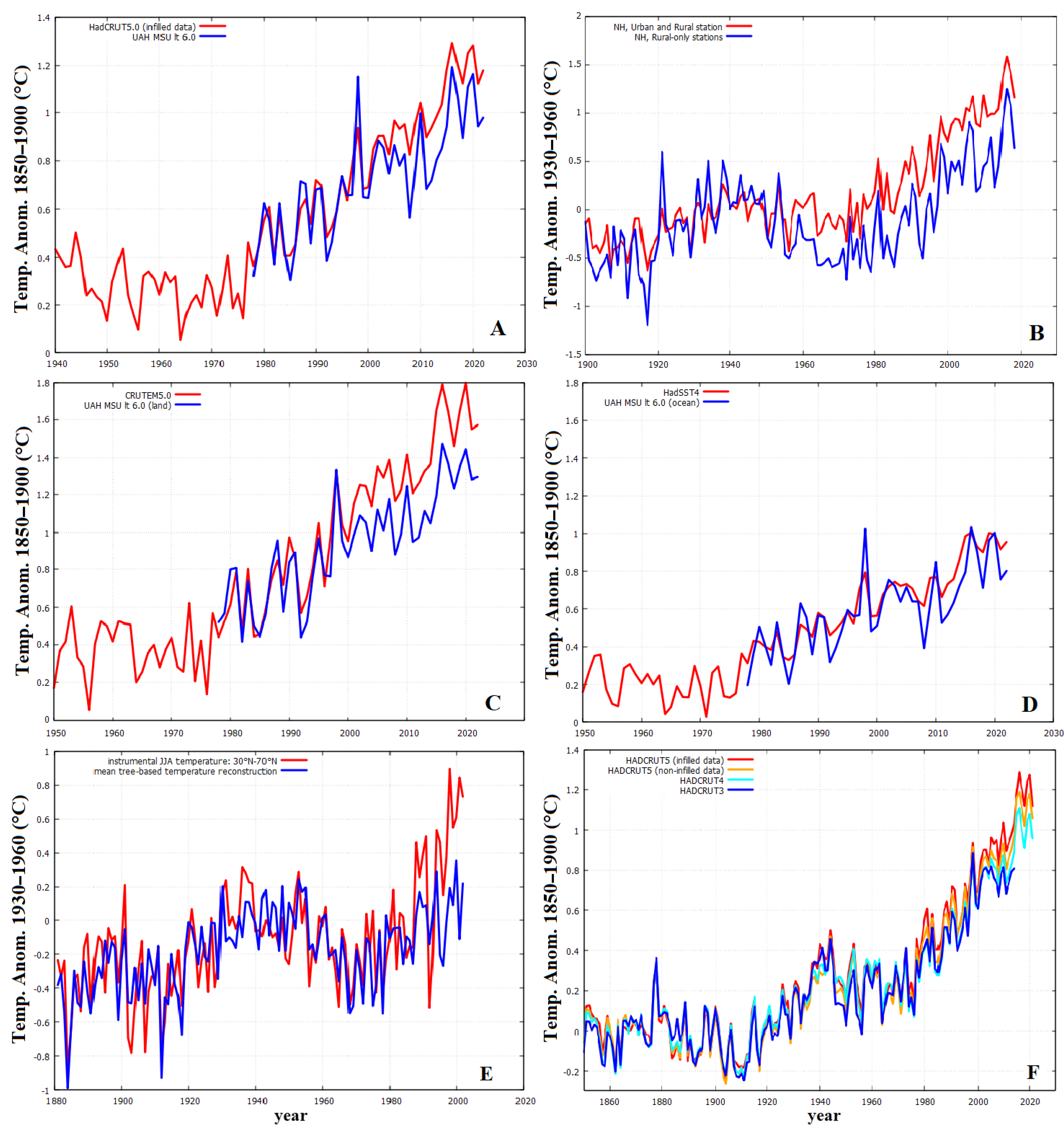
Section 4 compares the above temperature records with other records to discuss the likelihood that the global surface temperature records might be warm biased [27,28]. To highlight this issue, the following figures show the 0.52–0.59 ° C range of the warming reported by the global surface temperature records together with the 0.40 ° C warming reported by the lower troposphere UAH-MSU-lt v6 record [29] during the same period.
Out of all the temperature records that are currently available, the UAH-MSU-lt satellite record is explicitly used in this case mainly because it is the one that demonstrates the least rising trend and may be taken as the lowest limit provided by the scientific literature for the actual warming that has occurred at the surface. The apparent paradox of comparing a lower troposphere satellite-based temperature record to observations or model simulations at the surface is resolved by taking into consideration that the GCMs indicate that the troposphere warming should be larger than at the surface [6,7,8], and that our initial assumption is that the GCMs’ assertion that greenhouse gases are the primary cause of global warming may be true. Therefore, the warming shown by the UAH-MSU-lt satellite record should theoretically be even larger than that at the surface: see also the discussion in Scafetta [12] and the discussion in Section 4.
The time period between 1980 and 2021 was chosen because, during this period, the temperature datasets are characterized by the lowest statistical uncertainty. The average over an 11-year period can be estimated to be σ ¯ 95 % 0.01   ° C because from 1980 to 2022, the statistical error of the monthly or annual temperature values is smaller than 0.05 °C [22,23] and the error of the 11-year average is calculated by dividing it by 11 , if the annual data are used, or by 133 , if the monthly data are used. A σ ¯ 95 % 0.01   ° C error is rather small and can be neglected [12]. It should be pointed out that, besides the statistical error of the data, the temperature record’s interannual variability is a result of real physical processes (e.g. ENSO fluctuations, volcanic eruptions, solar activity variations, anthropogenic and natural warming trends, etc.), hence it does not increase the statistical error of the mean. Moreover, the 1980–2021 period is covered by the satellite-based records that can be used for an additional comparison. The 1980–2021 period also appears to be characterized by a large 1980–2000 warming rate, which drastically decreased from 2000 to 2014 because of the so-called “pause” or “hiatus” in global warming [2], while the anthropogenic forcing accelerated. The trending divergence between data and the GCM simulations during this period has been claimed to be due to natural oscillations not captured by the models [11,30,31,32]. Finally, I will use the global aggregated impact and risk assessments assuming low to no adaptation adopted by the IPCC [1], which are defined as a function of global surface temperature. For the comparisons between the data and model simulations, other climatic metrics (time periods and observables) might be considered, but for the reasons mentioned above, the proposed climatic metric seems logical and useful.
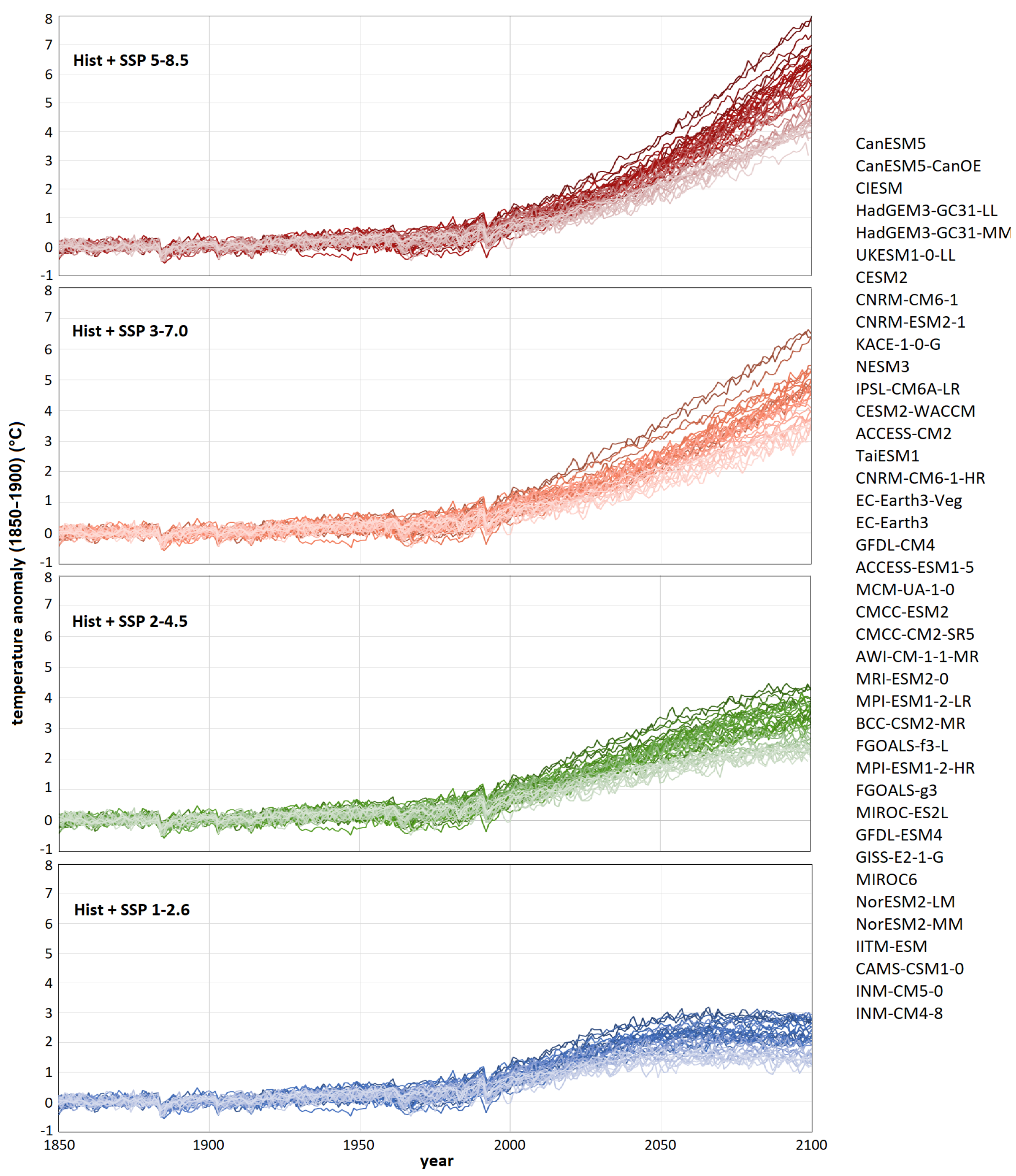
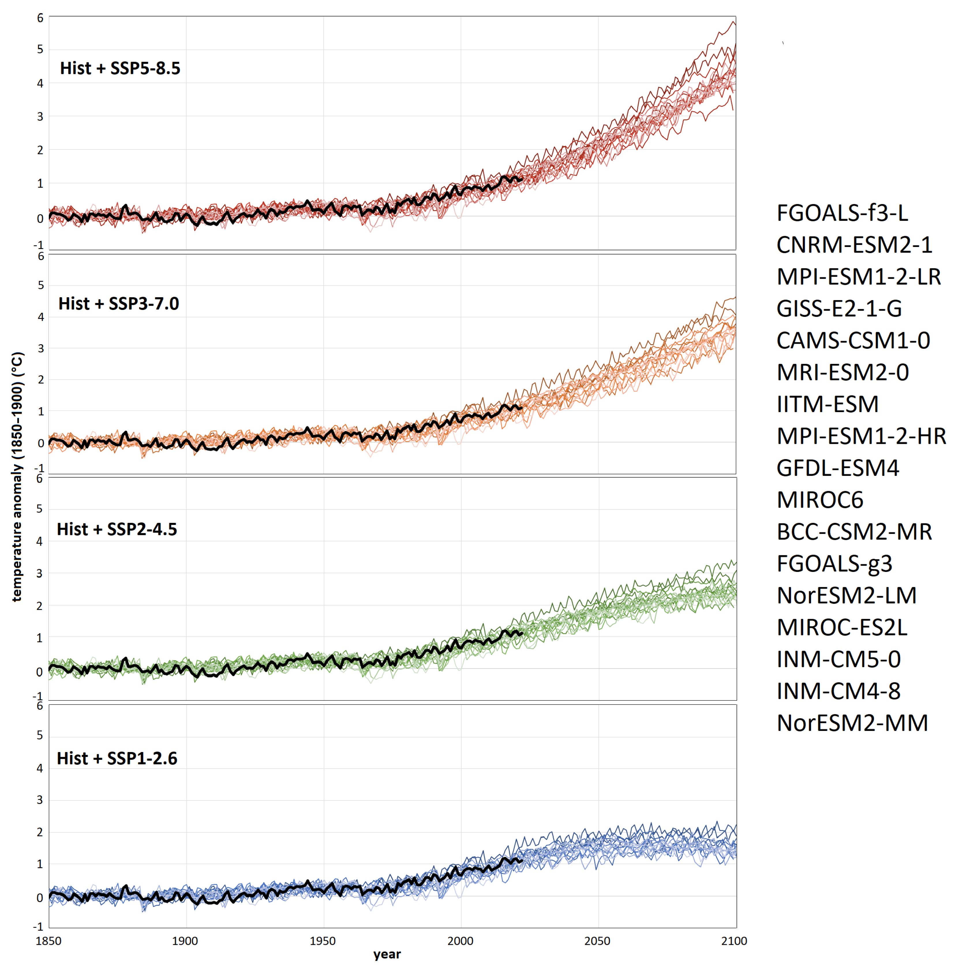
I additionally examine a selection of the surface air temperature (tas) simulations from 41 distinct CMIP6 GCMs obtained using historical forcings from 1850 to 2014 and four SSP forcing scenarios (SSP1-2.6, SSP2-4.5, SSP3-7.0, SSP5-8.5) from 2015 to 2100. The computer simulations for 37 GCMs were taken from the Supplemental Materials provided by Hausfather et al. [5]; those for other four GCMs (AWI-CM-1-1-MR, CNRM-CM6-1-HR, FGOALS-g3, and HadGEM3-GC31-MM) were downloaded from the KNMI Climate Explorer website. The total number of the examined synthetic temperature records was 152, which is more than what was previously analyzed by Scafetta [12,18]. See Figure 1.
This work does not repeat Scafetta [12]’s thorough analysis of the statistical implications of the models’ internal variability, which was found to have a modest effect. However, it should be noticed that here each GCM is represented by four simulations, which correspond to the four Hist + SSP scenarios when they are available. The differences among the four records partially reflect the dispersion caused by the internal variability of the models because the radiative forcing functions for the period from 1980 to 2022 do not differ significantly from one another.
The Equilibrium Climate Sensitivity (ECS) and Transient Climate Response (TCR) values of the CMIP6 Global Circulation Models (GCMs) were taken from the Table 7.SM.5 of the IPCC AR6 [3] and from the Supplementary Information of Hausfather et al. [5]. The two sets vary slightly: see Table A1.
The analytical method that is being suggested is comparable to Scafetta [12,18]’s. I will attempt to identify the three best subsets of GCMs that fall into the low, medium, and high ranges of ECS and TCR values. Then, I examine the temperature changes between 1980–1990 and 2011–2021 for model validation purposes, and the temperature changes between 1850–1899, 2045–2055, and 2090–2100 predicted by these three GCM subsets models for constraining realistic global aggregated impact and risk assessments.
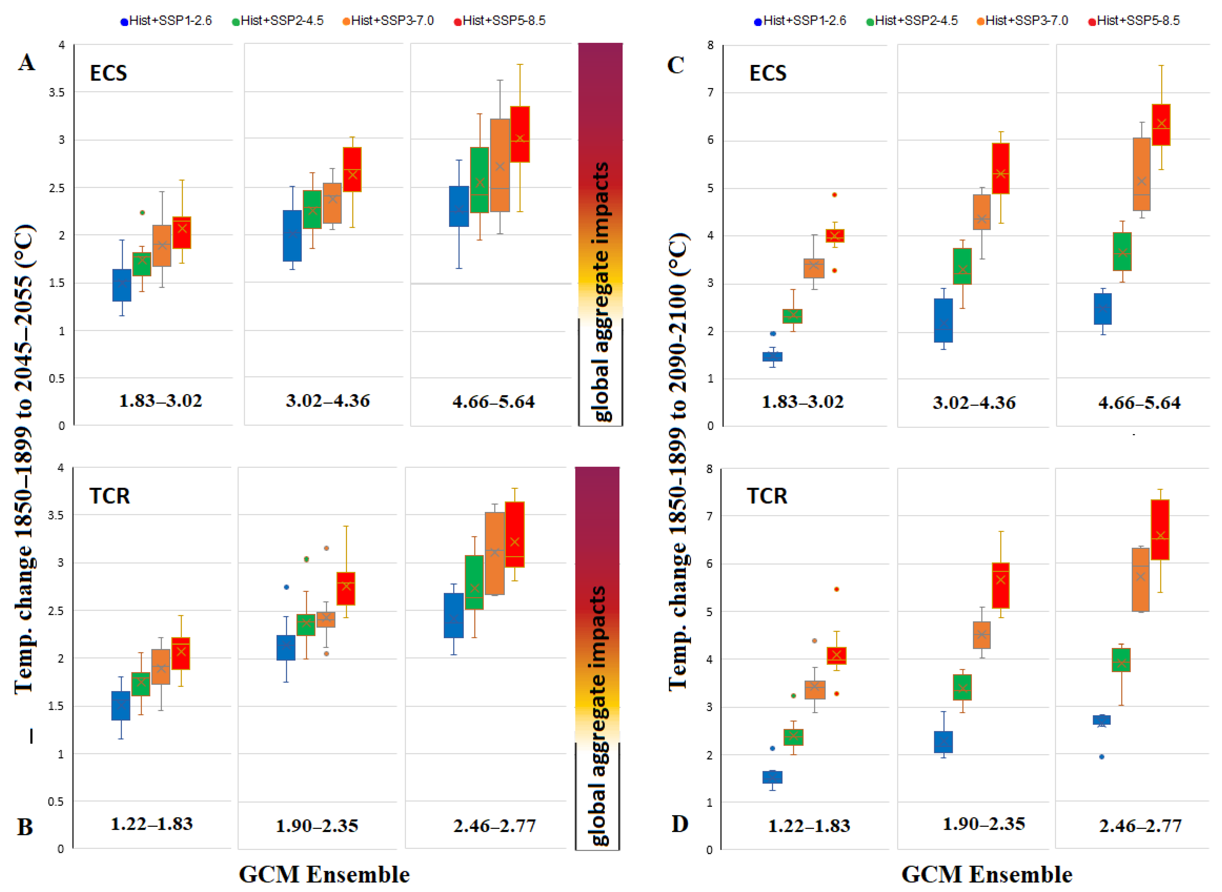
3. Results

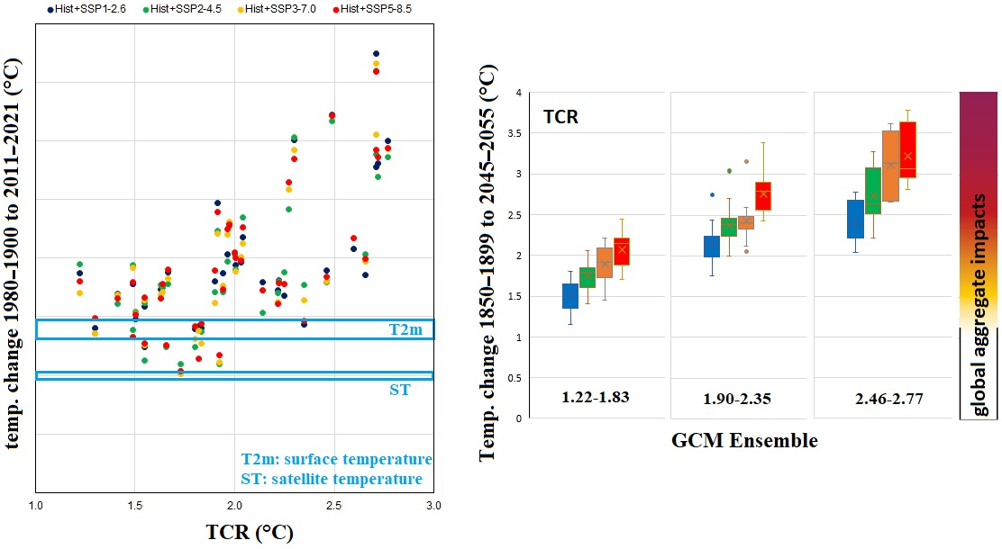
Figure 1 shows the CMIP6 GCM simulations that are being examined. Low-ECS (light color) and high-ECS models (dark color) alternate in the gradient of the curves’ hues. Each panel displays simulations made with different SSP forcing functions. The four panels unmistakably demonstrate that, as ECS increases, the models often forecast more warming for the twenty-first century.
Table A1 lists the names of the 41 CMIP6 GCM models with their Equilibrium Climate Sensitivity (ECS) and Transient Climate Response (TCR) values of the CMIP6 Global Circulation Models (GCMs). The ECS-150 and TCR records suggested by Hausfather et al. [5] appear to be the most comprehensive and will be the preferred ECS and TCR values for the upcoming statistics and tables.
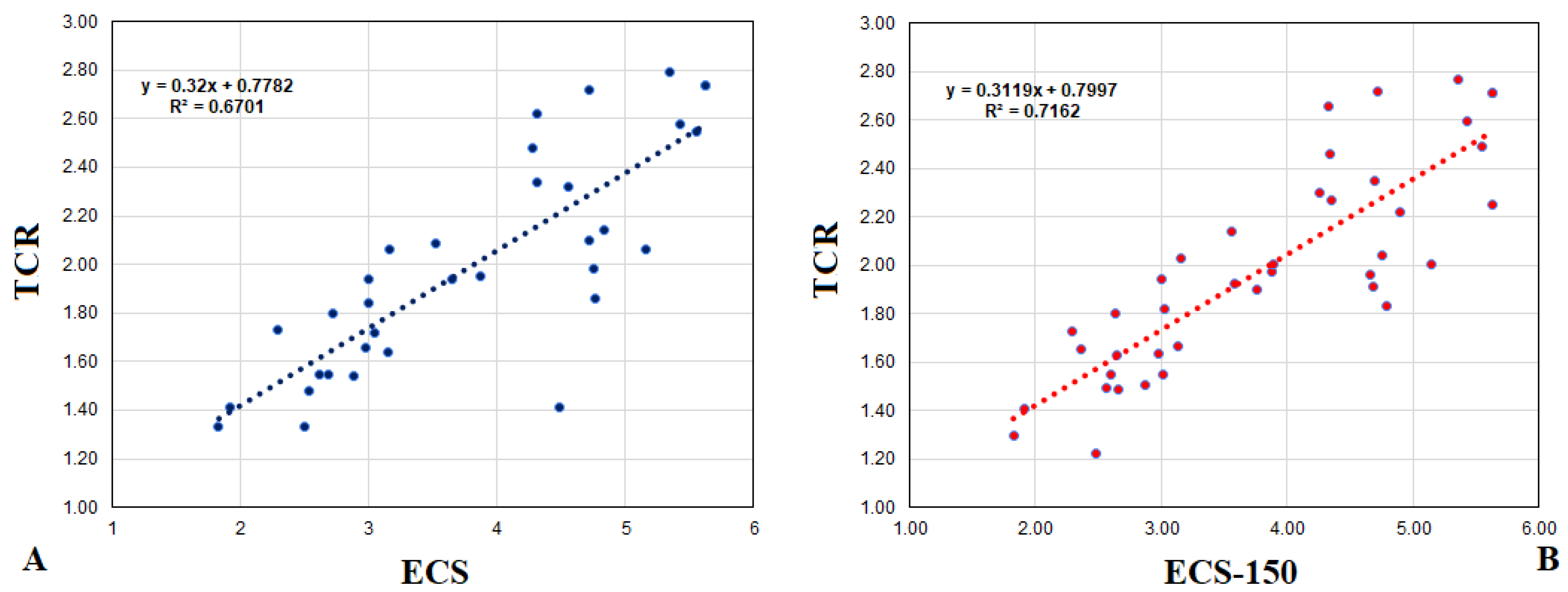
Figure 2 compares the ECS versus TCR values of the CMIP6 Global Circulation Models (GCMs). Figure 2A uses the data listed in the AR6 Table 7.SM.5 [3]. Figure 2B uses the data listed in the Supplementary Information of Hausfather et al. [5]. The regression analysis presented in the figure demonstrates a positive correlation between ECS and TCR, indicating that when ECS increases, TCR increases as well. The IPCC records, however, contain an anomaly for KACE-1-0-G that exhibits an exceptionally low TCR despite a high ECS (panel A) (ECS = 4.48 ° C, TCR = 1.41 ° C). These apparently anomalous values seem to have been corrected in Hausfather et al. [5] (KACE-1-0-G: ECS = 4.75 ° C, TCR = 2.04 ° C).
Figure 3 displays the temperature changes for the CMIP6 Global Circulation Models (GCMs) from 1980–1990 to 2011–2021 using panel (A), the ECS–150 values, and panel (B), the TCR values, from Hausfather et al. [5]. Table A2 summarizes the information for each model. Cyan boxes represent the warming ranges shown by the global surface temperature records (T2m), from 0.52 to 0.59 ° C, and by the lower troposphere UAH-MSU-lt v6 record (ST), from 0.39 to 0.41 ° C. Figure 3A largely replicates the outcomes reported by Scafetta [12,18], with a few minor variations.
The radiative forcing functions (Hist+SSP scenarios) throughout the studied period (1980–2021) are almost equal, and the variations in the simulations for the four SSP scenarios for each model roughly reflect the internal variability of the models themselves, as also noted by Scafetta [12,18]. Thus, Figure 3 and Table A2 demonstrate that the performance of the models dramatically declines as ECS or TCR rise. Generally speaking, only the sub-ensembles of GCMs with low-ECS and low-TCR GCM seem to fit the observations best.
CNRM-ESM2-1 and IPSL-CM6A-LR are two high-ECS models that seem to match the global surface temperature record from 1980 to 2021. However, CNRM-ESM2-1 appears to match the data because it has a low TCR despite having a high ECS (ECS = 4.79 ° C, TCR = 1.83 ° C). IPSL-CM6A-LR seems to be a bit of an outlier (ECS = 4.70 ° C, TCR = 2.35 ° C).
Figure 3 also demonstrates that if the lower troposphere UAHMSU-lt (ST) more closely mimics the actual warming, almost all GCMs would have overpredicted the warming from 1980–1990 to 2011–2021. In this case, CAMS-CSM1-0 (ECS = 2.29 ° C, TCR = 1.73 ° C) would be the only model that seems to match the temperature data.
Figure 3 suggests that, in accordance with low, medium, and high ECS and TCR ranges, the CMIP6 models can be divided into low, medium, and high climate sensitivity groups. However, only the low-sensitivity GCM sub-ensemble appears to best suit the surface temperature data and might be utilized for policy. The three ranges could be chosen as: low-ECS 1.83–3.02 ° C, low-TCR 1.22–1.83 ° C; medium-ECS 3.02–4.36 ° C, medium-TCR 1.90–2.35 ° C; high-ECS 4.66–5.64 ° C, high-TCR 2.46–2.77 ° C.
Table A3 and Table A4 report the temperature change from 1850–1899 to 2045–2055 and 2090–2100, respectively, for the CMIP6 Global Circulation Models (GCMs) using the ranking of the ECS-150 and TCR values from Hausfather et al. [5]. The tables show that the warming hindcasted by the models increases along with an increase in ECS and TCR. The Min–Max intervals for each of the three ECS sub-ensembles are listed in Table A5 for the four Hist + SSP scenarios and for the temperature change from 1850 to 1899 to 2045 to 2055 and 2090 to 2100 that were produced using the CMIP6 GCMs. Figure 4 shows the same warming ranges using boxplots that also demonstrates that the TCR-based ranges tend to be better separated from one another, supporting the possibility that a TCR-based selection could be better suitable than the ECS-based one.

4. Are the Global Surface Temperature Records Warm Biased?

This section briefly addresses why it might be conceivable that the recommended global surface temperature records frequently cited in scientific publications might exaggerate the global surface warming that has happened since the 1960s. If a large warm bias is actually present, then all CMIP6 GCMs (even those with low ECS and TCR values) should be dismissed for developing reliable climate change policy for the twenty-first century, as also McKitrick and Christy [7] concluded. Alternative climate data do, in fact, imply that there may be cause to doubt the extent of the real global surface warming that the Earth has undergone over the last century. Let us discuss a few of them now.

4.1. Comparison with the Lower Troposphere Temperature Record

The lower troposphere UAH-MSU record [29] shows a significantly lower warming (by about 0.2 ° C) from 1980–1990 to 2011–2021 than the HadCRUT5.0 (infilled data) [22]: see Figure 5A. It should be noticed that, according to the GCMs predictions, the global surface warming trend should be lower, and not higher, than in the troposphere [7,8]. In fact, the GCMs contend that surface warming is caused by back-radiation from greenhouse gases, which first warm the atmosphere. The UAH-MSU-lt record better correlates with the global warming trend obtained with 564 stations of the Integrated Global Radiosonde Archive (IGRA) dataset [33], as well as with sub-sections and with reanalysis datasets [34]. This result may make the UAH-MSU-lt record more reliable than alternative satellite temperature reconstructions, such as Remote Sensing Systems v4.0 (RSSv4.0) [35], NOAAv4.0 [36] and the University of Washington v1.0 (UWv1.0) [37].
Spencer et al. [29] explained that the different warming trend among the satellite composite records derived from the adjustments applied to the raw satellite data to create a reliable composite. For example, during the overlapping periods, biases could be detected in the results from earlier NOAA-11 through NOAA-14 experiments. The need for corrections appeared even more evident during the overlapping between NOAA-14 and NOAA-15 from late 1998 through 2004. NOAA-15 measurements were based on the novel Advanced MSU (AMSU) instruments. Thus, the UAH team decided to ignore NOAA-14 when the divergence from NOAA-15 became too evident. Spencer [38] stated that the other teams, instead, choose to “continue to use all of the NOAA-14 data through its entire lifetime and treat it as just as accurate as NOAA-15 AMSU data. Since NOAA-14 was warming significantly relative to NOAA-15, this puts a stronger warming trend into their satellite datasets, raising the temperature of all subsequent satellites’ measurements after about 2000”. As a result, the warming trend of UAH-MSU-lt may be plausible or at the very least, should be taken into consideration (e.g., as a lower limit).
If the UAH-MSU-lt record is correct, both the ECS and TCR low ranges given above (1.83–3.02 ° C and 1.22–1.83 ° C, respectively) should be reduced by about one-third; that is, 1.22–2.01 ° C and 0.81–1.22 ° C, respectively. Actually, using the UAH-MSU-lt record from 1979 to 2017, Christy and McNider [39] estimated that the (lower tropospheric) transient climate response (TCR) should be equal to 1.10 ± 0.26   ° C, which well agrees with the 0.81–1.22 ° C range. This low TCR estimate would be rather significant because it falls below both the AR6 likely range (1.4 to 2.2 ° C) and their very likely range (1.2 to 2.4 ° C).

4.2. Urban Heat Island and Other Non-Climatic Warm Biases

Long-term increases in Urban Heat Island effects, other local environmental changes, and instrumental degradation might have tainted a significant portion of the land temperature datasets. The scientific literature discusses evidence of possible warm biases; for example, see the references [27,28,40,41,42,43,44,45] and their citations. Connolly et al. [27], for instance, demonstrated that global surface temperature reconstruction for the Northern Hemisphere based on data from rural weather stations alone exhibits less warming (up to about 0.5 ° C in 2017) than the temperature records based on both rural and urban stations: see Figure 5B. Scafetta [28] demonstrated that, even after homogenization corrections, the global land surface temperature record (CRU TS4) presents large geographical areas that exhibit abnormally high nighttime warming in contrast to daytime temperatures. For example, Scafetta and Ouyang [40] showed that for China, the daytime summer temperature ( T M a x ) record indicates that the 2005–2015 period was as warm as 1940–1950, whereas the winter nighttime temperature ( T M i n ) showed significant warming. These results are proof of a warming that originates at the surface that, during the daytime, is fast dissipated vertically because the capping inversion layer is usually relatively high from the surface, whereas, during the nighttime, it is more dissipated horizontally because the capping inversion layer is usually relatively low from the surface. Thus, the heat trapped at the surface during the day is, during the night, more easily spread around, which is what is usually observed in urban areas. The bias in the temperature records, in particular, overnight, occurs because of the growth of the cities, which makes the surrounding warmer and warmer: see also the recent study by Kim and Christy [45]. Moreover, the weather stations are affected by many other issues that could induce a warm bias, as documented by D’Aleo [42] and Watts [41]. Temperature homogenization algorithms could then blend some warming from urban to rural regions, skewing the final climatic record [27].
Figure 5. Evidence suggesting that the global surface temperature records (red curves) may be warm biased, in particular, over land. (A) Divergence between HadCRUT5 (infilled data, red) [22] and the UAH-MSU-lt 6.0 [29] temperature records (blue). (B) Divergence between Northern Hemisphere land temperature records using urban and rural stations (red) and rural only stations (blue), from Connolly et al. [27]. (C,D) compare the CRUTEM 5.0 (land) [46] and the HadSST4 (ocean) [47] records versus the land and the ocean records of UAH-MSU-lt v. 6.0 [29], respectively; the UAH-MSU-lt records were baselined with the surface records in the period 1980–1990. (E) Divergence between the summer (JJA) instrumental temperatures averaged over 30 ° N–70 ° N land areas (red) and the tree-based mean temperature reconstructions (blue) relative to the 1930–1960 period [48]. (F) Divergence among the HadCRUT3 (1850–2014), HadCRUT4 (1850–2021), HadCRUT5 (non-infilled data, 1850–2021), and HadCRUT5 (infilled data, 1850–2021) global surface temperature records relative to the 1850–1900 period.
Atmosphere 14 00345 g005

4.3. The Land Warms Too Much More Than the Ocean

The IPCC [3] stated that from 1850–1900 to 2011–2020 the mean warming over the ocean was 0.88 °C and that over land was nearly double, that it 1.59 °C. However, from about 1970 to 2022, the land area appears to have warmed up too fast and too much relative to the ocean region. This is shown in Figure 5C,D that compares the CRUTEM 5.0 (land) [46] and the HadSST4 (ocean) [47] records versus the land and the ocean records of UAH-MSU-lt 6.0 [29], respectively. From 1980–1990 to 2015–2022, over land, the UAH-MSU-lt warmed 0.65 °C, and over the ocean, it warmed 0.44 °C: this land/ocean ratio is 1.48. However, the land surface record (CRUTEM) warmed by around 0.96 ° C, whereas the sea surface temperature (HadSST4) warmed by about 0.53 ° C: this land/ocean ratio is 1.81. It should be noticed that 1.81 is 22% larger than 1.48. Moreover, HadSST4 is 0.09 °C (20%) warmer than the satellite estimate, whereas CRUTEM is 0.31 °C (48%) warmer than UAH-MSU-lt. These large differences suggest the presence of possible warm biases in the land record. See also the in-depth analysis by Scafetta [12,28], which demonstrated that, in contrast to the ocean warming, the CMIP6 GCMs also hindcast, in percentage, lesser terrestrial warming than what was reported by the surface temperature records.

4.4. The “Divergence Problem” with the Tree-Ring-Width Chronologies

There exists a so-called “divergence problem”, which is the apparent decoupling between proxy temperature records based on tree-ring-width chronologies and the rising temperature data from land stations starting in the 1970s. See Figure 5E. This decoupling may potentially give indirect evidence for the existence of a considerable warming bias in the station-based temperature records (up to about 0.5 ° C in 2000), especially over land [28,48,49]. The global surface temperature reconstruction for the Northern Hemisphere based on data from rural weather stations alone (shown in Figure 5B) is roughly compatible with the significantly less warming inferred from the tree ring chronologies for the years 1970 to 2000.

4.5. Doubts Regarding the Global Surface Temperature Revised Records

The most recent revisions of the global surface temperature records may have used inappropriate temperature homogenization models that have artificially blended urban warming toward rural areas and may have filled uncovered areas (e.g., the polar regions) with overly warm model temperature predictions. Indeed, all surface and satellite climate records available before 2014 (e.g., HadCRUT3, which was discontinued in 2014 [50]) showed more than a decade of relatively little change; the scientific community has actually labeled the years 2000 to 2014 as a “pause” or “hiatus” in global warming [2]. However, during the last few years, from one climate version to the next, the 2000–2014 “pause” has gradually disappeared and was substituted by an increasingly strong warming trend. For example, the trend was 0.03 ° C/decade for HadCRUT3, and became 0.08 ° C/decade for HadCRUT4 [51], 0.10 ° C/decade for HadCRUT5 non-infilled data, and 0.14 ° C/decade for HadCRUT5 infilled data [22]. See Table A6 and Figure 5F. However, the UAH-MSU-lt v6 record, which shows a warming trend of 0.012 ° C/decade from 2000 to 2014, nonetheless confirms the existence of a global warming “hiatus” during the same period. Also the NH rural-only stations temperature record shown in Figure 5B and the HadSST4 (ocean) record shown in Figure 5D appear to confirm the existence of a global warming hiatus from 2000 to 2014.

4.6. Natural Climate Variability and Oscillations

Several studies have shown that multidecadal and millennial natural oscillations may significantly influence the climate system [11,30,31,52]. Some of these natural oscillations may be explained by more appropriate solar and/or astronomical forcing functions than those used to force the CMIP6 GCMs [27,53,54]. Large climatic natural oscillations for the multidecadal to the millennial scales that are not reproduced by the models would suggest that the ECS of GCMs should be reduced by at least a factor of two [11,30,31,32] and might vary between 0.9 and 3.0 ° C, if all CMIP6 GCMs are considered, or between 0.9 and 1.5 ° C, if only the low-ECS models are considered, which would confirm the results from several authors [17,30,32,55,56,57,58,59]. Moderating near-future climate projections is the most immediate impact of natural multidecadal climate oscillations [11,30,31,60]. In fact, the ECS and the importance of rising CO2 in climate change forecasts would be greatly overstated if any natural source of global climate warming, particularly that brought on by multidecadal, secular and millennial climatic cycles, is disregarded by the GCMs.

5. Discussion and Conclusions

The low ECS and TCR GCM sub-ensembles seem to be the group that does the greatest job in hindcasting the warming reported from 1980–1990 to 2011–2021 by the global surface temperature records usually used to assess global warming, as shown in Figure 3.
The decision to adopt a specific metric (the global temperature change from 1980–1990 to 2011–2021) to assess GCM performance was not arbitrary. It considered the time period with the lowest statistical uncertainty in the data, the availability of alternative temperature records (such as the satellite ones for an indirect comparison), the potential implication for long-range oscillating patterns (such as the effect of a quasi 60-year cycle [30,32,52,60]), and the fact that the global surface temperature is the most significant global climatic index, which is also directly related to the global aggregated impact and risk assessments assuming low to no adaptation [1]. Additionally, it may be fair to select models that better predict historical global warming when formulating policies to address the risks associated with climate change in the coming decades.
The model hindcasts appear to fail for the GCM sets with both the medium and high ECS or TCR, making these models inappropriate for directing climate change policy to address future climate change dangers. A TCR-based choice might even be more appropriate, as shown in Figure 4. The findings suggest that a GCM sub-ensemble comprised of 14 low-ECS GCMs (1.83–3.02 ° C) or 16 low TCR GCMs (1.22–1.83 ° C) on the 41 examined CMIP6 GCMs could be employed most effectively for climate change policy.
By merging the two sets, the best performing GCM sub-ensemble should be made of 17 GCMs, which are: FGOALS-f3-L, CNRM-ESM2-1, MPI-ESM1-2-LR, GISS-E2-1-G, CAMS-CSM1-0, MRI-ESM2-0, IITM-ESM, MPI-ESM1-2-HR, GFDL-ESM4, MIROC6, BCC-CSM2-MR, FGOALS-g3, NorESM2-LM, MIROC-ES2L, INM-CM5-0, INM-CM4-8, and NorESM2-MM. The average simulations by these 17 GCMs are depicted in Figure 6.
Table A5 and Figure 4 demonstrate how choosing GCM sub-ensembles significantly affects the GCM predicted warming for the 21st century. For example, by using the Hist-SSP2-4.5 and Hist-SSP3-7.0 scenarios and selecting the low-ECS range, the predicted warming for 2045–2055 varies from 1.41 to 2.46 ° C; selecting the medium-ECS range, the predicted warming for 2045–2055 varies from 1.85 to 2.68 ° C; and selecting the high-ECS range, the predicted warming for 2045–2055 varies from 1.95 to 3.61 ° C. Similarly, by selecting the low-TCR range, the predicted warming for 2045–2055 varies from 1.41 to 2.21 ° C; selecting the medium-TCR range, the predicted warming for 2045–2055 varies from 2.00 to 3.15 ° C; and selecting the high-TCR range, the predicted warming for 2045–2055 varies from 2.22 to 3.61 ° C.
These differences are significant because local climate adaptation strategies should be adequate to manage any form of climate change danger if the expected warming for 2045–2055 is, let us say, 1.4–2.5 °C [1]. This result is also confirmed in Figure 4, which also shows the global aggregated impact and risk assessments assuming low to no adaptation [1]. This risk scale measures the impacts on socio-ecological systems that can be aggregated globally into a single metric, such as monetary damages, lives affected, species lost, or ecosystem degradation at a global scale.
However, a crucial issue is still open. If the lower troposphere UAH-MSU-lt v6 record more precisely reproduces the warming that really happened from 1980 to 2021, then the only CMIP6 model that would seem to fit the temperature data would be CAMS-CSM1-0 (ECS = 2.29 ° C, TCR = 1.73 ° C). In general, all of the CMIP6 GCMs seem to have a persistent warming bias in the tropospheric layers [7,8] and, actually, they fail in many climatic hindcasts (e.g. they poorly reproduce the Northern Hemisphere snow-cover trends from 1967 to 2018 [61]). In this situation, all the CMIP6 GCMs would be inadequate and even misleading to serve as a guide for climate change policies for the twenty-first century because to agree with the actual observations, the low ECS or TCR GCM simulations should be reduced, on average, by one-third, which would also drastically reduce their warming forecasts for the 21st century and, consequently, the relative climatological risk assessments [12].
Finally, Section 4 discusses a few points that could call into doubt how much the global surface temperature has been warming. In fact, there are several indications that a global warming has really taken place during the past 150 years, albeit it may have been less than the 1.09 °C indicated by the official global surface temperature data from 1850–1900 to 2011–2020 [3]. The reported warming may have been overestimated due to urban heat biases and other local influences that might have skewed the data [27,28,40]. The presented evidences briefly discuss and compare the global surface temperature records against a number of alternative temperature reconstructions from lower troposphere satellite measurements, tree-ring-width chronologies, and surface temperature records based on rural stations alone. Thus, it is possible, as claimed by McKitrick and Christy [7], that the actual ECS and TCR could be lower than what is simulated by the CMIP6 GCMs. Very low ECS and TCR values (around 0.5–2.0 ° C) are actually suggested by some authors [30,32,56,57,58,59], and this eventuality should be further investigated. If true, new climate models could be required to develop reliable climate change policies for the twenty-first century.

Supplementary Materials

The following are available online at https://www.mdpi.com/article/10.3390/atmos14020345/s1, The attached file manuscript-supplementary.xlsx collects the CMIP6 GCM simulations adopted in this study.

Funding

This research received no external funding.

Data Availability Statement

Conflicts of Interest

The author declares no conflict of interest.

Appendix A

Table A1. Equilibrium Climate Sensitivity (ECS) and Transient Climate Response (TCR) of the CMIP6 Global Circulation Models (GCMs).
Model NameECS 1TCR 1ECS-150 2ECS-130 2TCR 2
( ° C)( ° C)( ° C)( ° C)( ° C)
ACCESS-CM24.722.104.665.401.96
ACCESS-ESM1-53.871.953.884.901.97
AWI-CM-1-1-MR3.162.063.163.292.03
BCC-CSM2-MR3.041.723.023.501.55
CAMS-CSM1-02.291.732.292.311.73
CESM25.162.065.156.432.00
CESM2-WACCM4.751.984.685.491.91
CIESM 2.395.636.332.25
CMCC-CM2-SR53.522.093.563.532.14
CMCC-ESM2 3.583.551.92
CNRM-CM6-14.832.144.904.762.22
CNRM-CM6-1-HR4.282.484.344.072.46
CNRM-ESM2-14.761.864.794.901.83
CanESM55.622.745.645.762.71
CanESM5-CanOE5.622.745.645.762.71
EC-Earth3 2.304.26 2.30
EC-Earth3-Veg4.312.624.334.452.66
FGOALS-f3-L31.943.00 1.94
FGOALS-g32.881.542.873.101.50
FIO-ESM-2-0 2.22 2.22
GFDL-CM4 3.894.402.00
GFDL-ESM4 2.652.631.63
GISS-E2-1-G2.721.802.642.631.80
HadGEM3-GC31-LL5.552.555.555.732.49
HadGEM3-GC31-MM5.422.585.435.352.60
IITM-ESM 1.712.372.421.66
INM-CM4-81.831.331.831.911.30
INM-CM5-01.92 1.922.021.41
IPSL-CM6A-LR4.562.324.705.182.35
KACE-1-0-G4.481.414.75 2.04
MCM-UA-1-03.651.943.763.971.90
MIROC-ES2L2.681.552.662.531.49
MIROC62.611.552.602.591.55
MPI-ESM1-2-HR2.981.662.983.341.64
MPI-ESM1-2-LR31.843.023.081.82
MRI-ESM2-03.151.643.133.421.67
NESM34.722.724.72 2.72
NorESM2-LM2.541.482.562.981.49
NorESM2-MM2.51.332.492.681.22
TaiESM14.312.344.364.682.27
UKESM1-0-LL5.342.795.365.492.77
1 Data from IPCC [3] AR6, Table 7.SM.5. 2 Data from Supplementary Information of Hausfather et al. [5].
Table A2. Temperature change from 1980–1990 to 2011–2021 for the CMIP6 Global Circulation Models (GCMs). Ranking using ECS-150 and TCR from Hausfather et al. [5]. See Figure 3.
Model NameECS-150Hist+Hist+Hist+Hist+ Model NameTCRHist+Hist+Hist+Hist+
1–2.62–4.53–7.05–8.5 μ ± σ 1–2.62–4.53–7.05–8.5 μ ± σ
( ° C)( ° C)( ° C)( ° C)( ° C)( ° C) ( ° C)( ° C)( ° C)( ° C)( ° C)( ° C)
CanESM55.641.501.441.461.441.46 ± 0.02UKESM1-0-LL2.771.201.151.171.181.17 ± 0.02
CIESM5.630.670.75 0.710.71 ± 0.03NESM32.721.121.08 1.151.12 ± 0.03
HadGEM3-GC31-LL5.551.291.27 1.291.28 ± 0.01CanESM52.711.501.441.461.441.46 ± 0.02
HadGEM3-GC31-MM5.430.83 0.870.85 ± 0.02CanESM5-CanOE2.711.111.151.221.171.16 ± 0.04
UKESM1-0-LL5.361.201.151.171.181.17 ± 0.02EC-Earth3-Veg2.660.740.810.790.800.79 ± 0.03
CanESM5-CanOE5.361.111.151.221.171.16 ± 0.04HadGEM3-GC31-MM2.600.83 0.870.85 ± 0.02
CESM25.150.780.760.760.800.77 ± 0.02HadGEM3-GC31-LL2.491.291.27 1.291.28 ± 0.01
CNRM-CM6-14.900.690.680.650.640.67 ± 0.02CNRM-CM6-1-HR2.460.760.720.720.740.73 ± 0.02
CNRM-ESM2-14.790.560.550.510.580.55 ± 0.03IPSL-CM6A-LR2.350.570.710.660.580.63 ± 0.06
KACE-1-0-G4.750.870.940.850.910.89 ± 0.03EC-Earth32.301.201.211.171.141.18 ± 0.03
NESM34.721.121.08 1.151.12 ± 0.03TaiESM12.27 0.971.031.061.02 ± 0.04
IPSL-CM6A-LR4.700.570.710.660.580.63 ± 0.06CIESM2.250.670.75 0.710.71 ± 0.03
CESM2-WACCM4.680.990.890.890.960.93 ± 0.04FIO-ESM-2-02.220.720.72 0.710.72 ± 0.00
ACCESS-CM24.660.810.790.880.900.85 ± 0.05CNRM-CM6-12.220.690.680.650.640.67 ± 0.02
TaiESM14.36 0.971.031.061.02 ± 0.04CMCC-CM2-SR52.140.720.610.690.690.68 ± 0.04
CNRM-CM6-1-HR4.340.760.720.720.740.73 ± 0.02KACE-1-0-G2.040.870.940.850.910.89 ± 0.03
EC-Earth3-Veg4.330.740.810.790.800.79 ± 0.03AWI-CM-1-1-MR2.030.790.800.800.790.79 ± 0.01
EC-Earth34.261.201.211.171.141.18 ± 0.03CESM22.000.780.760.760.800.77 ± 0.02
GFDL-CM43.89 0.81 0.820.82 ± 0.00GFDL-CM42.00 0.81 0.820.82 ± 0.00
ACCESS-ESM1-53.880.920.910.920.910.92 ± 0.01ACCESS-ESM1-51.970.920.910.920.910.92 ± 0.01
MCM-UA-1-03.760.720.680.650.760.70 ± 0.04ACCESS-CM21.960.810.790.880.900.85 ± 0.05
CMCC-ESM23.58 0.440.440.470.45 ± 0.01FGOALS-f3-L1.940.750.690.710.690.71 ± 0.02
CMCC-CM2-SR53.560.720.610.690.690.68 ± 0.04CMCC-ESM21.92 0.440.440.470.45 ± 0.01
AWI-CM-1-1-MR3.160.790.800.800.790.79 ± 0.01CESM2-WACCM1.910.990.890.890.960.93 ± 0.04
MRI-ESM2-03.130.750.710.730.760.74 ± 0.02MCM-UA-1-01.900.720.680.650.760.70 ± 0.04
BCC-CSM2-MR3.020.640.650.660.670.65 ± 0.01CNRM-ESM2-11.830.560.550.510.580.55 ± 0.03
MPI-ESM1-2-LR3.020.570.550.550.460.53 ± 0.04MPI-ESM1-2-LR1.820.570.550.550.460.53 ± 0.04
FGOALS-f3-L3.000.750.690.710.690.71 ± 0.02GISS-E2-1-G1.800.560.500.530.570.54 ± 0.03
MPI-ESM1-2-HR2.980.700.700.680.710.70 ± 0.01CAMS-CSM1-01.730.420.440.410.410.42 ± 0.01
FGOALS-g32.870.590.620.610.610.61 ± 0.01MRI-ESM2-01.670.750.710.730.760.74 ± 0.02
MIROC-ES2L2.660.530.560.530.530.54 ± 0.01IITM-ESM1.66 0.50 0.500.50 ± 0.00
GFDL-ESM42.650.690.710.680.660.69 ± 0.02MPI-ESM1-2-HR1.640.700.700.680.710.70 ± 0.01
GISS-E2-1-G2.640.560.500.530.570.54 ± 0.03GFDL-ESM41.630.690.710.680.660.69 ± 0.02
MIROC62.600.500.450.500.510.49 ± 0.02MIROC61.550.500.450.500.510.49 ± 0.02
NorESM2-LM2.560.710.770.770.720.74 ± 0.03BCC-CSM2-MR1.550.640.650.660.670.65 ± 0.01
NorESM2-MM2.490.750.780.680.720.73 ± 0.04FGOALS-g31.500.590.620.610.610.61 ± 0.01
IITM-ESM2.37 0.50 0.500.50 ± 0.00NorESM2-LM1.490.710.770.770.720.74 ± 0.03
CAMS-CSM1-02.290.420.440.410.410.42 ± 0.01MIROC-ES2L1.490.530.560.530.530.54 ± 0.01
INM-CM5-01.920.680.640.680.660.67 ± 0.01INM-CM5-01.410.680.640.680.660.67 ± 0.01
INM-CM4-81.830.560.540.540.600.56 ± 0.02INM-CM4-81.300.560.540.540.600.56 ± 0.02
NorESM2-MM1.220.750.780.680.720.73 ± 0.04
Table A3. Temperature change from 1850–1899 to 2045–2055 for the CMIP6 Global Circulation Models (GCMs). The ranking uses ECS-150 and TCR from Hausfather et al. [5].
Model NameECS150Hist+Hist+Hist+Hist+Model NameTCRHist+Hist+Hist+Hist+
SSP1-2.6SSP2-4.5SSP3-7.0SSP5-8.5 SSP1-2.6SSP2-4.5SSP3-7.0SSP5-8.5
( ° C)( ° C)( ° C)( ° C)( ° C) ( ° C)( ° C)( ° C)( ° C)( ° C)
CanESM55.642.743.083.443.74UKESM1-0-LL2.772.442.793.133.34
CanESM5-CanOE5.642.773.283.613.78NESM32.722.032.22 2.81
CIESM5.632.112.71 3.05CanESM52.712.743.083.443.74
HadGEM3-GC31-LL5.552.292.61 3.12CanESM5-CanOE2.712.773.283.613.78
HadGEM3-GC31-MM5.432.29 3.00EC-Earth3-Veg2.662.192.512.683.01
UKESM1-0-LL5.362.442.793.133.34HadGEM3-GC31-MM2.602.29 3.00
CESM25.152.162.252.282.79HadGEM3-GC31-LL2.492.292.61 3.12
CNRM-CM6-14.901.792.002.112.43CNRM-CM6-1-HR2.462.502.642.662.94
CNRM-ESM2-14.791.651.952.012.25IPSL-CM6A-LR2.352.242.382.602.94
KACE-1-0-G4.752.753.043.153.38EC-Earth32.302.042.232.392.70
NESM34.722.032.22 2.81TaiESM12.27 2.392.422.94
IPSL-CM6A-LR4.702.242.382.602.94CIESM2.252.112.71 3.05
CESM2-WACCM4.682.222.422.352.82FIO-ESM-2-02.222.202.49 2.81
ACCESS-CM24.662.262.392.392.64CNRM-CM6-12.221.792.002.112.43
TaiESM14.36 2.392.422.94CMCC-CM2-SR52.142.442.472.562.85
CNRM-CM6-1-HR4.342.502.642.662.94KACE-1-0-G2.042.753.043.153.38
EC-Earth3-Veg4.332.192.512.683.01AWI-CM-1-1-MR2.032.002.332.462.53
EC-Earth34.262.042.232.392.70CESM22.002.162.252.282.79
GFDL-CM43.89 2.06 2.47GFDL-CM42.00 2.06 2.47
ACCESS-ESM1-53.881.752.172.052.48ACCESS-ESM1-51.971.752.172.052.48
MCM-UA-1-03.762.122.292.442.88ACCESS-CM21.962.262.392.392.64
CMCC-ESM23.58 2.462.402.67FGOALS-f3-L1.941.952.242.462.58
CMCC-CM2-SR53.562.442.472.562.85CMCC-ESM21.92 2.462.402.67
AWI-CM-1-1-MR3.162.002.332.462.53CESM2-WACCM1.912.222.422.352.82
MRI-ESM2-03.131.802.062.212.44MCM-UA-1-01.902.122.292.442.88
BCC-CSM2-MR3.021.661.812.122.31CNRM-ESM2-11.831.651.952.012.25
MPI-ESM1-2-LR3.021.641.852.092.08MPI-ESM1-2-LR1.821.641.852.092.08
FGOALS-f3-L3.001.952.242.462.58GISS-E2-1-G1.801.771.881.902.16
MPI-ESM1-2-HR2.981.561.801.952.00CAMS-CSM1-01.731.181.501.591.71
FGOALS-g32.871.411.812.132.15MRI-ESM2-01.671.802.062.212.44
MIROC-ES2L2.661.621.751.862.15IITM-ESM1.66 1.79 2.14
GFDL-ESM42.651.421.591.731.92MPI-ESM1-2-HR1.641.561.801.952.00
GISS-E2-1-G2.641.771.881.902.16GFDL-ESM41.631.421.591.731.92
MIROC62.601.351.531.731.87MIROC61.551.351.531.731.87
NorESM2-LM2.561.151.411.451.74BCC-CSM2-MR1.551.661.812.122.31
NorESM2-MM2.491.261.661.621.86FGOALS-g31.501.411.812.132.15
IITM-ESM2.37 1.79 2.14NorESM2-LM1.491.151.411.451.74
CAMS-CSM1-02.291.181.501.591.71MIROC-ES2L1.491.621.751.862.15
INM-CM5-01.921.631.742.092.22INM-CM5-01.411.631.742.092.22
INM-CM4-81.831.511.801.922.18INM-CM4-81.301.511.801.922.18
NorESM2-MM1.221.261.661.621.86
Table A4. Temperature change from 1850–1899 to 2090–2100 for the CMIP6 Global Circulation Models (GCMs). Ranking using ECS-150 and TCR from Hausfather et al. [5].
Model NameECS150Hist+Hist+Hist+Hist+Model NameTCRHist+Hist+Hist+Hist+
SSP1-2.6SSP2-4.5SSP3-7.0SSP5-8.5 SSP1-2.6SSP2-4.5SSP3-7.0SSP5-8.5
(°C)(°C)(°C)(°C)(°C) (°C)(°C)(°C)(°C)(°C)
CanESM55.642.784.226.267.46UKESM1-0-LL2.772.734.195.947.00
CanESM5-CanOE5.642.834.316.367.56NESM32.721.943.02 5.38
CIESM5.632.183.79 6.69CanESM52.712.784.226.267.46
HadGEM3-GC31-LL5.552.743.92 6.60CanESM5-CanOE2.712.834.316.367.56
HadGEM3-GC31-MM5.432.79 6.42EC-Earth3-Veg2.662.573.735.026.06
UKESM1-0-LL5.362.734.195.947.00HadGEM3-GC31-MM2.602.79 6.42
CESM25.152.333.324.526.02HadGEM3-GC31-LL2.492.743.92 6.60
CNRM-CM6-14.902.053.224.575.91CNRM-CM6-1-HR2.462.803.924.986.17
CNRM-ESM2-14.792.133.224.375.46IPSL-CM6A-LR2.352.273.614.986.41
KACE-1-0-G4.752.893.675.086.02EC-Earth32.302.063.244.545.65
NESM34.721.943.02 5.38TaiESM12.27 3.794.876.02
IPSL-CM6A-LR4.702.273.614.986.41CIESM2.252.183.79 6.69
CESM2-WACCM4.682.453.334.526.07FIO-ESM-2-02.222.153.38 5.83
ACCESS-CM24.662.543.504.765.83CNRM-CM6-12.222.053.224.575.91
TaiESM14.36 3.794.876.02CMCC-CM2-SR52.142.903.744.385.59
CNRM-CM6-1-HR4.342.803.924.986.17KACE-1-0-G2.042.893.675.086.02
EC-Earth3-Veg4.332.573.735.026.06AWI-CM-1-1-MR2.031.942.994.194.97
EC-Earth34.262.063.244.545.65CESM22.002.333.324.526.02
GFDL-CM43.89 3.01 4.98GFDL-CM42.00 3.01 4.98
ACCESS-ESM1-53.882.003.114.134.86ACCESS-ESM1-51.972.003.114.134.86
MCM-UA-1-03.762.173.174.235.13ACCESS-CM21.962.543.504.765.83
CMCC-ESM23.58 3.684.365.49FGOALS-f3-L1.941.942.884.044.87
CMCC-CM2-SR53.562.903.744.385.59CMCC-ESM21.92 3.684.365.49
AWI-CM-1-1-MR3.161.942.994.194.97CESM2-WACCM1.912.453.334.526.07
MRI-ESM2-03.131.672.713.754.58MCM-UA-1-01.902.173.174.235.13
BCC-CSM2-MR3.021.502.543.834.14CNRM-ESM2-11.832.133.224.375.46
MPI-ESM1-2-LR3.021.642.473.524.28MPI-ESM1-2-LR1.821.642.473.524.28
FGOALS-f3-L3.001.942.884.044.87GISS-E2-1-G1.801.672.433.354.14
MPI-ESM1-2-HR2.981.532.413.544.17CAMS-CSM1-01.731.251.982.883.28
FGOALS-g32.871.402.263.493.80MRI-ESM2-01.671.672.713.754.58
MIROC-ES2L2.661.552.533.344.29IITM-ESM1.66 2.34 3.76
GFDL-ESM42.651.382.283.433.94MPI-ESM1-2-HR1.641.532.413.544.17
GISS-E2-1-G2.641.672.433.354.14GFDL-ESM41.631.382.283.433.94
MIROC62.601.402.183.103.99MIROC61.551.402.183.103.99
NorESM2-LM2.561.282.142.983.92BCC-CSM2-MR1.551.502.543.834.14
NorESM2-MM2.491.392.133.163.98FGOALS-g31.501.402.263.493.80
IITM-ESM2.37 2.34 3.76NorESM2-LM1.491.282.142.983.92
CAMS-CSM1-02.291.251.982.883.28MIROC-ES2L1.491.552.533.344.29
INM-CM5-01.921.492.403.403.88INM-CM5-01.411.492.403.403.88
INM-CM4-81.831.432.293.403.94INM-CM4-81.301.432.293.403.94
NorESM2-MM1.221.392.133.163.98
Table A5. Temperature change from 1850–1899 to 2045–2055 and 2090–2100 the CMIP6 Global Circulation Models (GCMs) for three ECS and TCR GCM ensembles and four SSP scenarios. See Figure 4.
GCM 1850–1899 to 2045–20551850–1899 to 2090–2100
Sub-Ensemble Hist-SSP1-2.6Hist-SSP2-4.5Hist-SSP3-7.0Hist-SSP5-8.5Hist-SSP1-2.6Hist-SSP2-4.5Hist-SSP3-7.0Hist-SSP5-8.5
ECS150(°C)(°C)(°C)(°C)(°C)(°C)(°C)(°C)(°C)
(3) high4.66–5.641.65–2.771.95–3.282.01–3.612.25–3.781.94–2.893.02–4.314.37–6.365.38–7.56
(2) medium3.02–4.361.64–2.501.85–2.642.05–2.682.08–3.011.64–2.902.47–3.923.52–5.024.28–6.17
(1) low1.83–3.021.15–1.951.41–2.241.45–2.461.71–2.581.25–1.941.98–2.882.88–4.043.28–4.87
TCR(°C)(°C)(°C)(°C)(°C)(°C)(°C)(°C)(°C)
(3) high2.46–2.772.03–2.772.22–3.282.66–3.612.81–3.781.94–2.833.02–4.314.98–6.365.38–7.56
(2) medium1.90–2.351.75–2.752.00–3.042.05–3.152.43–3.381.94–2.902.88–3.794.04–5.084.86–6.69
(1) low1.22–1.831.15–1.801.41–2.061.45–2.211.71–2.441.25–2.131.98–3.222.88–4.373.28–5.46
Table A6. Warming means and trends in various periods for HadCRUT3 (1850–2014), HadCRUT4 (1850–2021), HadCRUT5 (non-infilled data, 1850–2021), and HadCRUT5 (filled data, 1850–2021) global surface temperature records. See Figure 6.
Temperature Anomaly (°C, 1850–1900)Trend (°C/Year)
1960–19801980–19901990–20002000–20102004–20142011–20212000–20142000–2021
HadCRUT5 (infilled data)0.280.530.680.890.941.120.0140.022
HadCRUT5 (non infilled data)0.240.490.650.830.871.040.0100.019
HadCRUT40.250.420.590.780.810.950.0080.016
HadCRUT30.240.430.580.760.76 0.003

References

  1. IPCC. Climate Change 2022: Impacts, Adaptation and Vulnerability. Contribution of Working Group II to the Sixth Assessment Report of the Intergovernmental Panel on Climate Change; Pörtner, H.-O., Roberts, D.C., Tignor, M., Poloczanska, E.S., Mintenbeck, K., Alegría, A., Craig, M., Langsdorf, S., Löschke, S., Möller, V., et al., Eds.; Cambridge University Press: Cambridge, UK; New York, NY, USA, 2022; 3056p, Available online: https://www.ipcc.ch/report/ar6/wg2/ (accessed on 8 February 2023). [CrossRef]
  2. IPCC. Climate Change 2013: The Physical Science Basis. Contribution of Working Group I to the Fifth Assessment Report of the Intergovernmental Panel on Climate Change; Stocker, T.F., Qin, D., Plattner, G.-K., Tignor, M., Allen, S.K., Boschung, J., Nauels, A., Xia, Y., Bex, V., Midgley, P.M., Eds.; Cambridge University Press: Cambridge, UK; New York, NY, USA, 2013; 1535p, Available online: https://www.ipcc.ch/assessment-report/ar5/ (accessed on 8 February 2023).
  3. IPCC. Climate Change 2021: The Physical Science Basis. Contribution of Working Group I to the Sixth Assessment Report of the Intergovernmental Panel on Climate Change; Masson-Delmotte, V., Zhai, P., Pirani, A., Connors, S.L., Péan, C., Berger, S., Caud, N., Chen, Y., Goldfarb, L., Gomis, M.I., et al., Eds.; Cambridge University Press: Cambridge, UK; New York, NY, USA, 2021; 2391p, Available online: https://report.ipcc.ch/ar6wg1/ (accessed on 8 February 2023). [CrossRef]
  4. Eyring, V.; Bony, S.; Meehl, G.A.; Senior, C.A.; Stevens, B.; Stouffer, R.J.; Taylor, K.E. Overview of the Coupled Model Intercomparison Project Phase 6 (CMIP6) experimental design and organization. Geosci. Model Dev. 2016, 9, 1937–1958. [Google Scholar] [CrossRef]
  5. Hausfather, Z.; Marvel, K.; Schmidt, G.A.; Nielsen-Gammon, J.W.; Zelinka, M. Climate simulations: Recognize the ‘hot model’ problem. Nature 2022, 605, 26–29. [Google Scholar] [CrossRef] [PubMed]
  6. McKitrick, R.; Christy, J. A test of the tropical 200 to 300 hPa warming rate in climate models. Earth Space Sci. 2018, 5, 529–536. [Google Scholar] [CrossRef]
  7. McKitrick, R.; Christy, J. Pervasive warming bias in CMIP6 tropospheric layers. Earth Space Sci. 2020, 7, e2020EA001281. [Google Scholar] [CrossRef]
  8. Mitchell, D.M.; Lo, Y.T.E.; Seviour, W.J.M.; Haimberger, L.; Polvani, L.M. The vertical profile of recent tropical temperature trends: Persistent model biases in the context of internal variability. Environ. Res. Lett. 2020, 15, 1040b4. [Google Scholar] [CrossRef]
  9. Nijsse, F.J.M.M.; Cox, P.M.; Williamson, M.S. Emergent constraints on transient climate response (TCR) and equilibrium climate sensitivity (ECS) from historical warming in CMIP5 and CMIP6 models. Earth Syst. Dyn. 2020, 11, 737–750. [Google Scholar] [CrossRef]
  10. Scafetta, N. Testing the CMIP6 GCM Simulations versus Surface Temperature Records from 1980–1990 to 2011–2021: High ECS Is Not Supported. Climate 2021, 9, 161. [Google Scholar] [CrossRef]
  11. Scafetta, N. Reconstruction of the Interannual to Millennial Scale Patterns of the Global Surface Temperature. Atmosphere 2021, 12, 147. [Google Scholar] [CrossRef]
  12. Scafetta, N. CMIP6 GCM ensemble members versus global surface temperatures. Clim. Dyn. 2022, 1–30. [Google Scholar] [CrossRef]
  13. Tokarska, K.B.; Stolpe, M.B.; Sippel, S.; Fischer, E.M.; Smith, C.J.; Lehner, F.; Knutti, R. Past warming trend constrains future warming in CMIP6 models. Sci. Adv. 2020, 6, eaaz9549. [Google Scholar] [CrossRef]
  14. Voosen, P. New climate models predict a warming surge: Scientists question whether stronger anticipated response to greenhouse gases is realistic. Science 2019. [Google Scholar] [CrossRef]
  15. Zelinka, M.D.; Myers, T.A.; McCoy, D.T.; Po-Chedley, S.; Caldwell, P.M.; Ceppi, P.; Klein, S.A.; Taylor, K.E. Causes of higher climate sensitivity in CMIP6 models. Geophys. Res. Lett. 2020, 47, e2019GL085782. [Google Scholar] [CrossRef]
  16. Zhu, J.; Poulsen, C.J.; Otto-Bliesner, B.L. High climate sensitivity in CMIP6 model not supported by paleoclimate. Nat. Clim. Chang. 2020, 10, 378–379. [Google Scholar] [CrossRef]
  17. Lewis, N. Objectively combining climate sensitivity evidence. Clim. Dyn. 2022, 1–27. [Google Scholar] [CrossRef]
  18. Scafetta, N. Advanced testing of low, medium, and high ECS CMIP6 GCM simulations versus ERA5-T2m. Geophys. Res. Lett. 2022, 49, e2022GL097716. [Google Scholar] [CrossRef]
  19. Sherwood, S.C.; Webb, M.J.; Annan, J.D.; Armour, K.C.; Forster, P.M.; Hargreaves, J.C.; Hegerl, G.; Klein, S.A.; Marvel, K.D.; Rohling, E.J.; et al. An assessment of Earth’s climate sensitivity using multiple lines of evidence. Rev. Geophys. 2020, 58, e2019RG000678. [Google Scholar] [CrossRef]
  20. Hersbach, H.; Bell, B.; Berrisford, P.; Hirahara, S.; Horányi, A.; Muñoz-Sabater, J.; Nicolas, J.; Peubey, C.; Radu, R.; Schepers, D.; et al. The ERA5 global reanalysis. Quat. J. R. Meteorol. Soc. 2020, 146, 1999–2049. [Google Scholar] [CrossRef]
  21. Simmons, A.; Hersbach, H.; Munoz-Sabater, J.; Nicolas, J.; Vamborg, F.; Berrisford, P.; de Rosnay, P.; Willett, K.; Woollen, J. Low frequency variability and trends in surface air temperature and humidity from ERA5 and other datasets. ECMWF 2021. [Google Scholar] [CrossRef]
  22. Morice, C.P.; Kennedy, J.J.; Rayner, N.A.; Winn, J.P.; Hogan, E.; Killick, R.E.; Dunn, R.J.; Osborn, T.J.; Jones, P.D.; Simpson, I.R. An updated assessment of near-surface temperature change from 1850: The HadCRUT5 data set. J. Geophys. Atmos. 2021, 126, e2019JD032361. [Google Scholar] [CrossRef]
  23. Lenssen, N.J.L.; Schmidt, G.A.; Hansen, J.E.; Menne, M.J.; Persin, A.; Ruedy, R.; Zyss, D. Improvements in the GISTEMP uncertainty model. J. Geophys. Atmos. 2019, 124, 6307–6326. [Google Scholar] [CrossRef]
  24. Zhang, H.-M.; Lawrimore, J.H.; Huang, B.; Menne, M.J.; Yin, X.; Sánchez-Lugo, A.; Gleason, B.E.; Vose, R.; Arndt, D.; Rennie, J.J.; et al. Updated temperature data give a sharper view of climate trends. Eos 2019, 100. [Google Scholar] [CrossRef]
  25. Ishihara, K. Calculation of global surface temperature anomalies with COBE-SST. Weather Serv. Bull. 2006, 73, S19–S25. [Google Scholar]
  26. Rohde, R.A.; Hausfather, Z. The Berkeley Earth Land/Ocean Temperature Record. Earth Syst. Sci. Data 2020, 12, 3469–3479. [Google Scholar] [CrossRef]
  27. Connolly, R.; Soon, W.; Connolly, M.; Baliunas, S.; Berglund, J.; Butler, C.J.; Cionco, R.G.; Elias, A.G.; Fedorov, V.M.; Harde, H.; et al. How much has the Sun influenced Northern hemisphere temperature trends? An ongoing debate. Res. Astron. Astrophys. 2021, 21, 131. [Google Scholar] [CrossRef]
  28. Scafetta, N. Detection of non-climatic biases in land surface temperature records by comparing climatic data and their model simulations. Clim. Dyn. 2021, 56, 2959–2982. [Google Scholar] [CrossRef]
  29. Spencer, R.W.; Christy, J.R.; Braswell, W.D. UAH Version 6 global satellite temperature products: Methodology and results. Asia-Pac. J. Atmos. Sci. 2017, 53, 121–130. [Google Scholar] [CrossRef]
  30. Scafetta, N. Discussion on climate oscillations: CMIP5 general circulation models versus a semiempirical harmonic model based on astronomical cycles. Earth-Sci. Rev. 2013, 126, 321–357. [Google Scholar] [CrossRef]
  31. Scafetta, N. Empirical evidence for a celestial origin of the climate oscillations and its implications. J. Atmos.-Sol.-Terr. Phys. 2010, 72, 951–970. [Google Scholar] [CrossRef]
  32. Loehle, C. A minimal model for estimating climate sensitivity. Ecol. Model. 2014, 276, 80–84. [Google Scholar] [CrossRef]
  33. Durre, I.; Yin, X. Enhancements of the Dataset of Sounding Parameters Derived from the Integrated Global Radiosonde Archive. In Proceedings of the 23rd Conference on Climate Variability and Change, Seattle, WA, USA, 25 January 2011; Available online: https://ams.confex.com/ams/91Annual/webprogram/Paper179437.html (accessed on 8 February 2023).
  34. Christy, J.R.; Spencer, R.W.; Braswell, W.D.; Junod, R. Examination of space-based bulk atmospheric temperatures used in climate research. Int. J. Remote Sens. 2018, 39, 3580–3607. [Google Scholar] [CrossRef]
  35. Mears, C.A.; Wentz, F.J. Sensitivity of Satellite-Derived Tropospheric Temperature Trends to the Diurnal Cycle Adjustment. J. Clim. 2016, 29, 3629–3646. [Google Scholar] [CrossRef]
  36. Zou, C.-Z.; Wang, W. Intersatellite Calibration of AMSU-A Observations for Weather and Climate Applications. J. Geophys. Res. 2011, 116, D23113. [Google Scholar] [CrossRef]
  37. Po-Chedly, S.; Thorsen, T.J.; Fu, Q. Removing Diurnal Cycle Contamination in Satellite-Derived Tropospheric Temperatures. Understanding Tropical Tropospheric Trend Discrepancies. J. Clim. 2015, 28, 2274–2290. [Google Scholar] [CrossRef]
  38. Spencer, R.W. UAH, RSS, NOAA, UW: Which Satellite Dataset Should We Believe? 23 April 2019. Available online: https://www.drroyspencer.com/2019/04/uah-rss-noaa-uw-which-satellite-dataset-should-we-believe/ (accessed on 8 February 2023).
  39. Christy, J.; McNider, R. Satellite Bulk Tropospheric Temperatures as a Metric for Climate Sensitivity. Asia-Pac. J. Atmos. Sci. 2017, 53, 511–518. [Google Scholar] [CrossRef]
  40. Scafetta, N.; Ouyang, S. Detection of UHI bias in China climate network using Tmin and Tmax surface temperature divergence. Glob. Planet Chang. 2019, 181, 102989. [Google Scholar] [CrossRef]
  41. Watts, A. Corrupted Climate Stations: The Official U.S. Temperature Record Remains Fatally Flawed; The Heartland Institute: Arlington Heights, IL, USA, 2022; Available online: https://heartland.org/wp-content/uploads/documents/2022_Surface_Station_Report.pdf (accessed on 8 February 2023).
  42. D’Aleo, J.S. A critical look at surface temperature records. In Evidence-Based Climate Science, 2nd ed.; Easterbrook, D.J., Ed.; Elsevier: Amsterdam, The Netherlands, 2016; pp. 11–48. [Google Scholar] [CrossRef]
  43. McKitrick, R.R.; Michaels, P.J. Quantifying the influence of anthropogenic surface processes and inhomogeneities on gridded global climate data. J. Geophys. Res. 2007, 112, D24S09. [Google Scholar] [CrossRef]
  44. Soon, W.-H.; Connolly, R.; Connolly, M.; O’Neill, P.; Zheng, J.; Ge, Q.; Hao, Z.; Yan, H. Comparing the current and early 20th century warm periods in China. Earth Sci. Rev. 2018, 185, 80–101. [Google Scholar] [CrossRef]
  45. Kim, D.; Christy, J.R. Detecting impacts of surface development near weather stations since 1895 in the San Joaquin Valley of California. Theor. Appl. Climatol. 2022, 149, 1223–1238. [Google Scholar] [CrossRef]
  46. Osborn, T.J.; Jones, P.D.; Lister, D.H.; Morice, C.P.; Simpson, I.R.; Winn, J.P.; Hogan, E.; Harris, I.C. Land surface air temperature variations across the globe updated to 2019: The CRUTEM5 dataset. J. Geophys. Res. 2021, 126, e2019JD032352. [Google Scholar] [CrossRef]
  47. Kennedy, J.J.; Rayner, N.A.; Atkinson, C.P.; Killick, R.E. An ensemble data set of sea-surface temperature change from 1850: The Met Office Hadley Centre HadSST.4.0.0.0 data set. J. Geophys. Res. Atmos. 2019, 124, 7719–7763. [Google Scholar] [CrossRef]
  48. Esper, J.; St. George, S.; Anchukaitis, K.; D’Arrigo, R.; Ljungqvist, F.C.; Luterbacher, J.; Schneider, L.; Stoffel, M.; Wilson, R.; Büntgen, U. Large-scale, millennial-length temperature reconstructions from tree-rings. Dendrochronologia 2018, 50, 81–90. [Google Scholar] [CrossRef]
  49. Büntgen, U.; Allen, K.; Anchukaitis, K.J.; Arseneault, D.; Boucher, E.; Bräuning, A.; Chatterjee, S.; Cherubini, P.; Churakova, O.V.; Corona, C.; et al. The influence of decision-making in tree ring-based climate reconstructions. Nat. Commun. 2021, 12, 3411. [Google Scholar] [CrossRef]
  50. Brohan, P.; Kennedy, J.J.; Harris, I.; Tett, S.F.B.; Jones, P.D. Uncertainty estimates in regional and global observed temperature changes: A new dataset from 1850. J. Geophys. Res. 2006, 111, D12106. [Google Scholar] [CrossRef]
  51. Morice, C.P.; Kennedy, J.J.; Rayner, N.A.; Jones, P.D. Quantifying uncertainties in global and regional temperature change using an ensemble of observational estimates: The HadCRUT4 dataset. J. Geophys. Res. 2012, 117, D08101. [Google Scholar] [CrossRef]
  52. Wyatt, M.; Curry, J. Role of Eurasian Arctic shelf sea ice in a secularly varying hemispheric climate signal during the 20th century. Clim. Dyn. 2014, 42, 2763–2782. [Google Scholar] [CrossRef]
  53. Scafetta, N.; Willson, R.C.; Lee, J.N.; Wu, D.L. Modeling Quiet Solar Luminosity Variability from TSI Satellite Measurements and Proxy Models during 1980–2018. Remote Sens. 2019, 11, 2569. [Google Scholar] [CrossRef]
  54. Scafetta, N.; Bianchini, A. The Planetary Theory of Solar Activity Variability: A Review. Front. Astron. Space Sci. 2022, 9, 937930. [Google Scholar] [CrossRef]
  55. Lewis, N.; Curry, J. The impact of recent forcing and ocean heat uptake data on estimates of climate sensitivity. J. Clim. 2018, 31, 6051–6071. [Google Scholar] [CrossRef]
  56. Lindzen, R.S.; Choi, Y.-S. On the observational determination of climate sensitivity and its implications. Asia-Pac. J. Atmos. Sci. 2011, 47, 377–390. [Google Scholar] [CrossRef]
  57. Monckton, C.; Soon, W.W.H.; Legates, D.R.; Briggs, W.M. Why models run hot: Results from an irreducibly simple climate model. Sci. Bull. 2015, 60, 122–135. [Google Scholar] [CrossRef]
  58. Bates, J.R. Estimating climate sensitivity using two-zone energy balance models. Earth Space Sci. 2016, 3, 207–225. [Google Scholar] [CrossRef]
  59. Stefani, F. Solar and Anthropogenic Influences on Climate: Regression Analysis and Tentative Predictions. Climate 2021, 9, 163. [Google Scholar] [CrossRef]
  60. Omrani, N.E.; Keenlyside, N.; Matthes, K.; Boljka, L.; Zanchettin, D.; Jungclaus, J.H.; Lubis, S.W. Coupled stratosphere-troposphere-Atlantic multidecadal oscillation and its importance for near-future climate projection. NPJ Clim. Atmos. Sci. 2022, 5, 59. [Google Scholar] [CrossRef]
  61. Connolly, R.; Connolly, M.; Soon, W.; Legates, D.R.; Cionco, R.G.; Velasco Herrera, V.M. Northern Hemisphere Snow-Cover Trends (1967–2018): A Comparison between Climate Models and Observations. Geosciences 2019, 9, 135. [Google Scholar] [CrossRef] [Green Version]
Figure 1. Surface air temperature (tas) simulations of the CMIP6 Global Circulation Models (GCMs) using historical + SSP forcing functions. The GCM list and the color gradients of the curves go from low-ECS (light color) to high-ECS (dark color). See Table A1 and Supplementary file.
Atmosphere 14 00345 g001
Figure 2. Equilibrium climate sensitivity (ECS) versus Transient Climate Response (TCR) of the CMIP6 Global Circulation Models (GCMs): (A) Data from IPCC [3] AR6, Table 7.SM.5; (B) Data from the supplementary information of Hausfather et al. [5]. See Table A1.
Atmosphere 14 00345 g002
Figure 3. Temperature change from 1980–1990 to 2011–2021 for the CMIP6 Global Circulation Models (GCMs). Using (A) ECS-150 and (B) TCR ranking from Hausfather et al. [5]. See Table A2. The cyan boxes represent the warming ranges reported by the global surface temperature records (T2m) and by the UAH-MSU-lt v6 record (ST).
Atmosphere 14 00345 g003
Figure 4. Temperature changes from 1850–1899 to (A,B) 2045–2055 and (C,D) 2090–2100 for the CMIP6 Global Circulation Models (GCMs) for three ECS and TCR GCM ensembles and four SSP scenarios. See also Table A5. The global aggregated impact and risk assessments assuming low to no adaptation [1]: white, undetected; yellow, moderate; red, high; violet, very high.
Atmosphere 14 00345 g004
Figure 6. Selection of 17 average computer simulations of the CMIP6 Global Circulation Models (GCMs) using historical + SSP forcing functions. The GCM list and the color gradients of the curves go from low-TCR (light color) to high-TCR (dark color). The HadCRUT5 global surface temperature (non-infilled) record is in black [22]. See Table A2.
Atmosphere 14 00345 g006
Disclaimer/Publisher’s Note: The statements, opinions and data contained in all publications are solely those of the individual author(s) and contributor(s) and not of MDPI and/or the editor(s). MDPI and/or the editor(s) disclaim responsibility for any injury to people or property resulting from any ideas, methods, instructions or products referred to in the content.

