Deep Learning-Based PM_2.5 Long Time-Series Prediction by Fusing Multisource Data—A Case Study of Beijing

Abstract

Accurate air quality prediction is of great significance for pollution prevention and disaster prevention. Effective and reliable prediction models are needed not only for short time prediction, but are even more important for long time-series future predictions. In the long time series, most of the current models might not function as accurately as in the short period and thus a new model is required. In this paper, the new PM_2.5 predictor is proposed to achieve accurate long time series PM_2.5 prediction in Beijing. The predictor simplifies the input parameters through Spearman correlation analysis and implements the long time series prediction through Informer. The results show that AQI, CO, NO₂, and PM₁₀ concentrations are selected from the air quality data, and Dew Point Temperature (DEWP) and wind speed are incorporated from two meteorological data to better improve the prediction efficiency by almost 27%. By comparing with LSTM and attention-LSTM models, the model constructed in this paper performs well in different prediction time periods, with at least 21%, 19%, 28%, and 35% improvement in accuracy in four prediction time series: 48 h, 7 days, 14 days, and 30 days. In conclusion, the proposed model is proved to solve the problem of predicting long time series PM_2.5 concentrations in the future, which can make up for the shortcomings of the currently existing models and have good application value.

1. Introduction

With the increasing development of industrialization, the harm caused by fine particulate matter (PM_2.5) has gradually aroused public concern. Air pollution has become one of the main cause that leads to public health problems [1,2]. In 1997, the United States first proposed the fine particulate matter (PM_2.5) Standard: Particulates with aerodynamic equivalent diameter less than or equal to 2.5 microns in ambient air. PM_2.5 is characterized by small columnar diameter, large surface weight, high activity, easy attachment of viruses and harmful substances, long suspension time, and long transmission distance, which can significantly harm air quality and human health [3]. PM_2.5-dominated air pollution is closely related to a variety of diseases, including ozone-related chronic obstructive pulmonary disease, PM_2.5-related acute lower respiratory diseases, cerebrovascular diseases, ischemic heart disease and lung cancer [4,5], resulting in more than 3 million premature deaths globally each year.

Beijing, the economic, social, and cultural center of China, is identified as the main study area in this study. Beijing is located north of the North China Plain (39.90° N, 116.40° E), with the Yanshan Mountains in the north and the Taihang Mountains in the west. The terrain of Beijing is high in the northwest and flat in the east. Beijing’s climate is a typical northern temperate semi-humid continental monsoon climate. Summer is hot and rainy, winter is cold and dry, and spring and autumn are relatively short. Due to the particular local geographical location and climatic conditions, the air pollutants discharged in this area are not easy to spread, often causing severe air pollution problems in Beijing.

The spatial distribution of PM2.5 concentration in Beijing was high in southeast and low in northwest, with a range of 1~427 μg/m³. The high PM_2.5 pollution, concentrated in the southeast, is caused by a variety of causes. Initially, Beijing’s central urban area has high population density, high traffic volume, and large urban and automobile exhaust emissions [6,7]. Moreover, as a major industrial city, similar to Tianjin and Hebei, there are many industrial parks such as Daxing and Tongzhou located in this area. The waste gas from industrial production will cause serious PM_2.5 pollution [8]. Geologically, Beijing is surrounded by west, north, and northeast mountains. When pollutants from the southeast and surrounding cities diffuse to the northwest mountains, they are blocked by the altitude of the terrain. The blocked air flow may result in the extensive increase in PM_2.5 concentration [9].

Predicting PM_2.5 concentration plays a significant role in preventing air pollution incidents and improving the atmospheric environment. It is essential for social planning and management, as well as public travel guidance. Accurate air pollution prediction and trend judgment are conducive to minimizing the impact of air pollution on public health. The current relevant research show that PM_2.5 prediction methods mainly include deterministic [10,11,12,13,14] and statistical [15,16,17,18] methods. The deterministic method is to simulate the formation and diffusion process of pollutants using theoretical meteorological emission and chemical models. Common deterministic methods include Weather Research and Forecasting Model with Chemistry (WRF Chem) and Community Multiscale Air Quality Modeling System (CMAQ). Due to the use of ideal theory in the determination of model structure and the estimation of parameters by experience, this method is considered to be disqualified when it comes to the nonlinearity and heterogeneity of many factors related to the formation of pollutants. Compared with deterministic methods, statistical methods can avoid the complexity and trouble of modeling and show good performance through statistical modeling technology based on the data-driven approach. Researchers are working on more accurate and advanced prediction models and have also tried to propose some hybrid models such as LSTM-ALO, ANFIS-GBO, ELM-PSOGWO, LSSVM-IMVO, SVR-SAMOA, ANN-EMPA, ELM-CRFOA applied to agriculture and the environment predicting [19,20,21,22,23,24,25].

Nowadays, deep learning, an indispensable machine learning area of artificial intelligence, has been widely used in computer vision, image classification, speech recognition, time series data prediction, and natural language processing, and is also gradually applied to air quality prediction [16,17,18,19,20,21,22,23,24,25,26,27,28]. Deep learning models such as Recurrent Neural Network (RNN), Long- and Short-Term Memory network (LSTM) and Convolutional Neural Network (CNN) has been applied to predict air pollution at different space-time scales. The emission and diffusion of pollutants are closely related not only to the interaction of air pollutants, but also to meteorological factors. Therefore, a large amount of air quality and meteorological data need to be used in air pollution prediction, and the prediction model considering the spatial and temporal correlation of data has better performance [29,30]. In LSTME model [29], which captures temporal and spatial correlation, researchers only use PM_2.5 as historical air quality data, and integrate meteorological data such as temperature, humidity, wind speed, and visibility into the model as additional data. However, they only considered the temporal and spatial correlation of PM_2.5 and used all the data from 12 monitoring stations as the input of the model. In the space-temporal deep neural network (STDNN) model [30], in terms of the consideration of spatiotemporal correlation, the features were extracted by LSTM, CNN, and integration of k-nearest neighbor (KNN) and ANN. The extracted data were ultimately put together in ANN to produce the prediction results. In summary, the correlation analysis of the data from the above research only referred to the linear correlations between parameters and did not adequately consider that historical air quality and meteorological data are not involved.

Prediction time is an essential factor that needs to be fully considered and optimized in PM_2.5 prediction model. A practical and reliable PM_2.5 predictor needs not only short-term forecasting to prevent PM_2.5 disasters in time [31,32], but also long-term forecasting to prevent pollution, control cities, and revise and adjust policies. Using the same model, the performance of PM_2.5 prediction also varies significantly due to different prediction times. It is crucial to clarify the impact of prediction time on performance for the optimization of prediction models, as well as the actual selection and implementation. Currently, the existing methods have a positive impact on a short prediction time. However, in the long time series such as one month, the errors emerge and accumulate to inaccurate results. Meanwhile, there are still few studies exploring the relationship between the model’s performance and different leading hours. Clearly investigating the impact of prediction time on performance facilitates the optimization and practical implementation of the proposed prediction model.

This study proposed the prediction model to solve the problem of hourly PM_2.5 concentration prediction, particularly in long time series in the future. The proposed model uses air quality data and meteorological data from 35 environmental monitoring stations in Beijing from January 2019 to December 2022 for model development. The contributions of this study are as follows:

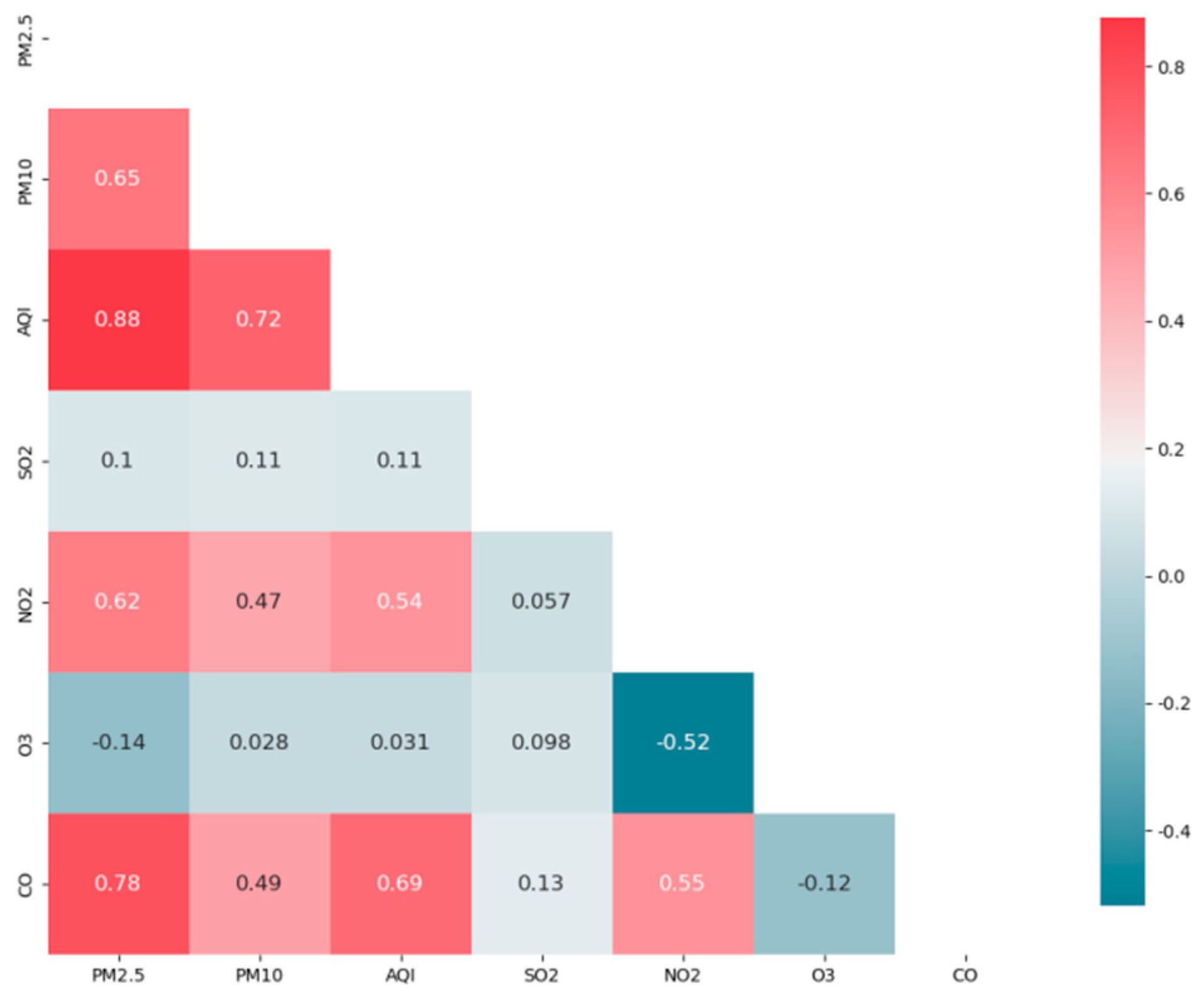
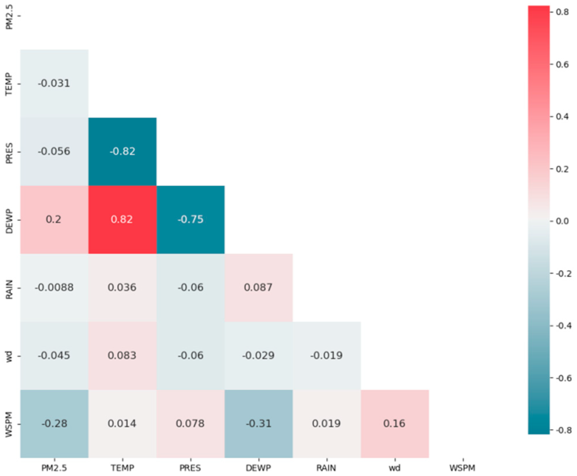
• The spatial and temporal correlation of historical air quality and meteorological data from 35 monitoring stations in Beijing is fully considered and effectively extracted. Through Spearman correlation analysis and access to atmospheric knowledge, AQI, CO, NO₂, and PM₁₀ concentrations from the air quality data and Dew Point Temperature (DEWP) and Wind Speed from the meteorological data are selected to better improve the prediction efficiency by almost 27%.
• The predictor including Spearman correlation analysis and Informer model are designed to predict the hourly PM_2.5 concentration in Beijing. Informer receives the extra-long history input data and generates the predicted output directly in one step, avoiding accumulation of errors due to step-by-step prediction. The predictor effectively solves the problem of decreasing the accuracy of long time series in existing prediction methods.
• As a result of performance evaluation, the proposed model has a good performance in predicting the hourly PM_2.5 concentration in future 7 days, 14 days, and one month. Compared with the existing methods, it has vastly improved at least 19–35%, and it has vital practical application significance for the government’s governance policies and people’s travel plans.

2. Materials and Methods

2.1. Data Collection

In the study of this paper, Beijing hourly air quality data and meteorological data from 1 January 2019 to 31 October 2022 are selected. The air quality data are obtained from Beijing Ecological Environment Monitoring Center (http://www.bjmemc.com.cn (accessed on 10 November 2022)), and the meteorological data are obtained from the National Climate Data Center (https://www.ncei.noaa.gov (accessed on 10 November 2022)). The datasets include 35 monitoring stations in each administrative region of Beijing, as shown in Figure 1, and the specific data format is shown in

Table 1. Overall input variables for PM_2.5 concentration forecasting models.

Data Type	Variable	Range	Unit
Air Pollution	PM2.5	[1, 427]	μg/m3
	PM10	[0, 1016]	μg/m3
	O3	[1, 517]	μg/m3
	CO	[0.1, 9]	μg/m3
	NO2	[1, 262]	μg/m3
	SO2	[1, 280]	μg/m3
	AQI	[1, 500]	μg/m3
Meteorological	Air Temperature	[−19.4, 41.4]	°C
	Dew Point Temperature	[−35.2, 31.2]	°C
	Sea Level Pressure	[982.6, 1042.1]	hPa
	Wind Direction	[0, 360]	°
	Wind Speed Rate	[0.13, 2]	m/s

. Among the whole dataset, the data from January 2019 to December 2021 were used for training, and the data from January to October 2022 were used for testing.

2.2. Data Description and Preprocessing

In the processing of air quality and meteorological data from various monitoring stations in Beijing. The missing data were first filled by interpolation and the noisy data were removed by rolling averages in python. Then, the Spearman correlation coefficients were selected to analyze the correlation between PM_2.5 concentration and both air quality and meteorological input data in terms of variables. After selecting the factors with high correlation, the air quality factors with weak correlation are removed and the meteorological data are integrated into the model for training, which not only improves the efficiency of the model but also improves the accuracy of the prediction. When training the model, the input is the historical PM_2.5 concentration and six variables with the strongest correlation among air quality and meteorological data, totaling seven variables, and the output is the PM_2.5 concentration in different time series in the future. The input data are transformed into the same range by normalization, thus eliminating the influence of two dimensions and variable changes and improving the convergence speed of the model.

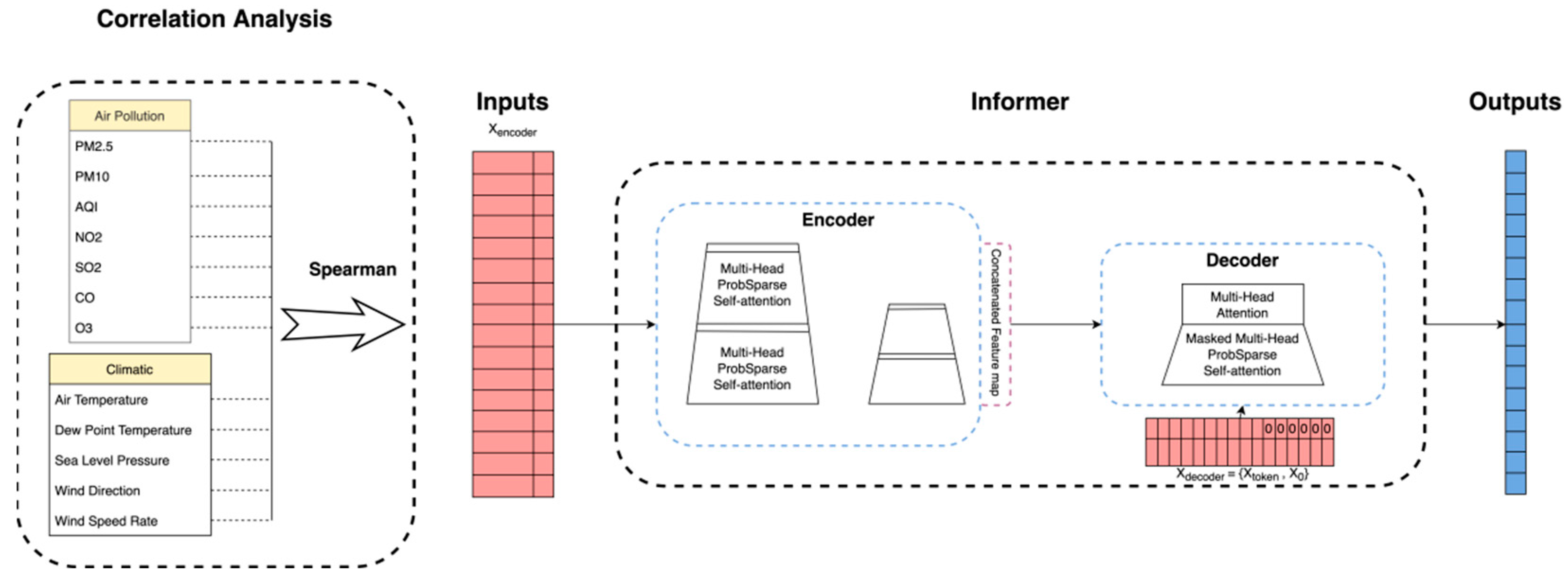
2.3. Correlation Analysis

Spearman rank correlation is a measure of the strength of the monotonic relationship between two continuous variables, taking values in the range [−1, 1]. The coefficient is a common method of measuring the statistical significance of trends in time series. Rank correlation is a statistic obtained by ranking the sample values of two variables in the order of their size and replacing the actual data with the rank of the sample values of each element. The variables x and y are ranked from smallest to largest, and are expressed in terms of rank r_x and r_y. When sorting, the phenomenon that the data are equal and thus have the same rank is called tie, in which case the average rank is taken as the rank of each data. The Spearman correlation coefficient, expressed as ρ_s, can be calculated by the following equation.

$${\rho }_s=1-\frac{6{\sum }^{ }{\left(r_{xi}-r_{yi}\right)}^2}{n\left(n^2-1\right)}$$

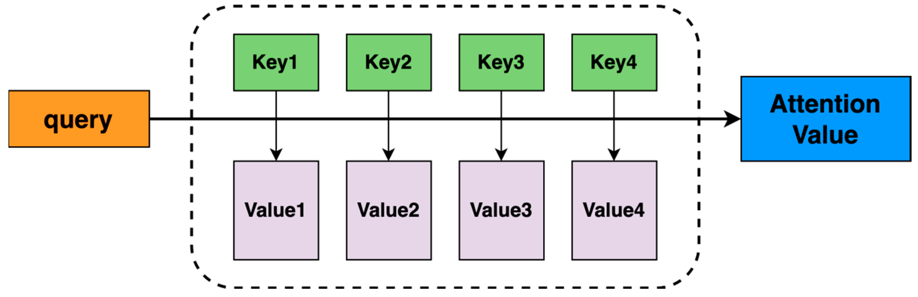
2.4. Attention Mechanism

The attention mechanism is similar to the human attention mechanism. By quickly scanning the global text, humans can quickly process it in the brain to obtain the area that needs to be focused, which is generally called the attention focus. Then, humans will devote more attention to this area to obtain more detailed information about the target that needs to be focused on while ignoring other useless information. The existence of this mechanism has greatly improved the means for humans to filter out high-value information from a large amount of information, and is a survival mechanism that has been developed by humans during long-term evolution.

The attention mechanism in deep learning is essentially similar to the human selectivity mechanism. The core goal is to select the information which is more critical to the current task goal from a large amount of information and focus on this important information, ignoring unimportant information. The larger the weight, the more it is focused on its corresponding value. Nowadays, the attention mechanism has been widely used in various types of deep learning tasks such as natural language processing, image recognition and speech recognition. It has become one of the core techniques in deep learning technology that deserves the most attention and in-depth understanding.

The calculation process of attention mechanism is shown in Figure 2. The attention mechanism is essentially a function that implements a mapping from query and a series of key-value pairs (key-value pairs) to the output, where query, key and value are all vectors. The output is obtained by weighted summation of values, and the weight corresponding to each value is obtained by query and key through a compatibility function. Depending on the actual situation, different functions and computational mechanisms can be introduced to calculate the similarity or correlation between query and a certain key and obtain attention value. The most common methods include: finding the dot product of the two vectors, the Cosine similarity of the two vectors, or finding the value by introducing additional neural networks.

2.5. Informer Model

The informer model [33] is an encoder-decoder structure, existing popular models are designed to encode the input representation X^t into the hidden state representation H^t, and the output representation Y^t, from the hidden state H^t = H^t₁,...... to decode. This prediction is designed as a stepwise process called “dynamic decoding”, in which the decoder computes a new hidden state H^t_k+1 based on the previous state H^t_k and other necessary outputs from the K step, and then predicts the K + 1 sequence Y^t_k+1.

The Informer has three improvements on the basis of transformer. Firstly, it proposes the ProbSparse self-attention mechanism with time complexity of O(LlogL), which reduces the computational complexity and space complexity of conventional self-attention. Secondly, the proposed self-attention distillation mechanism can shorten the length of the input sequence of each layer, which naturally reduces the computation and storage volume by using self-attention distillation technique to shorten the length of the input sequence of each layer and reduces the memory usage of J stacked layers. Thirdly, the proposed generative decoder mechanism gets the result in one step when predicting the sequence (also including the inference stage) instead of step-by-step, directly reducing the prediction time complexity from O(N) to O(1), changing the decoding method, and directly outputting the result in one step, effectively reducing the error.

The structure of the Informer model is shown in Figure 3. The encoder part is on the left side, which receives the extra-long input data and then replaces the traditional self-attention layer with the ProbSpare self-attention layer, which is unique to Informer. The self-attention distilling operation allows feature compression, and the encoder part improves the robustness of the algorithm by stacking the above two operations. The decoder part is on the right side, which receives a series of long sequence inputs and fills the predicted target positions with 0. Subsequently, the predicted output can be generated directly in one step after the masked attention layer.

2.6. Predictor Structure

As shown in Figure 3, the prediction model proposed in this paper consists of two parts: the variable extraction part of air quality and meteorological data and the Informer model part. In the extraction process of input variables, six variables with the strongest correlation between historical PM_2.5 concentrations and others are extracted by Spearman coefficient analysis to reduce irrelevant variables while fully considering spatial and temporal characteristics to improve the prediction accuracy. After the extraction, seven input variables are integrated into the Informer model and input into the encoder part. The ProbSpare self-attention mechanism is used to compress the features through the distilling operation further and enter the decoder layer. In the decoder layer, the prediction results can be output in one step, and finally obtain PM_2.5 concentration in different time series.

Compared with previously proposed models, our predictor adopts the ProbSparse self-attention mechanism and the self-attention distilling mechanism, which reduces computation and storage. Meanwhile, we use a generative decoding mechanism in the model to predict the output results in one step, effectively reducing the accumulation of errors caused by traditional methods of step-by-step prediction. Through a series of comparative experiments, we determined the reasonable model structure and hyperparameters, setting learning rate to 0.0001, epochs to 10, batch size to 32 for the 48 h and 7 days’ time series, and batch size to 16 for the 14 days and 30 days’ time series, using the early stopping method was used to overcome overfitting problems.

2.7. Evaluation Indicators

The PM_2.5 prediction performed in this study can be analogous to a regression modeling problem. Therefore, the combined performance of each model can be effectively evaluated by statistical-based regression analysis metrics. As classical statistical indicators, two evaluation indicators mean absolute error (MAE) and root mean square error (RMSE) are used in this paper to evaluate the performance of each model, which are calculated by the following equations.

$$\mathrm{RMSE}=\sqrt{\frac{1}{\mathrm{n}}{{\displaystyle \sum }}_{\mathrm{i}=1}^{\mathrm{n}}{\left({\mathrm{O}}_{\mathrm{i}}-{\mathrm{P}}_{\mathrm{i}}\right)}^2}$$

$$\mathrm{MAE}=\frac{1}{\mathrm{n}}{{\displaystyle \sum }}_{\mathrm{i}=1}^{\mathrm{n}}\left|{\mathrm{O}}_{\mathrm{i}}-{\mathrm{P}}_{\mathrm{i}}\right|$$

O_i, P_i and n denote observed values, predicted values and the number of evaluation samples, respectively. MAE and RMSE are evaluation metrics to evaluate the absolute error, and the smaller the values are, the better the model performances.

3. Results

3.1. Correlation Analysis of Variables

Table 2. Correlation analysis between PM_2.5 concentrations and other variables at all stations.

Input Variables				Output Variables
Air Pollution		Climatic		PM2.5(t + n)
AQI(t) 0.88	CO(t) 0.78	Air Temperature(t) −0.031	Wind Direction(t) −0.045
PM10(t) 0.65	NO2(t) 0.62	Dew Point Temperature(t) 0.2	Wind Speed(t) −0.28
O3(t) −0.14	SO2(t) 0.1	Sea Level Pressure(t) −0.056	Rain(t) −0.0088

shows the correlations between PM_2.5 concentrations and air quality and meteorological data in the selected data set. The correlation is also plotted in Figure 4 and Figure 5 by heat map. The correlation shows that among several types of air quality data, PM_2.5 concentration has a rather large positive correlation with AQI, CO, NO₂, and PM₁₀, a weak positive correlation with SO₂, and a negative correlation with O₃. This is because one of the major source of PM_2.5 is fossil fuels and vehicle emissions, and the combustion of coal and oil both produce CO, NO₂, and contribute to the production of air pollutants such as PM_2.5 and PM₁₀. The AQI is an indicator of the AQI and PM_2.5 is one of the indicators calculated by the AQI. As for O₃, unlike the source sources of PM_2.5, PM_2.5 is mainly caused by human activities, while O₃ is mainly from natural sources. The concentration of O₃ increases under strong light and high temperature, and some photochemical reactions may consume part of PM_2.5 and reduce its concentration due to the high concentration of O₃ [34].

In this study, the meteorological data from the monitoring stations are also integrated for improving the prediction accuracy of PM_2.5. In terms of traditional models and causes, air pollution can be affected by a variety of meteorological factors because meteorological conditions can affect the diffusion of pollutants. The correlation analysis revealed that PM_2.5 concentration has a strong positive correlation with Dew Point Temperature, which is a measure of air humidity, and when air humidity increases, it contributes to the formation of fine particulate matter and more pollutants that are not easily diffused exist in the air [35]. PM_2.5 concentration has a negative correlation with wind speed because high wind speed is conducive to the diffusion of pollutants to the upper atmosphere, resulting in lower PM_2.5 concentration. Except for that, the correlation between PM_2.5 concentration, sea level pressure, air temperature, and rainfall is relatively weak.

Through the above correlation analysis and access to atmospheric knowledge, AQI, CO, NO₂, and PM₁₀ concentrations are selected from the air quality data, and Dew Point Temperature (DEWP) and wind speed are incorporated from the meteorological data to better improve the prediction efficiency and accuracy.

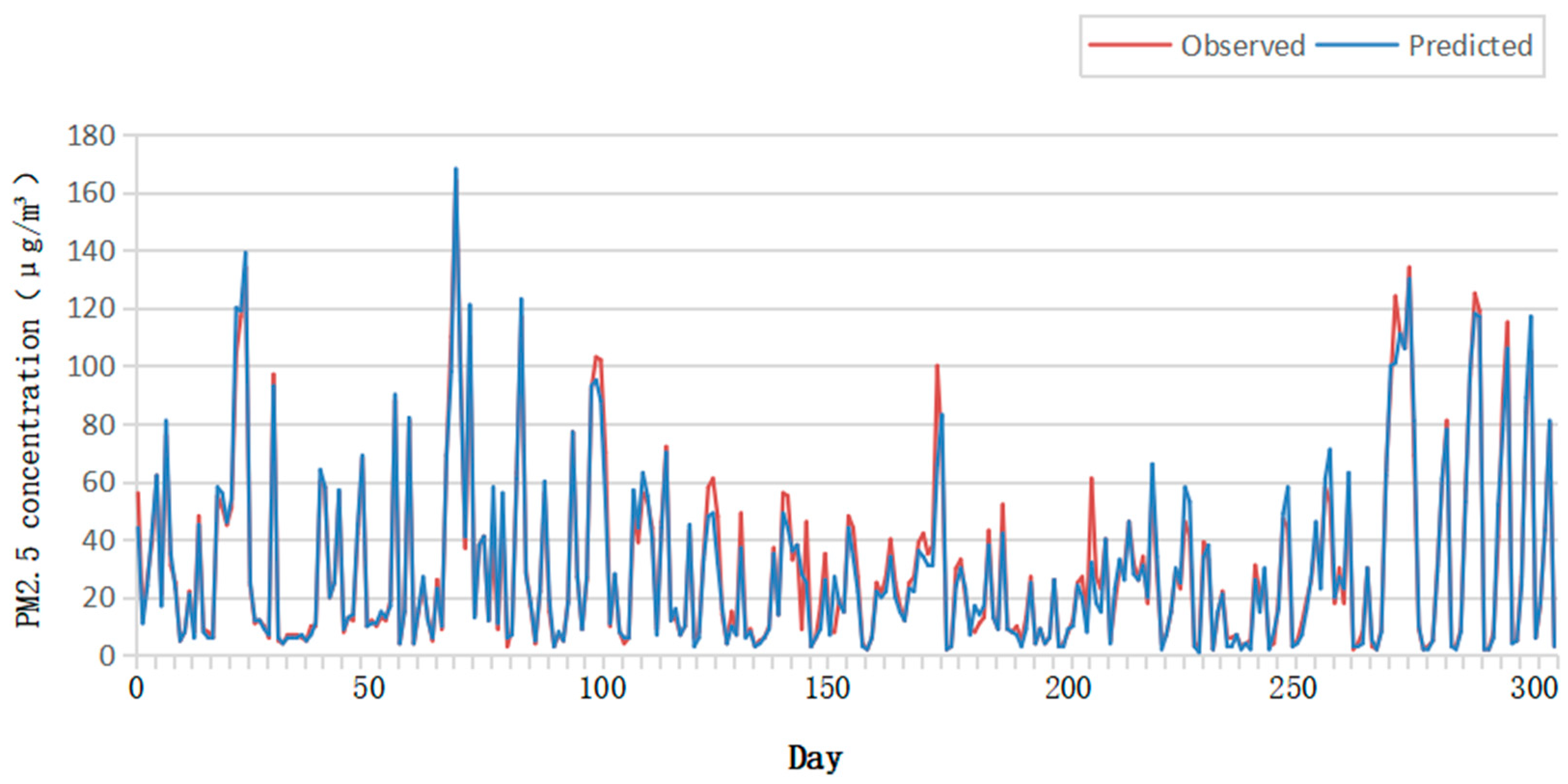
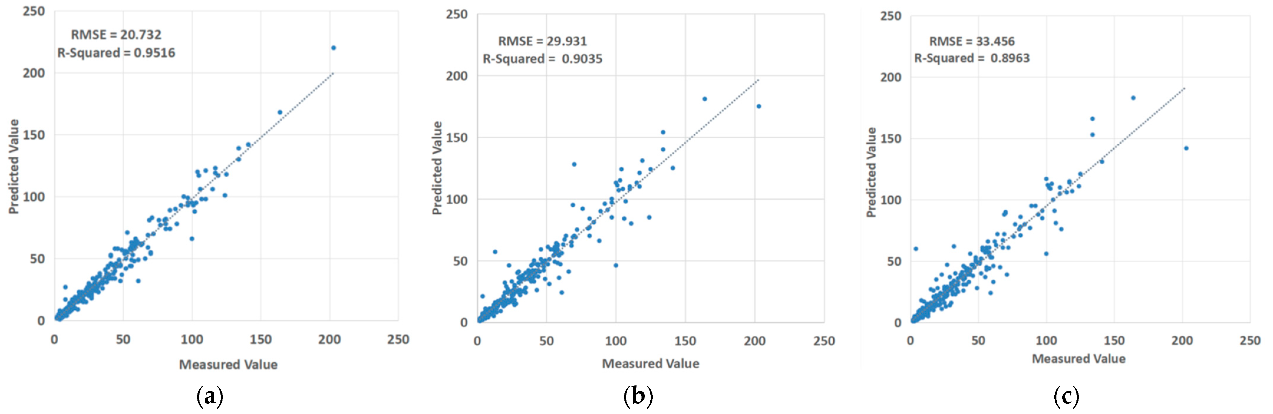
3.2. Prediction Performance Validation

The proposed model has used the data from January 2019 to December 2021 for training and the data from January to October 2022 for testing. The performance of predicting PM_2.5 concentrations for the next 7 days are shown in Figure 6.

In Figure 6, the red and blue lines represent the observed and predicted values of PM_2.5, respectively. In terms of the follow-through of the predicted values to the observed values, the model in this paper shows accurate prediction performance over the entire prediction range. This indicates that the proposed model exhibits nonlinear patterns such as seasonality and performs well, even when the air quality changes abruptly.

In

Table 3. The comparison of LSTM, Attention-LSTM and our predictor in prediction performance.

Network	48 h		7 Days		14 Days		30 Days
	RMSE	MAE	RMSE	MAE	RMSE	MAE	RMSE	MAE
LSTM	15.694	13.124	23.238	18.549	33.456	22.621	46.812	29.413
Attention-LSTM	14.283	12.437	21.419	15.205	29.931	20.468	44.093	25.123
Our predictor	11.276	9.213	17.498	13.503	20.732	14.693	24.211	18.867

, our predictor is compared with other models in terms of RMSE and MAE evaluation metrics, as well as different prediction time series. In Figure 7, scatter plots are plotted comparing the performance of each model when forecasting the future 14 days’ time series. It can be seen that our predictor shows good advantages not only for short time series, but also for long time series.

3.3. Effects of Different Forecast Time on Model Performance

In this study, different prediction time series are used as variables for forecasting, and the LSTM model, the attention-LSTM model are compared with our predictor to examine the prediction performance in long time series. The future 48 h, 7 days, 14 days, and 30 days four different time series are selected. The evaluated performance of the model gradually decreases as the forecast length increases, and both RMSE and MAE gradually increase.

In the process of predicting the hourly PM_2.5 concentration in the next 48 h, our predictor model is closer to the errors of the LSTM and attention-LSTM models, but still shows relatively good results. In the process of predicting hourly PM_2.5 concentrations during the future 7 days, 14 days, and 1 month, the LSTM and attention-LSTM model errors increase rapidly in RMSE and MAE due to the accumulation of errors in stepwise prediction, while the model used in this paper has a slower increase in RMSE and MAE error values as the prediction period increases. Our predictor model shows superior performance in longer time series forecasting.

3.4. Comparison of Informer with Other Prediction Methods

Currently, many researchers have proposed various advanced models and analyses in the field of PM_2.5 concentration prediction, which have achieved remarkable results. The model proposed in this paper is compared with the traditional model, which effectively demonstrates the improved effect for long time series prediction. The analysis is derived from the performance assessment comparison in Table 3 and Figure 7 as follows.

• Through comparison, it can be found that more advanced models will obtain better PM_2.5 prediction results with the same prediction time. For example, the introduction of the attention mechanism will reduce the error to a certain extent and optimize the performance of the LSTM, which shows that advanced models can effectively integrate the advantages of each algorithm component from multiple aspects and effectively improve the overall prediction accuracy of the prediction model. It fully demonstrates that the approach of feature extraction and integrated learning is important for optimizing the overall prediction performance of the model.
• The model proposed in this paper can achieve better prediction results than LSTM and attention-LSTM models for the tested prediction time series, which shows that the model proposed in this paper performs very well in the prediction of long time series and makes up for the shortcomings of the existing methods in the prediction of long time series. The proposed model has good practical application prospects in the PM_2.5 concentration prediction problem. It proves the feasibility of using this method for PM_2.5 concentration prediction, and it can also be implemented for the prediction of other air pollution indicators, such as AQI, CO, NO₂, etc.

4. Discussion

4.1. Concentration Fluctuation Pattern of PM_2.5

In the study, the actual PM_2.5 concentration values from January 2019 to October 2022 are presented through the time dimension and the PM_2.5 concentration fluctuation pattern is summarized based on Figure 8.

When the data are presented on an annual cycle, it can be found that PM_2.5 concentrations vary significantly in different seasons. PM_2.5 concentrations are lower in summer and autumn, and higher in spring and winter. There is a steady upward tendency in the low PM_2.5 concentration of summer and autumn. This is due to the higher surface temperature during summer, which heats up the ground air, intensifies convection, and increases precipitation. This makes it more inclined to vertical diffusion and deposition, resulting in lower PM_2.5 concentrations. In autumn when the weather is generally smoother without rapid and drastic weather changes, while biomass burning occurs frequently, PM_2.5 concentrations gradually tend to increase [36,37].

Higher PM_2.5 concentrations during the year occur mainly in winter and spring from November to March, with the highest peak emerging in December, but with large variability, indicating the transient and concentrated nature of pollution outbreaks. Compared with summer and autumn, the weather in winter and spring is dry with little rain. Dust storms from the arid northwestern region contribute to some extent to the elevated PM_2.5 concentrations. Human behavior also plays a prominent role in affecting PM_2.5 concentration anomalies. Beijing and the surrounding areas have one of the highest concentrations of large-scale industry in China which consumes a great deal of fossil fuel and produces a large amount of industrial emissions. During the autumn and winter of the heating period, coal smoke pollutants caused by industrial boilers and heating boilers increased significantly. Although the atmosphere is stable, the frequency and intensity of inversion is high, and it is difficult for pollutants to disperse, resulting in higher PM_2.5 concentrations near the ground end. Meanwhile, increased passenger traffic and the use of fireworks during the Chinese New Year also result in the rapid increase in PM_2.5 concentrations [38,39].

Meanwhile, according to the three-year fluctuation trend, while the amount of blue sky in Beijing increased greatly, the number of heavy pollution days reduced significantly, as did their frequency and length, and heavy pollution was almost eradicated in the summer and fall. PM_2.5 concentration is currently declining steadily. Beijing has shut down some of its heavily polluting industries in recent years, increased greenery on a large scale, and planted protective forests to mitigate dust storms. In addition, the rapid development of new energy vehicles has reduced vehicle emissions, all of which have contributed to the reduction in PM_2.5 concentrations.

4.2. Model Selection

The prediction model used in this paper is a deep learning model, however the traditional numerical models such as WRF-Chem and CMAQ can be another useful tool for predicting PM_2.5 concentrations. Compared to numerical models, we believe that the proposed deep learning model is more timely, simplified, and generic. The input data for deep learning models, including air quality data and meteorological data, can be collected and updated from publicly available databases in a timely and convenient manner. In contrast, input data for some numerical models, such as emission source lists, are often difficult for NGOs to access. In the future, the comparison of the advantages and disadvantages of deep learning and numerical models merits further research.

In this paper, we focused on and proposed an optimized PM_2.5 concentration predictor model. The predictor can be further applied by developing web applications to trace PM_2.5 concentration with the touch of fingertip or the click of a mouse. All such works are options we can continue to work on in the future.

5. Conclusions

In this paper, we proposed the spatiotemporal predictor which includes the Spearman correlation analysis and Informer model to predict lone time series hourly PM_2.5 concentration in Beijing. At first, we conducted the correlation analysis of historical air quality and meteorological data from 35 environmental monitoring stations distributed in all districts of Beijing. The spatial and temporal correlations associated with the target parameter PM_2.5 were fully considered and effectively extracted. We selected AQI, CO, NO₂, PM₁₀ concentrations, Dew Point Temperature (DEWP), and wind speed, six variables for input into the model by Spearman correlation analysis for training to predict hourly PM_2.5 concentrations in Beijing at different time series in the future. Compared with LSTM and attention-LSTM models through statistical indicators RMSE and MAE, it is fully demonstrated that the model constructed in this paper has shown a greater advantage in the PM_2.5 concentration prediction problem especially for the longer time series, with at least 21%, 19%, 28%, and 35% improvement in accuracy in four prediction time series: 48 h, 7 days, 14 days, and 30 days. The proposed model shows a higher accuracy and stability.

There are still some limitations in this paper, such as not dealing well with the spatial effects of distance, interaction relations, and weights between monitoring stations, and the accuracy is not greatly improved in short time series prediction. In light of this, a better combination of traditional methods and deep learning methods can be constructed. In the future, researchers could further explore how to better optimize the model structure to improve the accuracy rate.

References

1. Riojas-Rodríguez, H.; Romieu, I.; Hernández-Ávila, M. Air pollution. In Occupational and Environmental Health; Oxford University Press: Oxford, UK, 2017; pp. 345–364. ISBN 9780190662677. [Google Scholar]
2. WHO. Health Aspects of Air Pollution with Particulate Matter, Ozone and Nitrogen Dioxide. Tech. Rep. WHO 2003, 7–9. [Google Scholar]
3. Xing, Y.F.; Xu, Y.H.; Shi, M.H.; Lian, Y.X. The impact of PM 2.5 on the human respiratory system. J. Thorac. 2016, 8, 69–74. [Google Scholar] [CrossRef]
4. Kampa, M.; Castanas, E. Human health effects of air pollution. Environ. Pollut. 2008, 151, 362–367. [Google Scholar] [PubMed]
5. WHO. Ambient air pollution: A global assessment of exposure and burden of disease. In WHO Library Cataloguing-in-Publication Data; WHO: Geneva, Switzerland, 2016. [Google Scholar]
6. Tian, Y.; Jiang, Y.; Liu, Q.; Xu, D.; Zhao, S.; He, L.; Liu, H.; Xu, H. Temporal and spatial trends in air quality in Beijing. Landsc. Urban Plann. 2019, 185, 35–43. [Google Scholar] [CrossRef]
7. Wang, G.; Xue, J.; Zhang, J.; Centre, N.M. Analysis of spatial-temporal distribution characteristics and main cause of air pollution in Beijing-Tianjin-Hebei region in 2014. Meteorol. Environ. 2016, 39, 34–42. [Google Scholar]
8. Tang, H.; Chen, W.; Zhao, H. Diurnal, weekly and monthly spatial variations of air pollutants and air quality of Beijing. Atmos. Environ. 2015, 119, 21–34. [Google Scholar]
9. Xu, W.; Tian, Y.; Xiao, Y.; Jiang, W.; Tian, L.; Liu, J. Study on the spatial distribution characteristics and the drivers of AQI in North China. Huanjing Kexue Xuebao/Acta Sci. Circumstantiae 2017, 37, 3085–3096. [Google Scholar]
10. Baklanov, A.; Mestayer, P.G.; Clappier, A.; Zilitinkevich, S.; Joffre, S.; Mahura, A.; Nielsen, N.W. Towards improving the simulation of meteorological fields in urban areas through updated/advanced surface fluxes description. Atmos. Chem. Phys. 2008, 8, 523–543. [Google Scholar] [CrossRef]
11. Kim, Y.; Fu, J.S.; Miller, T.L. Improving ozone modeling in complex terrain at afine grid resolution:part I-examinationof analysis nudging andall PBL schemes associated with LSMs in meteorological model. Atmos. Environ. 2010, 44, 523–532. [Google Scholar] [CrossRef]
12. Woody, M.C.; Wong, H.W.; West, J.J.; Arunachalama, S. Multiscale predictions of aviation-attributable PM2.5 for U.S. airports modeled using CMAQ withplume-in-grid and an aircraft-specific 1-D emission model. Atmos. Environ. 2016, 147, 384–394. [Google Scholar] [CrossRef]
13. Bray, C.D.; Battye, W.; Aneja, V.P.; Tong, D.; Lee, P.; Tang, Y.; Nowak, J.B. Evaluating ammonia (NH 3) predictions in the NOAA National Air Quality Forecast Capability (NAQFC) using in-situ aircraft and satellite measurements from the CalNex 2010 campaign. Atmos. Environ. 2017, 163, 65–76. [Google Scholar] [CrossRef]
14. Zhou, G.; Xu, J.; Xie, Y.; Chang, L.; Gao, W.; Gu, Y.; Zhou, J. Numerical air quality forecasting over eastern China: An operational application of WRF-Chem. Atmos. Environ. 2017, 153, 94–108. [Google Scholar] [CrossRef]
15. Carlo, P.D.; Pitari, G.; Mancini, E.; Gentile, S.; Pichelli, E.; Visconti, G. Evolution of surface ozone in central Italy based on observations and statistical model. J. Geophys. Res. 2007, 112. [Google Scholar] [CrossRef]
16. Castellano, M.; Franco, A.; Cartelle, D.; Febrero, M.; Roca, E. Identification of NOx and ozone episodes and estimation of ozone by statistical analysis. Water Air Soil Pollut. 2009, 198, 95–110. [Google Scholar] [CrossRef]
17. Gennaro, G.; Trizioa, L.; Gilioa, A.D.; Pey, J.; Pérez, N.; Cusack, M.; Alastuey, A.; Querol, X. Neural network model for the prediction of PM 10 daily concentrations in two sites in the Western Mediterranean. Sci. Total Environ. 2013, 463, 875–883. [Google Scholar] [CrossRef] [PubMed]
18. Donnelly, A.; Misstear, B.; Broderick, B. Real time air quality forecasting using integrated parametric and non-parametric regression techniques. Atmos. Environ. 2015, 103, 53–65. [Google Scholar] [CrossRef]
19. Yuan, X.; Chen, C.; Lei, X.; Yuan, Y.; Muhammad Adnan, R. Monthly runoff forecasting based on LSTM–ALO model. Stoch. Environ. Res. Risk Assess. 2018, 32, 2199–2212. [Google Scholar] [CrossRef]
20. Adnan, R.M.; Mostafa, R.R.; Elbeltagi, A.; Yaseen, Z.M.; Shahid, S.; Kisi, O. Development of new machine learning model for streamflow prediction: Case studies in Pakistan. Stoch. Environ. Res. Risk Assess. 2022, 36, 999–1033. [Google Scholar]
21. Adnan, R.M.; Mostafa, R.R.; Islam, A.R.M.T.; Kisi, O.; Kuriqi, A.; Heddam, S. Estimating reference evapotranspiration using hybrid adaptive fuzzy inferencing coupled with heuristic algorithms. Comput. Electron. Agric. 2021, 191, 106541. [Google Scholar]
22. Ikram, R.M.A.; Dai, H.-L.; Ewees, A.A.; Shiri, J.; Kisi, O.; Zounemat-Kermani, M. Application of improved version of multi verse optimizer algorithm for modeling solar radiation. Energy Rep. 2022, 8, 12063–12080. [Google Scholar] [CrossRef]
23. Adnan, R.M.; Kisi, O.; Mostafa, R.R.; Ahmed, A.N.; El-Shafie, A. The potential of a novel support vector machine trained with modified mayfly optimization algorithm for streamflow prediction. Hydrol. Sci. J. 2022, 67, 161–174. [Google Scholar] [CrossRef]
24. Ikram, R.M.A.; Ewees, A.A.; Parmar, K.S.; Yaseen, Z.M.; Shahid, S.; Kisi, O. The viability of extended marine predators algorithm-based artificial neural networks for streamflow prediction. Appl. Soft Comput. 2022, 131, 109739. [Google Scholar] [CrossRef]
25. Ikram, R.M.A.; Dai, H.-L.; Chargari, M.M.; Al-Bahrani, M.; Mamlooki, M. Prediction of the FRP reinforced concrete beam shear capacity by using ELM-CRFOA. Measurement 2022, 205, 112230. [Google Scholar] [CrossRef]
26. Pak, U.; Kim, C.; Ryu, U.; Sok, K.; Pak, S. A hybrid model based on convolutional neural networks and long short-term memory for ozone concentration prediction. Air Qual. Atmos. Health 2018, 11, 883–895. [Google Scholar] [CrossRef]
27. Ong, B.T.; Sugiura, K.; Zettsu, K. Dynamic pre-training of deep recurrent neural networks for predicting environmental monitoring data. In Proceedings of the IEEE International Conference on Big Data, Washington, DC, USA, 27–30 October 2014; Volume 16, pp. 760–765. [Google Scholar] [CrossRef]
28. Biancofiore, F.; Busilacchio, M.; Verdecchia, M.; Tomassetti, B.; Aruffo, E.; Bianco, S.; Di Tommaso, S.; Colangeli, C.; Rosatelli, G.; Di Carlo, P. Recursive neural network model for analysis and forecast of PM10 and PM2.5. Atmos. Pollut. 2017, 8, 652–659. [Google Scholar] [CrossRef]
29. Li, X.; Peng, L.; Yao, X.; Cui, S.; Hu, Y.; You, C.; Chi, T. Long short-term memory neural network for air pollutant concentration predictions: Method development and evaluation. Environ. Pollut. 2017, 231, 997–1004. [Google Scholar] [CrossRef] [PubMed]
30. Soh, P.W.; Chang, J.W.; Huang, J.W. Adaptive deep learning-based air quality prediction model using the most relevant spatial-temporal relations. IEEE Access. 2018, 6, 38186–38199. [Google Scholar] [CrossRef]
31. Liao, Q.; Zhu, M.; Wu, L.; Pan, X.; Tang, X.; Wang, Z. Deep learning for air quality forecasts: A review. Curr. Pollut. 2020, 6, 399–409. [Google Scholar] [CrossRef]
32. Liu, H.; Yan, G.; Duan, Z.; Chen, C. Intelligent modeling strategies for forecasting air quality time series: A review. Appl. Soft Comput. 2021, 102, 106957. [Google Scholar]
33. Zhou, H.; Zhang, S.; Peng, J.; Zhang, S.; Li, J.; Xiong, H.; Zhang, W. Informer: Beyond Efficient Transformer for Long Sequence Time-Series Forecasting. In Proceedings of the AAAI Conference on Artificial Intelligence; AAAI Press: Palo Alto, CA, USA, 2021; Volume 35, pp. 11106–11115. [Google Scholar] [CrossRef]
34. Luo, Y.P.; Liu, M.J.; Gan, J.; Zhou, X.T.; Jiang, M.; Yang, R.B. Correlation study on PM2.5 and O3 mass concentrations in ambient air by taking urban cluster of Changsha, Zhuzhou and Xiangtan as an example. J. Saf. Environ. 2015, 15, 313–317. [Google Scholar]
35. Zhang, Z.; Zhang, X.; Gong, D.; Quan, W.; Zhao, X.; Ma, Z.; Kim, S.J. Evolution of surface O3 and PM2.5 concentrations and their relationships with meteorological conditions over the last decade in Beijing. Atmos. Environ. 2015, 108, 67–75. [Google Scholar] [CrossRef]
36. Cheng, Y.; Engling, G.; He, K.B.; Duan, F.K.; Ma, Y.L.; Du, Z.Y.; Liu, J.M.; Zheng, M.; Weber, R.J. Biomass burning contribution to Beijing aerosol. Atmos. Chem. Phys. 2013, 13, 7765–7781. [Google Scholar] [CrossRef]
37. Cui, J.; Lang, J.; Chen, T.; Mao, S.; Cheng, S.; Wang, Z.; Cheng, N. A framework for investigating the air quality variation characteristics based on the monitoring data: Case study for Beijing during 2013–2016. J. Environ. 2019, 81, 225–237. [Google Scholar] [CrossRef] [PubMed]
38. Jiang, Q.; Sun, Y.L.; Wang, Z.; Yin, Y. Aerosol composition and sources during the Chinese Spring Festival: Fireworks, secondary aerosol, and holiday effects. Atmos. Chem. Phys. 2015, 15, 20617–20646. [Google Scholar]
39. Zhang, Y.; Sun, Y.; Du, W.; Wang, Q.; Chen, C.; Han, T.; Lin, J.; Zhao, J.; Xu, W.; Gao, J.; et al. Response of aerosol composition to different emission scenarios in Beijing, China. Sci. Total Environ. 2016, 571, 902–908. [Google Scholar]
Figure 1. The distribution of air quality monitoring stations in China.
Atmosphere 14 00340 g001
Figure 2. The calculation process of attention mechanism.
Atmosphere 14 00340 g002
Figure 3. The structure of our predictor model.
Atmosphere 14 00340 g003
Figure 4. Heat map of correlation between PM2.5 concentration and air quality variables.
Atmosphere 14 00340 g004
Figure 5. Heat map of correlation between PM2.5 concentration and climatic variables.
Atmosphere 14 00340 g005
Figure 6. The comparison of observed and predicted values from January to October 2022.
Atmosphere 14 00340 g006
Figure 7. The performance of three models in predicting future 14 days from January to October 2022. (a) LSTM, (b) attention-LSTM, (c) our predictor.
Atmosphere 14 00340 g007
Figure 8. The trends of PM2.5 concentration from January 2019 to October 2022.
Atmosphere 14 00340 g008