
Size Distribution of Chemical Components of Particulate Matter in Lhasa
Abstract
:1. Introduction
2. Material and Methods
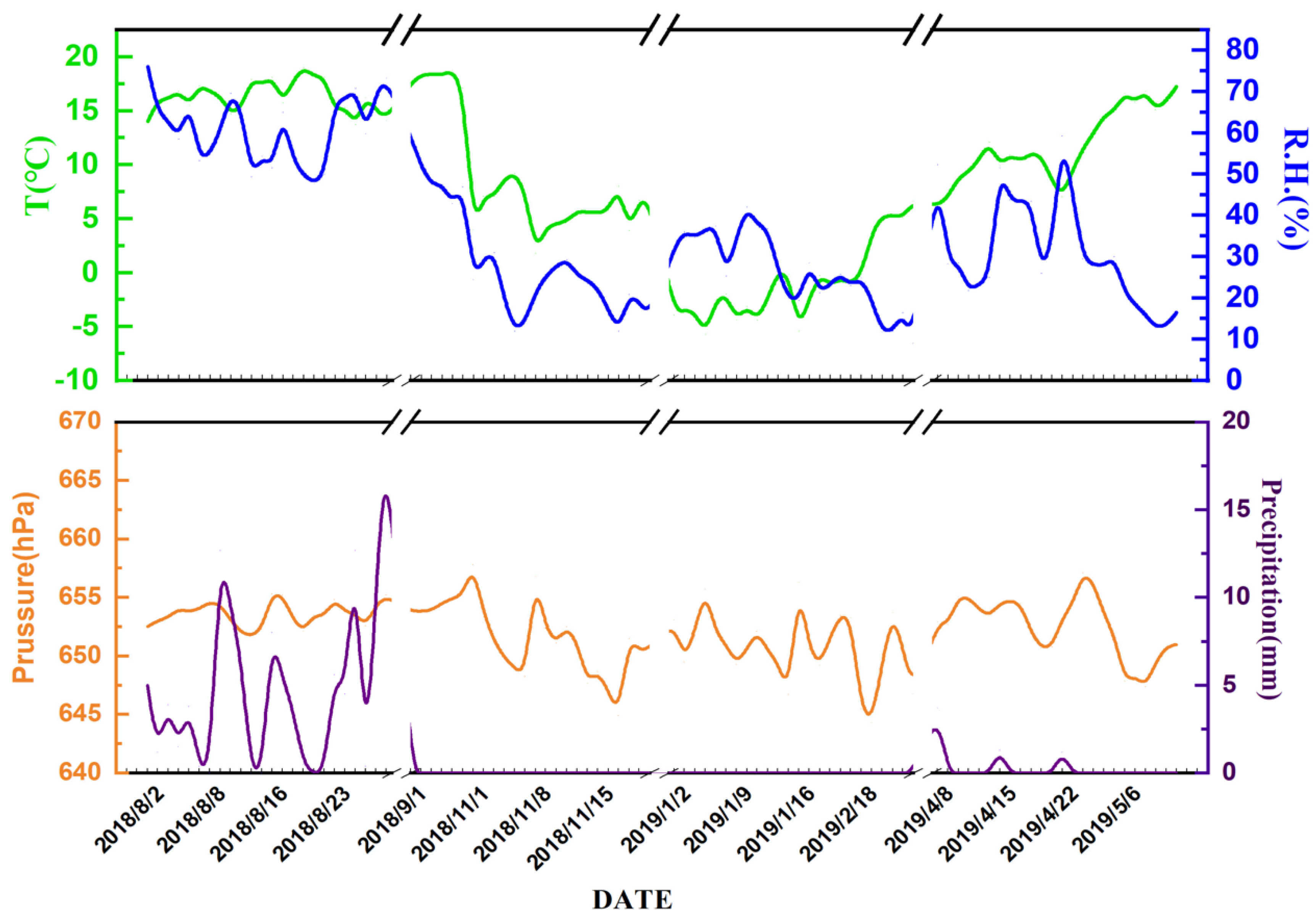
2.1. Sampling Sites and Samples Collection
2.2. Analytical Methods
2.3. Principal Component Analysis
3. Results and Discussion
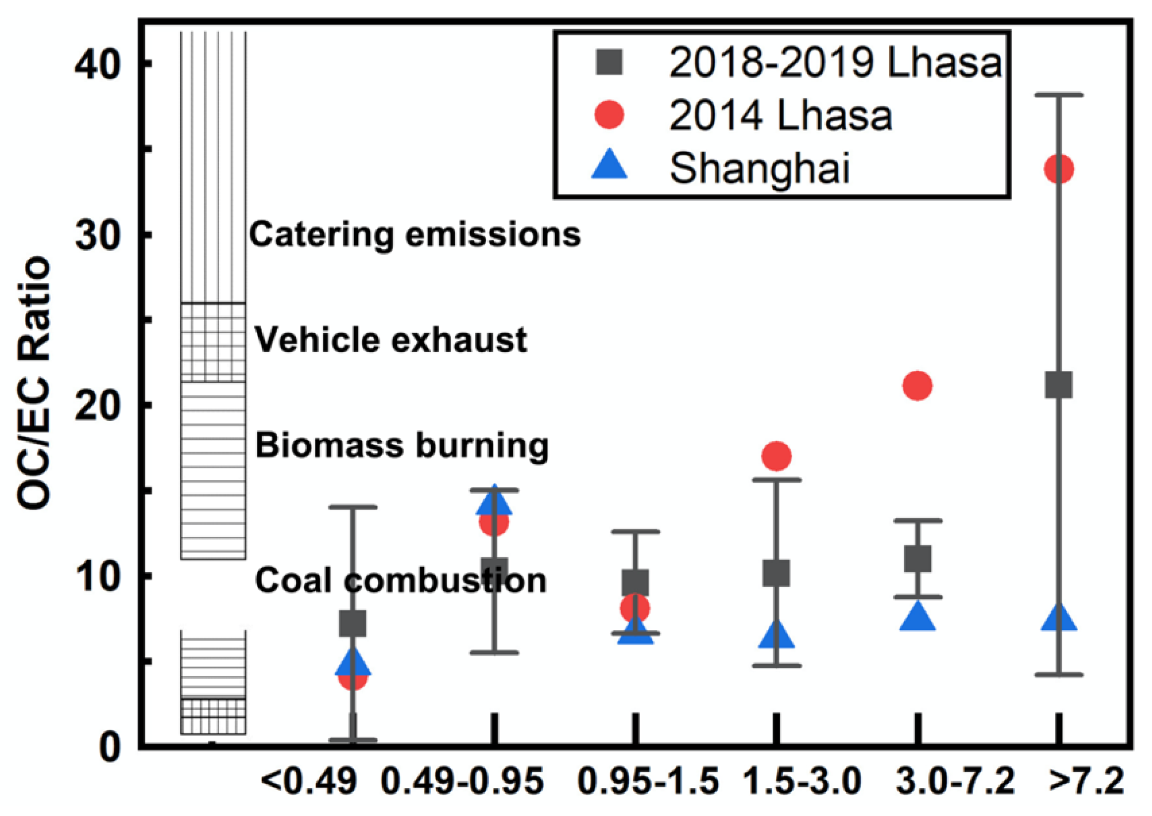
3.1. PM and Carbon Fractions
3.1.1. Size Distribution and Temporal Variations
3.1.2. Secondary Aerosol Analysis
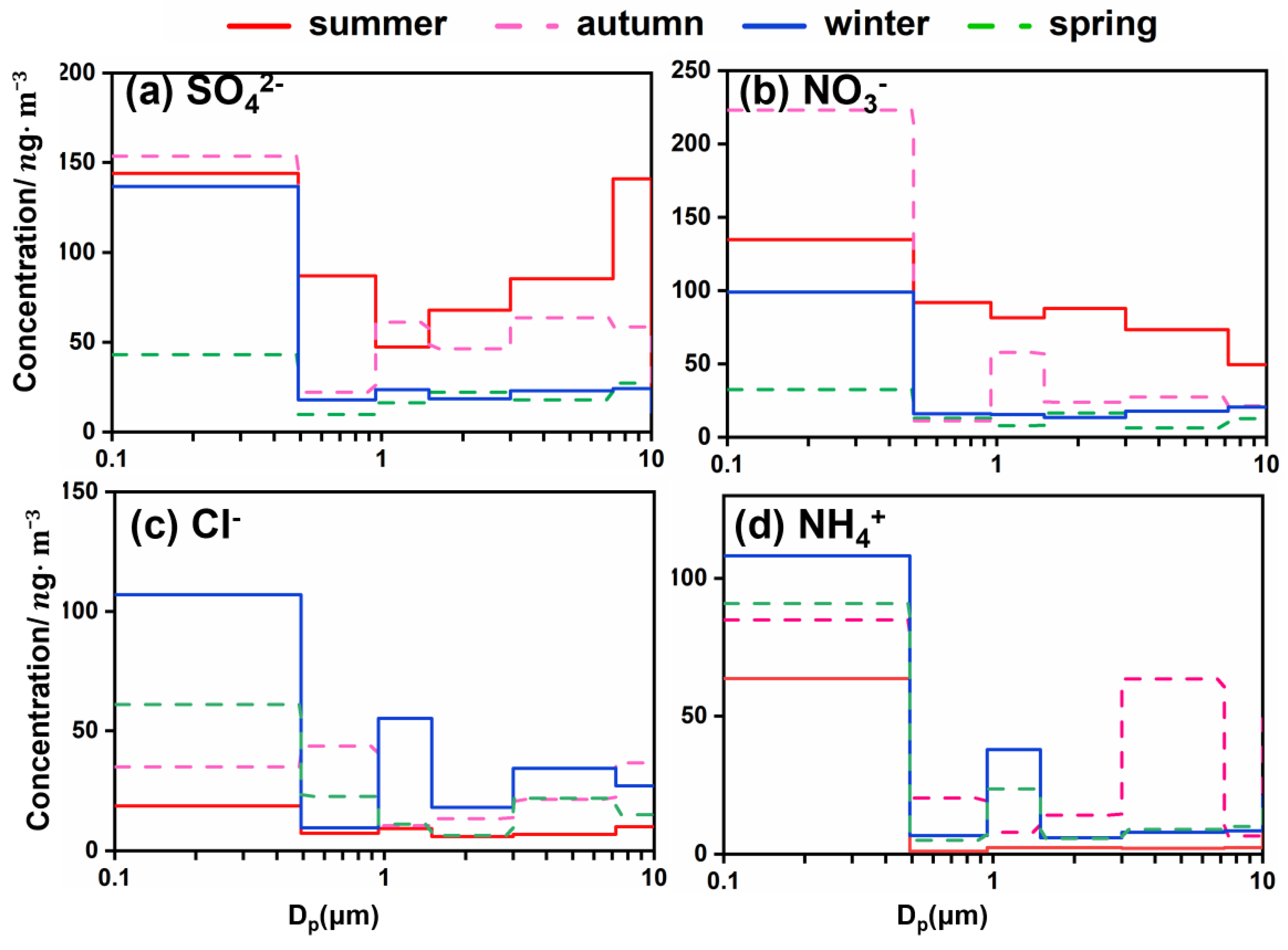
3.2. Water-Soluble Ions
3.2.1. Size Distribution and Temporal Variations
3.2.2. [NO3−]–[SO42−]
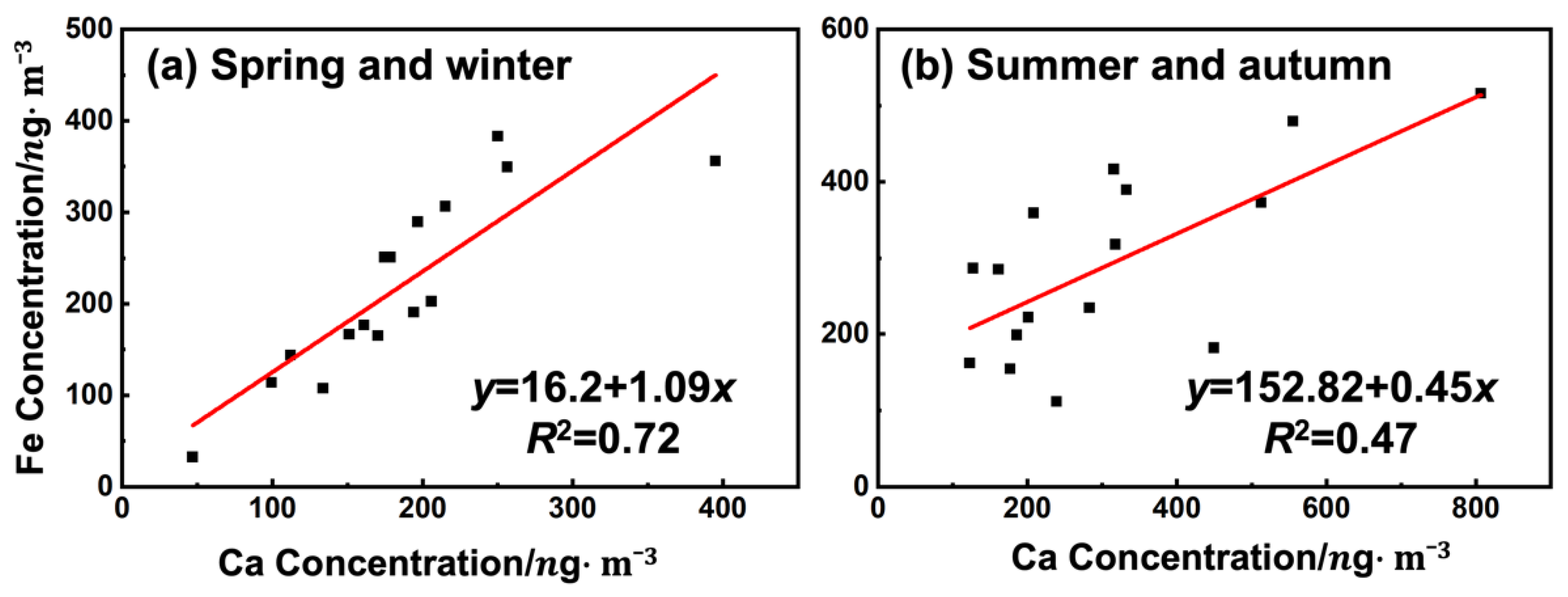
3.3. Trace Elements
3.3.1. Trace Elements in Total Suspended Dust (TSP)
3.3.2. Size Distribution and Temporal Variations
3.4. Source Apportionment of PM in Lhasa
4. Conclusions
Author Contributions
Funding
Informed Consent Statement
Data Availability Statement
Conflicts of Interest
Appendix A


| Location | Periods | Mg | Al | K | Ca | Ti | V | Cr | Mn | Ni | Cu | Zn | Pb | Fe | Reference |
|---|---|---|---|---|---|---|---|---|---|---|---|---|---|---|---|
| (ng·m−3) | |||||||||||||||
| Lhasa | 2018–2019 | 122.8 | 1057 | 425.1 | 551.5 | 40.02 | 3.278 | 1.047 | 8.66 | 0.02 | 125.73 | 5.19 | 4.08 | 682 | |
| Chifeng | 2016–2017 | 168.9 | 547.3 | 1012 | 454.3 | 26.9 | 1.8 | 2.4 | 16.6 | 1.2 | 16.5 | 83.7 | 51 | 390 | [79] |
| Chengdu | 2014–2015 | --- | 281 | 720 | 240 | 32.5 | 1.9 | 5.6 | 33.8 | 2.1 | 18.7 | 238 | 55.4 | 456 | [80] |
| Beijing | 2009–2010 | 600 | 970 | 1730 | 2420 | 40 | 3.3 | 19.9 | 72.6 | 7.5 | 44.3 | 113 | 50.4 | 586 | |
| Tianjin | 700 | 1170 | 2150 | 3280 | 40 | 4.9 | 13.4 | 102 | 7.3 | 138 | 324 | 142 | 1490 | [65] | |
| Nanjing | 2013–2014 | 209 | 705 | --- | 1520 | --- | 9.88 | 13.2 | --- | 9.3 | 24.7 | 746 | 220 | 2020 | |
| Shanghai | 298 | 922 | --- | 1930 | --- | 16.5 | 16.9 | --- | 14.9 | 24.2 | 677 | 298 | 1840 | [81] |
References
- Chow, J.C.; Watson, J.G.; Lowenthal, D.H.; Magliano, K.L. Size-Resolved Aerosol Chemical Concentrations at Rural and Urban Sites in Central California, USA. Atmos. Res. 2008, 90, 243–252. [Google Scholar] [CrossRef]
- Pan, Y.; Tian, S.; Li, X.; Sun, Y.; Li, Y.; Wentworth, G.R.; Wang, Y. Trace Elements in Particulate Matter from Metropolitan Regions of Northern China: Sources, Concentrations and Size Distributions. Sci. Total Environ. 2015, 537, 9–22. [Google Scholar] [CrossRef] [PubMed]
- Donaldson, K.; Brown, D.; Clouter, A.; Duffin, R.; Macnee, W.; Renwick, L.; Tran, L.; Stone, V. The Pulmonary Toxicology of Ultrafine Particles. J. Aerosol Med. 2002, 15, 213–220. [Google Scholar] [CrossRef] [PubMed]
- Bond, T.C.; Doherty, S.J.; Fahey, D.W.; Forster, P.M.; Berntsen, T.; Deangelo, B.J.; Flanner, M.G.; Ghan, S.; Kärcher, B.; Koch, D.; et al. Bounding the Role of Black Carbon in the Climate System: A Scientific Assessment. J. Geophys. Res. Atmos. 2013, 118, 5380–5552. [Google Scholar] [CrossRef]
- Bahadur, R.; Praveen, P.S.; Xu, Y.; Ramanathan, V. Solar Absorption by Elemental and Brown Carbon Determined from Spectral Observations. Proc. Natl. Acad. Sci. USA 2012, 109, 17366–17371. [Google Scholar] [CrossRef] [PubMed]
- Kong, S.; Wen, B.; Chen, K.; Yin, Y.; Li, L.; Li, Q.; Yuan, L.; Li, X.; Sun, X. Ion Chemistry for Atmospheric Size-Segregated Aerosol and Depositions at an Offshore Site of Yangtze River Delta Region, China. Atmos. Res. 2014, 147–148, 205–226. [Google Scholar] [CrossRef]
- Xu, J.; Wang, Z.; Yu, G.; Qin, X.; Ren, J.; Qin, D. Characteristics of Water Soluble Ionic Species in Fine Particles from a High Altitude Site on the Northern Boundary of Tibetan Plateau: Mixture of Mineral Dust and Anthropogenic Aerosol. Atmos. Res. 2014, 143, 43–56. [Google Scholar] [CrossRef]
- Cui, L.; Duo, B.; Zhang, F.; Li, C.; Fu, H.; Chen, J. Physiochemical Characteristics of Aerosol Particles Collected from the Jokhang Temple Indoors and the Implication to Human Exposure. Environ. Pollut. 2018, 236, 992–1003. [Google Scholar] [CrossRef]
- Kumar, P.; Kumar, S.; Yadav, S. Seasonal Variations in Size Distribution, Water-Soluble Ions, and Carbon Content of Size-Segregated Aerosols over New Delhi. Environ. Sci. Pollut. Res. 2018, 25, 6061–6078. [Google Scholar] [CrossRef]
- Cong, Z.; Kang, S.; Liu, X.; Wang, G. Elemental Composition of Aerosol in the Nam Co Region, Tibetan Plateau, during Summer Monsoon Season. Atmos. Environ. 2007, 41, 1180–1187. [Google Scholar] [CrossRef]
- Yang, R.; Zhang, S.; Li, A.; Jiang, G.; Jing, C. Altitudinal and Spatial Signature of Persistent Organic Pollutants in Soil, Lichen, Conifer Needles, and Bark of the Southeast Tibetan Plateau: Implications for Sources and Environmental Cycling. Environ. Sci. Technol. 2013, 47, 12736–12743. [Google Scholar] [CrossRef] [PubMed]
- Cong, Z.; Kang, S.; Luo, C.; Li, Q.; Huang, J.; Gao, S.; Li, X. Trace Elements and Lead Isotopic Composition of PM10 in Lhasa, Tibet. Atmos. Environ. 2011, 45, 6210–6215. [Google Scholar] [CrossRef]
- Duo, B.; Zhang, Y.; Kong, L.; Fu, H.; Hu, Y.; Chen, J.; Li, L.; Qiong, A. Individual Particle Analysis of Aerosols Collected at Lhasa City in the Tibetan Plateau. J. Environ. Sci. China 2015, 29, 165–177. [Google Scholar] [CrossRef] [PubMed]
- Wei, N.; Wang, G.; Deng, K.; Feng, J.; Xiao, D.; Liu, W. Source Apportionment of Carbonaceous Particulate Matter during Haze Days in Shanghai Based on the Radiocarbon. J. Radioanal. Nucl. Chem. 2017, 313, 145–153. [Google Scholar] [CrossRef]
- Huang, J.; Kang, S.; Tang, W.; He, M.; Guo, J.; Zhang, Q.; Yin, X.; Tripathee, L. Contrasting Changes in Long-Term Wet Mercury Deposition and Socioeconomic Development in the Largest City of Tibet. Sci. Total Environ. 2022, 804, 150124. [Google Scholar] [CrossRef]
- Wan, X.; Kang, S.; Wang, Y.; Xin, J.; Liu, B.; Guo, Y.; Wen, T.; Zhang, G.; Cong, Z. Size Distribution of Carbonaceous Aerosols at a High-Altitude Site on the Central Tibetan Plateau (Nam Co Station, 4730ma.s.L.). Atmos. Res. 2015, 153, 155–164. [Google Scholar] [CrossRef]
- Li, Q.; Gong, D.; Wang, H.; Wang, Y.; Han, S.; Wu, G.; Deng, S.; Yu, P.; Wang, W.; Wang, B. Rapid Increase in Atmospheric Glyoxal and Methylglyoxal Concentrations in Lhasa, Tibetan Plateau: Potential Sources and Implications. Sci. Total Environ. 2022, 824, 153782. [Google Scholar] [CrossRef]
- Huang, J.; Kang, S.; Zhang, Q.; Guo, J.; Chen, P.; Zhang, G.; Tripathee, L. Atmospheric Deposition of Trace Elements Recorded in Snow from the Mt. Nyainqêntanglha Region, Southern Tibetan Plateau. Chemosphere 2013, 92, 871–881. [Google Scholar] [CrossRef]
- Xia, X.; Zong, X.; Cong, Z.; Chen, H.; Kang, S.; Wang, P. Baseline Continental Aerosol over the Central Tibetan Plateau and a Case Study of Aerosol Transport from South Asia. Atmos. Environ. 2011, 45, 7370–7378. [Google Scholar] [CrossRef]
- Niu, H.; He, Y.; Zhu, G.; Xin, H.; Du, J.; Pu, T.; Lu, X.; Zhao, G. Environmental Implications of the Snow Chemistry from Mt. Yulong, Southeastern Tibetan Plateau. Quat. Int. 2013, 313–314, 168–178. [Google Scholar] [CrossRef]
- Yan, F.; Wang, P.; Kang, S.; Chen, P.; Hu, Z.; Han, X.; Sillanpää, M.; Li, C. High Particulate Carbon Deposition in Lhasa—A Typical City in the Himalayan-Tibetan Plateau Due to Local Contributions. Chemosphere 2020, 247, 125843. [Google Scholar] [CrossRef]
- Chen, P.; Kang, S.; Bai, J.; Sillanpää, M.; Li, C. Yak Dung Combustion Aerosols in the Tibetan Plateau: Chemical Characteristics and Influence on the Local Atmospheric Environment. Atmos. Res. 2015, 156, 58–66. [Google Scholar] [CrossRef]
- Wan, X.; Kang, S.; Xin, J.; Liu, B.; Wen, T.; Wang, P.; Wang, Y.; Cong, Z. Chemical Composition of Size-Segregated Aerosols in Lhasa City, Tibetan Plateau. Atmos. Res. 2016, 174–175, 142–150. [Google Scholar] [CrossRef]
- Cao, J.J.; Wu, F.; Chow, J.C.; Lee, S.C.; Li, Y.; Chen, S.W.; An, Z.S.; Fung, K.K.; Watson, J.G.; Zhu, C.S.; et al. Characterization and Source Apportionment of Atmospheric Organic and Elemental Carbon during Fall and Winter of 2003 in Xi’an, China. Atmos. Chem. Phys. 2005, 5, 3127–3137. [Google Scholar] [CrossRef]
- Wei, N.; Ma, C.; Liu, J.; Wang, G.; Liu, W.; Zhuoga, D.; Xiao, D.; Yao, J. Size-Segregated Characteristics of Carbonaceous Aerosols during the Monsoon and Non-Monsoon Seasons in Lhasa in the Tibetan Plateau. Atmosphere 2019, 82, 157. [Google Scholar] [CrossRef]
- Pan, Y.; Wang, Y.; Sun, Y.; Tian, S.; Cheng, M. Size-Resolved Aerosol Trace Elements at a Rural Mountainous Site in Northern China: Importance of Regional Transport. Sci. Total Environ. 2013, 461–462, 761–771. [Google Scholar] [CrossRef]
- Song, Y.; Xie, S.; Zhang, Y.; Zeng, L.; Salmon, L.G.; Zheng, M. Source Apportionment of PM2.5 in Beijing Using Principal Component Analysis/Absolute Principal Component Scores and UNMIX. Sci. Total Environ. 2006, 372, 278–286. [Google Scholar] [CrossRef]
- Guo, Z.; Hao, Y.; Tian, H.; Bai, X.; Wu, B.; Liu, S.; Luo, L.; Liu, W.; Zhao, S.; Lin, S.; et al. Field Measurements on Emission Characteristics, Chemical Profiles, and Emission Factors of Size-Segregated PM from Cement Plants in China. Sci. Total Environ. 2022, 818, 151822. [Google Scholar] [CrossRef]
- Hechen, Y.; Dan, Z.; Baolin, C.; Weidong, Z.; Pengchao, X.; Rui, Y.; Min, C.; Min, D.; Lei, J.; Xu, C.; et al. Establishment and Analysis of Atmospheric Particulate Matter Source Spectra in the Typical City of Lhasa, Qinghai-Tibetan Platea, China. Environ. Monit. China 2017, 33, 46–53. [Google Scholar]
- Xinxin, A.; Zhao Yue, W.Q.J.N. Characteristics of Organic Carbon and Elemental Carbon in PM2.5 in Urban of Beijing. Environ. Sci. Technol. Chinese 2015, 38, 214–219. [Google Scholar] [CrossRef]
- Bano, S.; Pervez, S.; Chow, J.C.; Matawle, J.L.; Watson, J.G.; Sahu, R.K.; Srivastava, A.; Tiwari, S.; Pervez, Y.F.; Deb, M.K. Coarse Particle (PM10–2.5) Source Profiles for Emissions from Domestic Cooking and Industrial Process in Central India. Sci. Total Environ. 2018, 627, 1137–1145. [Google Scholar] [CrossRef] [PubMed]
- Shuiyuan, C.; Chao, L.; Lihui, H.; Yue, L.; Wang Zhijuan, T.C. Characteristics and Source Apportionment of Organic Carbon and Elemental Carbon in PM2.5 during the Heating Season in Beijing. J. Beijing Univ. Technol. 2014, 40, 586–591. [Google Scholar]
- Hui, K.; Bin, Z.; Wang Honglei, S.S. Characterization and Variation of Organic Carbon (OC) and Elemental Carbon (EC) in PM2.5 during the Winter in the Yangtze River Delta Region, China. Environ. Sci. 2018, 39, 961–971. [Google Scholar]
- Turpin, B.J.; Huntzicker, J.J. Secondary Formation of Organic Aerosol in the Los Angeles Basin: A Descriptive Analysis of Organic and Elemental Carbon Concentrations. Atmos. Environ. Part A Gen. Top. 1991, 25, 207–215. [Google Scholar] [CrossRef]
- Cachier, H. Isotopic Characterization of Carbonaceous Aerosols. Aerosol Sci. Technol. 1989, 10, 379–385. [Google Scholar] [CrossRef]
- Dai, Q.; Bi, X.; Liu, B.; Li, L.; Ding, J.; Song, W.; Bi, S.; Schulze, B.C.; Song, C.; Wu, J.; et al. Chemical Nature of PM2.5 and PM10 in Xi’an, China: Insights into Primary Emissions and Secondary Particle Formation. Environ. Pollut. 2018, 240, 155–166. [Google Scholar] [CrossRef]
- Pio, C.; Cerqueira, M.; Harrison, R.M.; Nunes, T.; Mirante, F.; Alves, C.; Oliveira, C.; Sanchez de la Campa, A.; Artíñano, B.; Matos, M. OC/EC Ratio Observations in Europe: Re-Thinking the Approach for Apportionment between Primary and Secondary Organic Carbon. Atmos. Environ. 2011, 45, 6121–6132. [Google Scholar] [CrossRef]
- Chow, J.C.; Watson, J.G.; Lu, Z.; Lowenthal, D.H.; Frazier, C.A.; Solomon, P.A.; Thuillier, R.H.; Magliano, K. Descriptive Analysis of PM2.5 and PM10 at Regionally Representative Locations during SJVAQS/AUSPEX. Atmos. Environ. 1996, 30, 2079–2112. [Google Scholar] [CrossRef]
- Schauer, J.J.; Kleeman, M.J.; Cass, G.R.; Simoneit, B.R.T. Measurement of Emissions from Air Pollution Sources. 2. C1 through C30 Organic Compounds from Medium Duty Diesel Trucks. Environ. Sci. Technol. 1999, 33, 1578–1587. [Google Scholar] [CrossRef]
- Chen, Y.; Zhi, G.; Feng, Y.; Fu, J.; Feng, J.; Sheng, G.; Simoneit, B.R.T. Measurements of Emission Factors for Primary Carbonaceous Particles from Residential Raw-Coal Combustion in China. Geophys. Res. Lett. 2006, 33, L20815. [Google Scholar] [CrossRef]
- Schauer, J.J.; Kleeman, M.J.; Cass, G.R.; Simoneit, B.R.T. Measurement of Emissions from Air Pollution Sources. 3. C1-C29 Organic Compounds from Fireplace Combustion of Wood. Environ. Sci. Technol. 2001, 35, 1716–1728. [Google Scholar] [CrossRef] [PubMed]
- He, L.Y.; Hu, M.; Huang, X.F.; De Yu, B.; Zhang, Y.H.; Liu, D.Q. Measurement of Emissions of Fine Particulate Organic Matter from Chinese Cooking. Atmos. Environ. 2004, 38, 6557–6564. [Google Scholar] [CrossRef]
- Watson, J.G.; Chow, J.C.; Lu, Z.; Fujita, E.M.; Lowenthal, D.H.; Lawson, D.R.; Ashbaugh, L.L. Chemical Mass Balance Source Apportionment of PM10 during the Southern California Air Quality Study. Aerosol Sci. Technol. 1994, 21, 1–36. [Google Scholar] [CrossRef] [Green Version]
- Zeng, G.W.Y.; Yao, J. Source Apportionment of Atmospheric Carbonaceous Particulate Matter Based on the Radiocarbon. J. Radioanal. Nucl. Chem. 2013, 295, 1545–1552. [Google Scholar] [CrossRef]
- Cong, Z.; Kang, S.; Kawamura, K.; Liu, B.; Wan, X.; Wang, Z.; Gao, S.; Fu, P. Carbonaceous Aerosols on the South Edge of the Tibetan Plateau: Concentrations, Seasonality and Sources. Atmos. Chem. Phys. 2015, 15, 1573–1584. [Google Scholar] [CrossRef]
- Seinfeld, J.H.; Pandis, S.N. Atmospheric Chemistry and Physics from Air Pollution to Climate Change Second Edition. Environ. Sci. Policy Sustain. Dev. 1998, 40, 26. [Google Scholar] [CrossRef]
- Wei, N.; Xu, Z.; Liu, J.; Wang, G.; Liu, W.; Zhuoga, D.; Xiao, D.; Yao, J. Characteristics of Size Distributions and Sources of Water-Soluble Ions in Lhasa during Monsoon and Non-Monsoon Seasons. J. Environ. Sci. China 2019, 82, 155–168. [Google Scholar] [CrossRef]
- Yukun, C.; Tianxue, W.; Xiaoling, Z.; Ruirui, S.; Xinrui, W.; Anan, L.; Guangjing, L.; Yongxiang, M.; Zirui, L.X.J. Component and Sources Analyses of PM2.5 in Typical Agricultural Regions of North China. Chin. J. Atmosphreic Sci. 2021, 45, 819–832. (in Chinese). [Google Scholar] [CrossRef]
- Pavuluri, C.M.; Kawamura, K.; Swaminathan, T. Water-Soluble Organic Carbon, Dicarboxylic Acids, Ketoacids, and α-Dicarbonyls in the Tropical Indian Aerosols. J. Geophys. Res. Atmos. 2010, 115, D11302. [Google Scholar] [CrossRef]
- Jun Li, J.; Hui Wang, G.; Ming Wang, X.; Ji Cao, J.; Sun, T.; Lei Cheng, C.; Jing Meng, J.; Feng Hu, T.A.; Xin Liu, S. Abundance, Composition and Source of Atmospheric PM 2.5 at a Remote Site in the Tibetan Plateau, China. Tellus B Chem. Phys. Meteorol. 2013, 65, 20281. [Google Scholar] [CrossRef]
- Pathak, R.K.; Wang, T.; Wu, W.S. Nighttime Enhancement of PM2.5 Nitrate in Ammonia-Poor Atmospheric Conditions in Beijing and Shanghai: Plausible Contributions of Heterogeneous Hydrolysis of N2O5 and HNO3 Partitioning. Atmos. Environ. 2011, 45, 1183–1191. [Google Scholar] [CrossRef]
- Arimoto, R.; Duce, R.A.; Savoie, D.L.; Prospero, J.M.; Talbot, R.; Cullen, J.D.; Tomza, U.; Lewis, N.F.; Ray, B.J. Relationships among Aerosol Constituents from Asia and the North Pacific during PEM-West A. J. Geophys. Res. Atmos. 2011, 101, 2011–2023. [Google Scholar]
- Calvo, A.I.; Alves, C.; Castro, A.; Pont, V.; Vicente, A.M.; Fraile, R. Research on Aerosol Sources and Chemical Composition: Past, Current and Emerging Issues. Atmos. Res 2013, 120–121, 1–28. [Google Scholar] [CrossRef]
- Ho, K.F.; Lee, S.C.; Chow, J.C.; Watson, J.G. Characterization of PM10 and PM2.5 Source Profiles for Fugitive Dust in Hong Kong. Atmos. Environ. 2003, 37, 1023–1032. [Google Scholar] [CrossRef]
- Sharma, S.K.; Mandal, T.K.; Saxena, M.; Rashmi; Rohtash; Sharma, A.; Gautam, R. Source Apportionment of PM10 by Using Positive Matrix Factorization at an Urban Site of Delhi, India. Urban Clim. 2014, 10, 656–670. [Google Scholar] [CrossRef]
- Li, W.J.; Shao, L.Y.; Buseck, P.R. Haze Types in Beijing and the Influence of Agricultural Biomass Burning. Atmos. Chem. Phys. 2010, 10, 8119–8130. [Google Scholar] [CrossRef]
- Dai, Q.L.; Bi, X.H.; Wu, J.H.; Zhang, Y.F.; Wang, J.; Xu, H.; Yao, L.; Jiao, L.; Feng, Y.C. Characterization and Source Identification of Heavy Metals in Ambient PM10 and PM2.5 in an Integrated Iron and Steel Industry Zone Compared with a Background Site. Aerosol Air Qual. Res. 2015, 15, 875–887. [Google Scholar] [CrossRef]
- Moreno, T.; Alastuey, A.; Querol, X.; Font, O.; Gibbons, W. The Identification of Metallic Elements in Airborne Particulate Matter Derived from Fossil Fuels at Puertollano, Spain. Int. J. Coal Geol. 2007, 71, 122–128. [Google Scholar] [CrossRef]
- Tian, H.Z.; Lu, L.; Hao, J.M.; Gao, J.J.; Cheng, K.; Liu, K.Y.; Qiu, P.P.; Zhu, C.Y. A Review of Key Hazardous Trace Elements in Chinese Coals: Abundance, Occurrence, Behavior during Coal Combustion and Their Environmental Impacts. Energy Fuels 2013, 27, 601–614. [Google Scholar] [CrossRef]
- Wang, G.H.; Zhou, B.H.; Cheng, C.L.; Cao, J.J.; Li, J.J.; Meng, J.J.; Tao, J.; Zhang, R.J.; Fu, P.Q. Impact of Gobi Desert Dust on Aerosol Chemistry of Xi’an, Inland China during Spring 2009: Differences in Composition and Size Distribution between the Urban Ground Surface and the Mountain Atmosphere. Atmos. Chem. Phys. 2013, 13, 819–835. [Google Scholar] [CrossRef]
- Ordou, N.; Agranovski, I.E. Mass Distribution and Elemental Analysis of the Resultant Atmospheric Aerosol Particles Generated in Controlled Biomass Burning Processes. Atmos. Res. 2017, 198, 108–112. [Google Scholar] [CrossRef]
- Zhao, S.; Tian, H.; Luo, L.; Liu, H.; Wu, B.; Liu, S.; Bai, X.; Liu, W.; Liu, X.; Wu, Y.; et al. Temporal Variation Characteristics and Source Apportionment of Metal Elements in PM2.5 in Urban Beijing during 2018–2019. Environ. Pollut. 2021, 268, 115856. [Google Scholar] [CrossRef] [PubMed]
- Yadav, S.; Tandon, A.; Tripathi, J.K.; Yadav, S.; Attri, A.K. Statistical Assessment of Respirable and Coarser Size Ambient Aerosol Sources and Their Timeline Trend Profile Determination: A Four Year Study from Delhi. Atmos. Pollut. Res. 2016, 7, 190–200. [Google Scholar] [CrossRef]
- Sylvestre, A.; Mizzi, A.; Mathiot, S.; Masson, F.; Jaffrezo, J.L.; Dron, J.; Mesbah, B.; Wortham, H.; Marchand, N. Comprehensive Chemical Characterization of Industrial PM2.5 from Steel Industry Activities. Atmos. Environ. 2017, 152, 180–190. [Google Scholar] [CrossRef]
- Zhao, P.S.; Dong, F.; He, D.; Zhao, X.J.; Zhang, X.L.; Zhang, W.Z.; Yao, Q.; Liu, H.Y. Characteristics of Concentrations and Chemical Compositions for PM2.5 in the Region of Beijing, Tianjin, and Hebei, China. Atmos. Chem. Phys. 2013, 13, 4631–4644. [Google Scholar] [CrossRef]
- Zhao, H.; Che, H.; Zhang, X.; Ma, Y.; Wang, Y.; Wang, H.; Wang, Y. Characteristics of Visibility and Particulate Matter (PM) in an Urban Area of Northeast China. Atmos. Pollut. Res. 2013, 4, 427–434. [Google Scholar] [CrossRef]
- Zhang, Y.L.; Cao, F. Fine Particulate Matter (PM 2.5) in China at a City Level. Sci. Rep. 2015, 5, 14884. [Google Scholar] [CrossRef]
- Lin, Y.C.; Tsai, C.J.; Wu, Y.C.; Zhang, R.; Chi, K.H.; Huang, Y.T.; Lin, S.H.; Hsu, S.C. Characteristics of Trace Metals in Traffic-Derived Particles in Hsuehshan Tunnel, Taiwan: Size Distribution, Potential Source, and Fingerprinting Metal Ratio. Atmos. Chem. Phys. 2015, 15, 4117–4130. [Google Scholar] [CrossRef]
- Venter, A.D.; Van Zyl, P.G.; Beukes, J.P.; Josipovic, M.; Hendriks, J.; Vakkari, V.; Laakso, L. Atmospheric Trace Metals Measured at a Regional Background Site (Welgegund) in South Africa. Atmos. Chem. Phys. 2017, 17, 4251–4263. [Google Scholar] [CrossRef]
- Cui, X.; Zhou, T.; Shen, Y.; Rong, Y.; Zhang, Z.; Liu, Y.; Xiao, L.; Zhou, Y.; Li, W.; Chen, W. Different Biological Effects of PM 2.5 from Coal Combustion, Gasoline Exhaust and Urban Ambient Air Relate to the PAH/Metal Compositions. Environ. Toxicol. Pharmacol. 2019, 69, 120–128. [Google Scholar] [CrossRef]
- Font, A.; de Hoogh, K.; Leal-Sanchez, M.; Ashworth, D.C.; Brown, R.J.C.; Hansell, A.L.; Fuller, G.W. Using Metal Ratios to Detect Emissions from Municipal Waste Incinerators in Ambient Air Pollution Data. Atmos. Environ. 2015, 113, 177–186. [Google Scholar] [CrossRef]
- Bukowiecki, N.; Lienemann, P.; Hill, M.; Figi, R.; Richard, A.; Furger, M.; Rickers, K.; Falkenberg, G.; Zhao, Y.; Cliff, S.S.; et al. Real-World Emission Factors for Antimony and Other Brake Wear Related Trace Elements: Size-Segregated Values for Light and Heavy Duty Vehicles. Environ. Sci. Technol. 2009, 43, 8072–8078. [Google Scholar] [CrossRef] [PubMed]
- Querol, X.; Viana, M.; Alastuey, A.; Amato, F.; Moreno, T.; Castillo, S.; Pey, J.; de la Rosa, J.; de la Campa, A.S.; Artíñano, B.; et al. Source Origin of Trace Elements in PM from Regional Background, Urban and Industrial Sites of Spain. Atmos. Environ. 2007, 41, 7219–7231. [Google Scholar] [CrossRef]
- Jain, S.; Sharma, S.K.; Vijayan, N.; Mandal, T.K. Seasonal Characteristics of Aerosols (PM2.5 and PM10) and Their Source Apportionment Using PMF: A Four Year Study over Delhi, India. Environ. Pollut. 2020, 262, 114337. [Google Scholar] [CrossRef]
- Zheng, M.; Salmon, L.G.; Schauer, J.J.; Zeng, L.; Kiang, C.S.; Zhang, Y.; Cass, G.R. Seasonal Trends in PM2.5 Source Contributions in Beijing, China. Atmos. Environ. 2005, 39, 3967–3976. [Google Scholar] [CrossRef]
- Xie, M.; Feng, W.; He, S.; Wang, Q. Seasonal Variations, Temperature Dependence, and Sources of Size-Resolved PM Components in Nanjing, East China. J. Environ. Sci. China 2022, 121, 175–186. [Google Scholar] [CrossRef]
- Gupta, P.; Satsangi, M.; Satsangi, G.P.; Jangid, A.; Liu, Y.; Pani, S.K.; Kumar, R. Exposure to Respirable and Fine Dust Particle over North-Central India: Chemical Characterization, Source Interpretation, and Health Risk Analysis. Environ. Geochem. Health 2020, 42, 2081–2099. [Google Scholar] [CrossRef]
- Rahman, M.M.; Begum, B.A.; Hopke, P.K.; Nahar, K.; Thurston, G.D. Assessing the PM2.5 Impact of Biomass Combustion in Megacity Dhaka, Bangladesh. Environ. Pollut. 2020, 264, 114798. [Google Scholar] [CrossRef]
- Hao, Y.; Meng, X.; Yu, X.; Lei, M.; Li, W.; Shi, F.; Yang, W.; Zhang, S.; Xie, S. Characteristics of Trace Elements in PM2.5 and PM10 of Chifeng, Northeast China: Insights into Spatiotemporal Variations and Sources. Atmos. Res. 2018, 213, 550–561. [Google Scholar] [CrossRef]
- Wang, H.; Qiao, B.; Zhang, L.; Yang, F.; Jiang, X. Characteristics and Sources of Trace Elements in PM2.5 in Two Megacities in Sichuan Basin of Southwest China. Environ. Pollut. 2018, 242, 1577–1586. [Google Scholar] [CrossRef]
- Ming, L.; Jin, L.; Li, J.; Fu, P.; Yang, W.; Liu, D.; Zhang, G.; Wang, Z.; Li, X. PM2.5 in the Yangtze River Delta, China: Chemical Compositions, Seasonal Variations, and Regional Pollution Events. Environ. Pollut. 2017, 223, 200–212. [Google Scholar] [CrossRef] [PubMed]


| Component | PM3 | PM3-10 | |||||||
|---|---|---|---|---|---|---|---|---|---|
| PC1 | PC2 | PC3 | PC4 | PC1 | PC2 | PC3 | PC4 | PC5 | |
| Na | −0.83 | 0.95 | 0.15 | 0.16 | 0.11 | ||||
| Mg | 0.79 | 0.55 | 0.89 | 0.22 | 0.32 | ||||
| Al | 0.88 | 0.45 | 0.89 | 0.31 | 0.16 | 0.19 | 0.13 | ||
| Ca | 0.64 | 0.64 | 0.18 | 0.11 | 0.89 | 0.24 | |||
| K | 0.46 | 0.81 | −0.13 | 0.88 | 0.12 | 0.11 | −0.11 | −0.15 | |
| V | 0.84 | 0.84 | 0.28 | 0.16 | 0.27 | ||||
| Cr | 0.44 | 0.65 | 0.40 | 0.36 | 0.77 | 0.26 | 0.22 | −0.20 | |
| Fe | 0.84 | 0.48 | 0.14 | 0.75 | −0.22 | 0.19 | |||
| Mn | 0.87 | 0.43 | 0.48 | 0.70 | 0.26 | 0.19 | |||
| Co | −0.16 | 0.84 | 0.42 | 0.68 | 0.41 | −0.28 | |||
| Ni | 0.61 | 0.70 | −0.20 | 0.39 | 0.58 | −0.34 | 0.17 | ||
| Cu | 0.61 | −0.38 | −0.12 | 0.56 | 0.20 | 0.56 | −0.47 | ||
| Zn | 0.78 | 0.18 | 0.28 | 0.87 | 0.12 | ||||
| Pb | 0.93 | 0.14 | 0.21 | 0.17 | 0.86 | ||||
| Cl− | 0.20 | 0.80 | 0.21 | 0.81 | 0.19 | ||||
| NH4+ | 0.22 | 0.72 | 0.10 | 0.61 | 0.32 | ||||
| NO3− | 0.16 | 0.91 | 0.30 | 0.92 | |||||
| SO42− | 0.90 | −0.21 | 0.16 | −0.11 | 0.89 | ||||
| OC | 0.84 | 0.22 | 0.87 | ||||||
| EC | 0.73 | 0.39 | 0.22 | 0.22 | 0.16 | 0.26 | 0.68 | ||
| Variance (%) | 37.31 | 19.38 | 16.41 | 7.49 | 29.60 | 16.50 | 15.62 | 10.66 | 9.57 |
| Cumulative variance (%) | 37.31 | 56.69 | 73.10 | 80.60 | 29.60 | 46.10 | 61.72 | 72.38 | 81.95 |
Disclaimer/Publisher’s Note: The statements, opinions and data contained in all publications are solely those of the individual author(s) and contributor(s) and not of MDPI and/or the editor(s). MDPI and/or the editor(s) disclaim responsibility for any injury to people or property resulting from any ideas, methods, instructions or products referred to in the content. |
© 2023 by the authors. Licensee MDPI, Basel, Switzerland. This article is an open access article distributed under the terms and conditions of the Creative Commons Attribution (CC BY) license (https://creativecommons.org/licenses/by/4.0/).
Share and Cite
Li, J.; Yao, J.; Zhou, H.; Liang, J.; Deqing, Z.; Liu, W. Size Distribution of Chemical Components of Particulate Matter in Lhasa. Atmosphere 2023, 14, 339. https://doi.org/10.3390/atmos14020339
Li J, Yao J, Zhou H, Liang J, Deqing Z, Liu W. Size Distribution of Chemical Components of Particulate Matter in Lhasa. Atmosphere. 2023; 14(2):339. https://doi.org/10.3390/atmos14020339
Chicago/Turabian StyleLi, Jinglin, Jian Yao, He Zhou, Jie Liang, Zhuoga Deqing, and Wei Liu. 2023. "Size Distribution of Chemical Components of Particulate Matter in Lhasa" Atmosphere 14, no. 2: 339. https://doi.org/10.3390/atmos14020339