

Simulations of Mesoscale Flow Systems around Dugway Proving Ground Using the WRF Modeling System

Abstract
:1. Introduction
1.1. Review of Diurnal Flows Found over DPG
1.2. Influence of Land Use and Soil on Diurnal Flows
1.3. Study Goals
2. Materials and Methods
3. Results
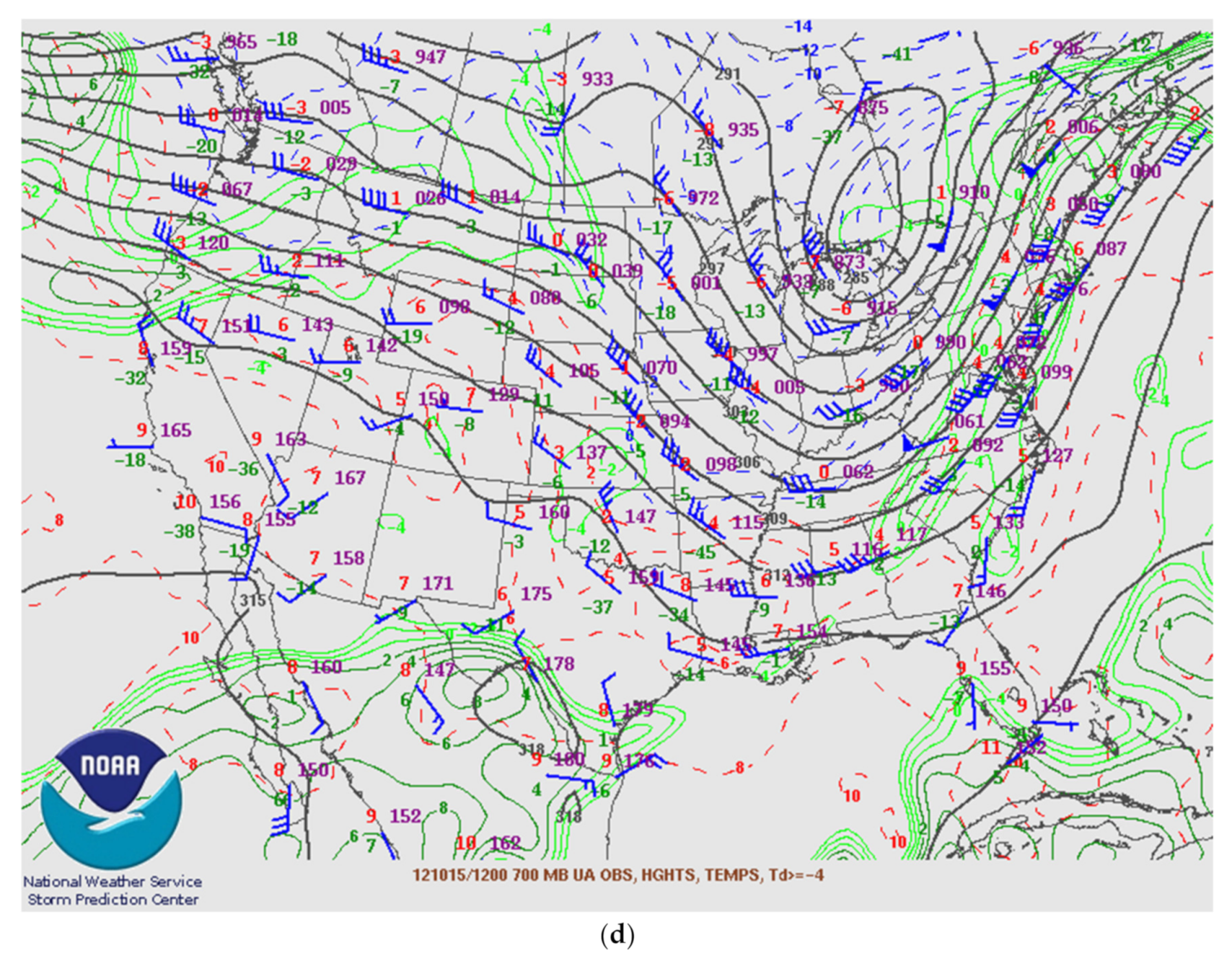
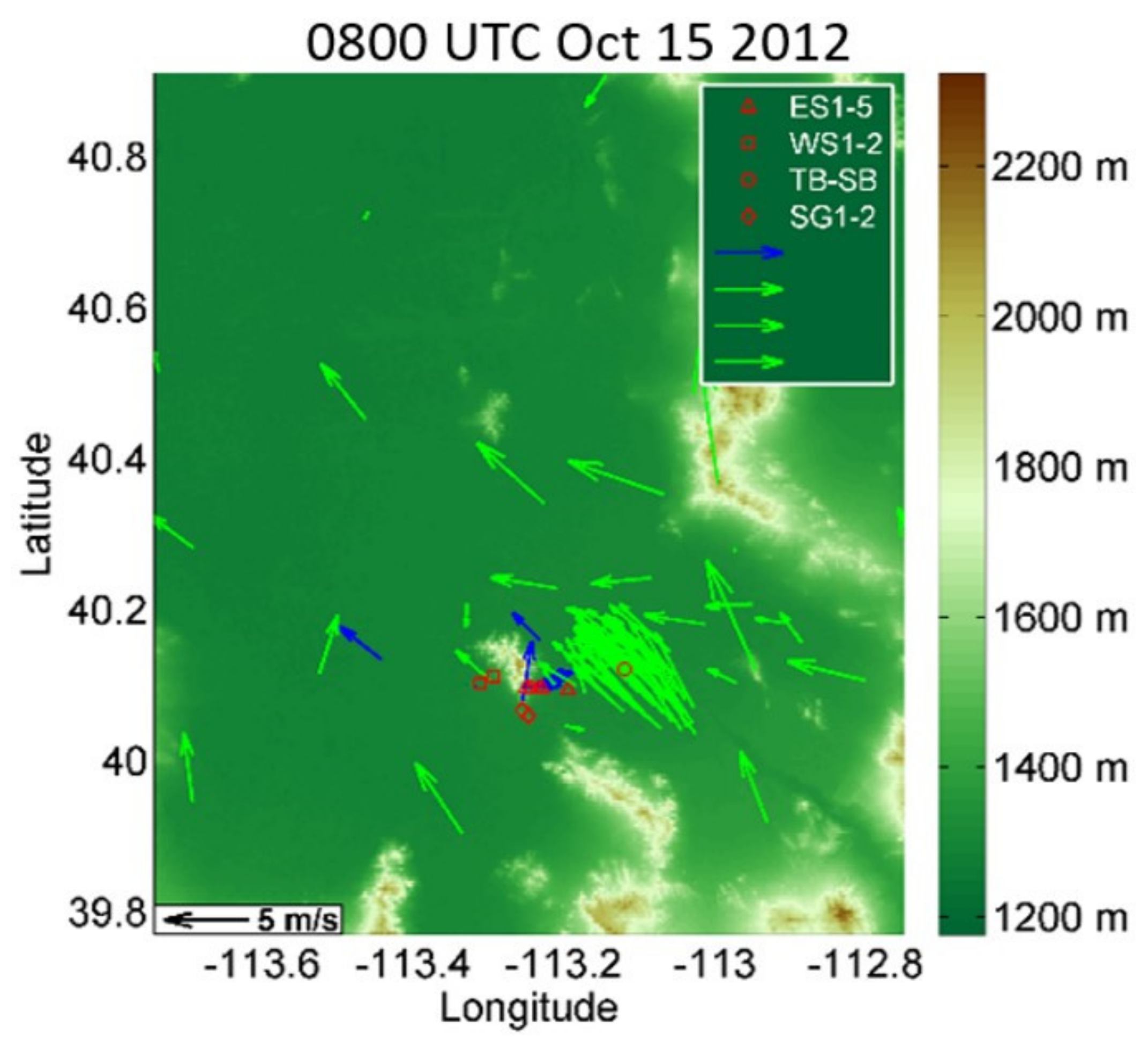
3.1. IOP6 Meteorological Conditions
3.2. Model Experiments
3.2.1. Temperature Comparisons
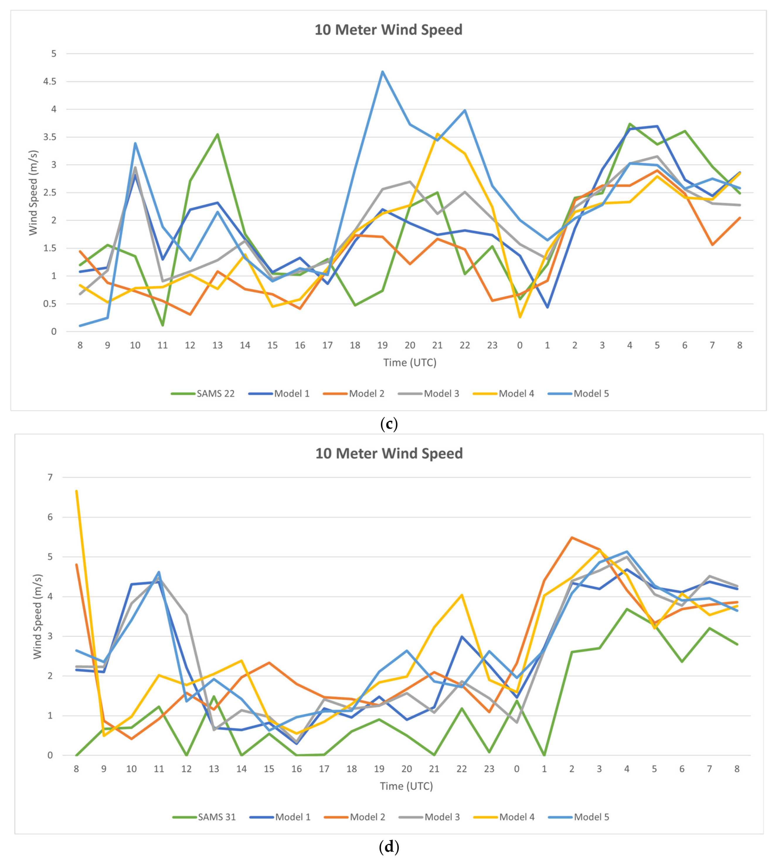
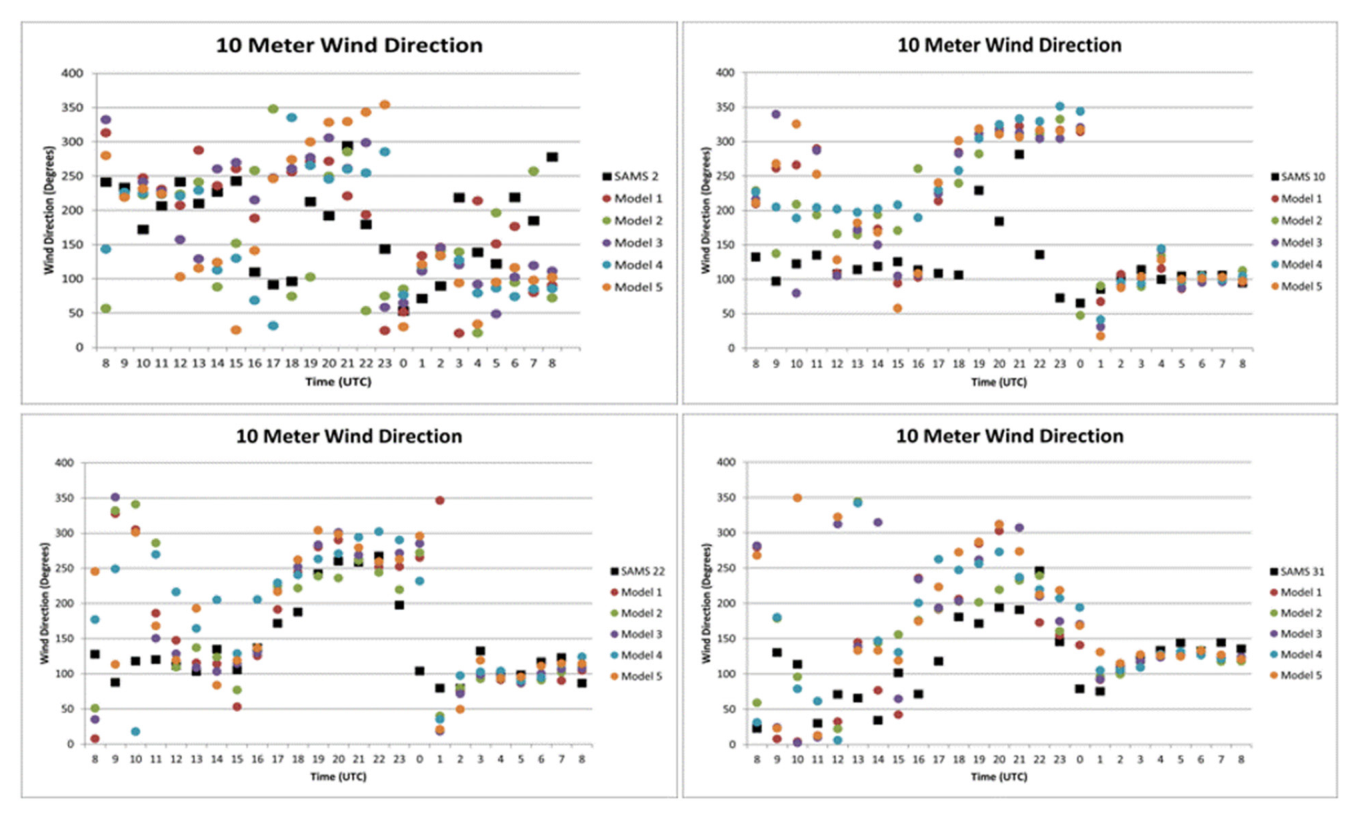
3.2.2. Wind Speed and Wind Direction Comparisons
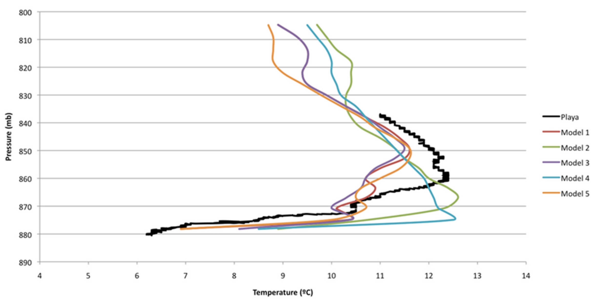
3.2.3. Tethersonde Comparisons
4. Discussion of Modeled Diurnal Thermodynamically Forced Flows
4.1. Playa Breeze
4.2. Katabatic/Anabatic and Upvalley/Downvalley Flows
5. Conclusions
Author Contributions
Funding
Institutional Review Board Statement
Informed Consent Statement
Data Availability Statement
Acknowledgments
Conflicts of Interest
References
- Skamarock, W.C.; Klemp, J.B. A time-split nonhydrostatic atmospheric model for weather research and forecasting applications. J. Comput. Phys. 2008, 227, 3465–3485. [Google Scholar] [CrossRef]
- Crawford, T.; Stensrud, D.; Mora, F.; Merchant, J.; Wetzel, P. Value of incorporating satellite—Derived land cover data in MM5/PLACE for simulating surface temperatures. J. Hydrometeorol. 2001, 2, 453–468. [Google Scholar] [CrossRef]
- Yu, M.; Carmichael, G.R.; Cheng, Y.F. Sensitivity of predicted pollutant levels to urbanization in China. Atmos. Environ. 2012, 60, 544–554. [Google Scholar]
- Hawkes, H.B. Mountain and Valley Winds with Special Reference to the Diurnal Mountain Winds of the Great Salt Lake Region. Ph.D. Thesis, Ohio State University, Columbus, OH, USA, 1947; p. 312. [Google Scholar]
- Hocut, C.; Liberzon, D.; Fernando, H. Separation of upslope flow over a uniform slope. J. Fluid Mech. 2015, 775, 266–287. [Google Scholar] [CrossRef]
- Poulos, G.S. The Interaction of Katabatic Winds and Mountain Waves. Ph.D. Thesis, Colorado State University, Fort Collins, CO, USA, 1996; p. 297. [Google Scholar]
- Fedorovich, E.; Shapiro, A. Structure of numerically simulated katabatic and anabatic flows along steep slopes. Acta Geophys. 2009, 57, 981–1010. [Google Scholar] [CrossRef]
- Drake, S.; Higgins, C.; Pardyjak, E. Distinguishing Time Scales of Katabatic Flow in Complex Terrain. Atmosphere 2021, 12, 1651. [Google Scholar] [CrossRef]
- Defant, F. Local Winds. In Compendium of Meteorology; Malone, T.F., Ed.; American Meteorological Society: Boston, MA, USA, 1951. [Google Scholar]
- Barr, S.; Orgill, M. Influence of External Meteorology on Nocturnal Valley Drainage Winds. J. Appl. Meteorol. 1989, 28, 497–517. [Google Scholar] [CrossRef]
- Mahrt, L.; Larsen, S. Relation of slope winds to the ambient flow over gentle terrain. Bound. Layer Meteorol. 1990, 53, 93–102. [Google Scholar] [CrossRef]
- Mursch-Radlgruber, E. Observations of flow structure in a small forested valley system. Theor. Appl. Climatol. 1995, 52, 3–17. [Google Scholar] [CrossRef]
- Poulos, G.; Bossert, J.T.; Pielke, R.S. The Interaction of Katabatic Flow and Mountain Waves. Part I: Observations and Idealized Simulations. J. Atmos. Sci. 2000, 57, 1919–1936. [Google Scholar] [CrossRef]
- Serafin, S.; De Wekker, S.; Knievel, J. A Mesoscale Model—Based Climatography of Nocturnal Boundary—Layer Characteristics over the Complex Terrain of North—Western Utah. Bound. Layer Meteorol. 2015, 159, 495–519. [Google Scholar] [CrossRef]
- Rife, D.L.; Warner, T.; Chen, F.; Astling, E.G. Mechanisms for Diurnal Boundary Layer Circulations in the Great Basin Desert. Mon. Weather Rev. 2002, 130, 921–938. [Google Scholar] [CrossRef]
- Whiteman, C.D. Mountain Meteorology: Fundamentals and Applications; Oxford University Press: Oxford, UK, 2000; p. 355. [Google Scholar]
- Thyer, N. A theoretical explanation of mountain and valley winds by a numerical method. Arch. Für Meteorol. Geophys. Und Bioklimatol. Ser. A 1966, 15, 318–348. [Google Scholar] [CrossRef]
- Demko, J.C.; Geerts, B. A Numerical Study of the Evolving Convective Boundary Layer and Orographic Circulation around the Santa Catalina Mountains in Arizona Part I: Circulation without Deep Convection. Mon. Weather Rev. 2010, 138, 1902–1922. [Google Scholar]
- Gleeson, T.A. Effects of Various Factors on Valley Winds. J. Atmos. Sci. 1953, 10, 262–269. [Google Scholar] [CrossRef]
- Rampanelli, G.; Zardi, D.; Rotunno, R. Mechanisms of Up-Valley Winds. J. Atmos. Sci. 2004, 61, 3097–3111. [Google Scholar] [CrossRef]
- Chiao, S.; Dumais, R. A down-valley low-level jet event during T-REX 2006. Meteorol. Atmos. Phys. 2013, 122, 75–90. [Google Scholar] [CrossRef]
- De Wekker, S.; Liu, Y.; Knievel, J.; Pal, S.; Emmitt, G.D. Observations and Simulations of the Wind Structure in the Boundary Layer around an Isolated Mountain during the Materhorn Field Experiment. In Proceedings of the American Geophysical Union Meeting, San Francisco, CA, USA, 9–13 December 2013. [Google Scholar]
- Bluestein, H. Synoptic—Dynamic Meteorology in Midlatitudes Volume 1 Principles of Kinematics and Dynamics; Oxford University Press: New York, NY, USA, 1992. [Google Scholar]
- Tapper, N.J. Evidence for a mesoscale thermal circulation over dry salt lakes. Palaeogeogr. Paleoclimatol. Paleoecol. 1991, 84, 259–269. [Google Scholar] [CrossRef]
- Physick, W.L.; Tapper, N.J. A Numerical Study of Circulations Induced by a Dry Salt Lake. Mon. Weather Rev. 1990, 118, 1029–1042. [Google Scholar] [CrossRef]
- Pleim, J.; Ran, L.; Gilliam, R. New High-Resolution Land—Use Data in WRF. In Proceedings of the 10th WRF User’s Workshop, Boulder, CO, USA, 23–26 June 2009. [Google Scholar]
- Massey, J.; Steenburgh, J.; Hoch, S.; Knievel, J. Sensitivity of near—surface temperature forecasts to soil properties over a sparsely vegetated dryland region. J. Appl. Meteorol. Climatol. 2014, 53, 1976–1995. [Google Scholar] [CrossRef]
- Dimitrova, R.; Silver, Z.; Fernando, H.; Leo, L.; DiSabatino, S.; Hocut, C.; Zsedrovits, T. Intercomparison between Different PBL Options in WRF Model: Modification of 2 PBL Schemes for Stable Conditions. In Proceedings of the 94th Annual Meeting of the American Meteorological Society (AMS), Atlanta, GA, USA, 2–6 February 2014; p. 7. [Google Scholar]
- Pal, S.; De Wekker, S.; Emmitt, G. Investigation of the Spatial Variability of the Convective Boundary Layer Heights over an Isolated Mountain: Cases from the MATERHORN-2012 Experiment. J. Appl. Meteorol. Climatol. 2016, 55, 1927–1952. [Google Scholar] [CrossRef]
- Shin, H.H.; Dudhia, J. Evaluation of PBL Parameterizations in WRF at Subkilometer Grid Spacings: Turbulence Statistics in the Dry Convective Boundary Layer. Mon. Weather Rev. 2016, 144, 1161–1177. [Google Scholar] [CrossRef]
- Njuki, S.M.; Mannaerts, C.M.; Su, Z. Influence of Planetary Boundary Layer (PBL) Parameterizations in the Weather Research and Forecasting (WRF) Model on the Retrieval of Surface Meteorological Variables over the Kenyan Highlands. Atmosphere 2022, 13, 169. [Google Scholar] [CrossRef]
- Cheng-Gang, W.; Ying-Jie, S.; Feng, L.; Le, C.; Jia-De, Y.; Hai-Mei, J. Comparison and analysis of several planetary boundary layer schemes in WRF model between clear and overcast days. Chin. J. Geophys. 2017, 60, 141–153. [Google Scholar] [CrossRef]
- Cohen, A.E.; Cavallo, S.M.; Coniglio, M.C.; Brooks, H.E. A review of planetary boundary layer parameterization schemes and their sensitivity in simulating southeastern U.S. cold season severe weather environments. Weather Forecast. 2015, 30, 591–612. [Google Scholar]
- Hong, S.-Y.; Yign, N.; Jimy, D. A new vertical diffusion package with an explicit treatment of entrainment processes. Mon. Weather Rev. 2006, 134, 2318–2341. [Google Scholar] [CrossRef] [Green Version]
- Wyszogrodzki, A.A.; Liu, Y.; Jacobs, N.; Childs, P.; Zhang, Y.; Roux, G.; Warner, T.T. Analysis of the surface temperature and wind forecast errors of the NCAR-AirDat operational CONUS 4-km WRF forecasting system. Meteorol. Atmos. Phys. 2013, 122, 125–143. [Google Scholar] [CrossRef] [Green Version]
- Xu, H.; Wang, Y.; Wang, M. The Performance of a Scale-Aware Nonlocal PBL Scheme for the Subkilometer Simulation of a Deep CBL over the Taklimakan Desert. Adv. Meteorol. 2018, 2018, 8759594. [Google Scholar] [CrossRef] [Green Version]
- Skamarock, W.C.; Snyder, C.; Klemp, J.B.; Park, S. Vertical Resolution Requirements in Atmospheric Simulation. Mon. Weather Rev. 2019, 147, 2641–2656. [Google Scholar] [CrossRef]
- Fernando, H.J.S. Coauthors. The MATERHORN–Unraveling the Intricacies of Mountain Weather. Bull. Am. Meteorol. Soc. 2015, 96, 1945–1967. [Google Scholar] [CrossRef]
- Fernando, H.J.S.; Pardyjak, E.R. Field Studies Delve into the Intricacies of Mountain Weather. EOS 2013, 94, 313–315. [Google Scholar] [CrossRef]
- Janjic, Z. Nonsingular Implementation of the Mellor—Yamada Level 2.5 Scheme in the NCEP Meso Model; NCEP Office Note; National Centers for Environmental Prediction: College Park, MD, USA, 2001; p. 437.
- Grachiev, A.A.; Fairall, C.W. Dependence of the Monin—Obukhov Stability Parameter on the Bulk Richardson Number over the Ocean. J. Appl. Meteorol. 1996, 36, 406–414. [Google Scholar] [CrossRef]
- Chen, F.; Dudhia, J. Coupling an Advanced Surface—Hydrology Model with the Penn State—NCAR MM5 Modeling System. Part I: Model Implementation and Sensitivity. Mon. Weather Rev. 2001, 129, 569–585. [Google Scholar] [CrossRef]
- Ek, M.B.; Mitchell, K.; Lin, Y.; Rogers, E.; Grunmann, P.; Koren, V.; Gayno, G.; Tarpley, J.D. Implementation of Noah land surface model advances in the National Centers for Environmental Prediction operational mesoscale Eta model. J. Geophys. Res. 2003, 108, 8851. [Google Scholar] [CrossRef]
- Tewari, M.; Chen, F.; Wang, W.; Dudhia, J.; LeMone, M.; Mitchell, K.; Ek, M.; Gayno, G.; Wegiel, J.; Cuenca, R.H. Implementation and Verification of the Unified NOAH Land Surface Model in the WRF Model. In Proceedings of the 20th Conference on Weather Analysis and Forecasting/16th Conference on Numerical Weather Prediction, Seattle, WA, USA, 10–16 January 2004; pp. 11–15. [Google Scholar]
- Shin, H.H.; Hong, S.; Dudhia, J.; Kim, Y. Orography—Induced Gravity Wave Drag Parameterization in the Global WRF: Implementation and Sensitivity to Shortwave Radiation Schemes. Adv. Meteorol. 2010, 2010, 959014. [Google Scholar] [CrossRef] [Green Version]
- Zangl, G. An Improved Method for Computing Horizontal Diffusion in a Sigma–Coordinate Model and Its Application to Simulations over Mountainous Topography. Mon. Weather Rev. 2002, 130, 1423–1432. [Google Scholar] [CrossRef]
- Mlawer, E.J.; Taubman, S.; Brown, P.; Iacono, M.; Clough, S.A. Radiative transfer for inhomogeneous atmospheres: RRTM, a validated correlated—k model for the longwave. J. Geophys. Res. 1997, 102, 663–682. [Google Scholar] [CrossRef] [Green Version]
- Thompson, G.; Field, P.; Rasmussen, R.; Hall, W. Explicit Forecasts of Winter Precipitation Using an Improved Bulk Microphysics Scheme. Part II: Implementation of a New Snow Parameterization. Mon. Weather Rev. 2008, 136, 5095–5115. [Google Scholar] [CrossRef]
- Kain, J.S. The Kain–Fritsch convective parameterization: An update. J. Appl. Meteorol. 2004, 43, 170–181. [Google Scholar] [CrossRef]
- Arthur, R.S.; Lundquist, K.A.; Olson, J.B. Improved Prediction of Cold-Air Pools in the Weather Research and Forecasting Model Using a Truly Horizontal Diffusion Scheme for Potential Temperature. Mon. Weather Rev. 2021, 149, 155–171. [Google Scholar] [CrossRef]
- Knievel, J.C.; Bryan, G.; Hacker, J.P. Explicit Numerical Diffusion in the WRF Model. Mon. Weather Rev. 2007, 135, 3808–3824. [Google Scholar] [CrossRef]
- Dudhia, J. Reply. Mon. Weather Rev. 1995, 123, 2573–2575. [Google Scholar] [CrossRef]
- Janjic, Z.; Gall, R. Nonhydrostatic Multiscale Model on the B grid (NMMB). Part 1 Dynamics; NCAR Technical Note; University Corporation for Atmospheric Research: Boulder, CO, USA, 2012. [Google Scholar]
- Loveland, T.R.; Merchant, J.W.; Reed, B.C.; Brown, J.F.; Ohlen, D.O.; Olson, P.; Hutchinson, J. Seasonal land cover regions of the United States. Ann. Assoc. Am. Geogr. 1995, 85, 339–355. [Google Scholar] [CrossRef]
- Miller, D.; White, R. A Conterminous United States Multilayer Soil Characteristics Dataset for Regional Climate and Hydrology Modeling. Earth Interact. 1998, 2, 1–26. [Google Scholar] [CrossRef]
- Fry, J.; Xian, G.; Jin, S.; Dewitz, J.; Homer, C.; Yang, L.; Barnes, C.; Herold, N.; Wickham, J. Completion of the 2006 National Land Cover Database for the Conterminous United States. Photogramm. Eng. Remote Sens. 2011, 77, 858–864. [Google Scholar]
- Hennig, T.A.; Kretsch, J.; Pessagno, C.; Salamonowicz, P.; Stein, W. The Shuttle Radar Topography Mission. Digit. Earth Moving. Lect. Notes Comput. Sci. 2001, 2181, 65–77. [Google Scholar]
- Environmental Modeling Center. The GFS Atmospheric Model. NCEP Office Note 442, Global Climate and Weather Modeling Branch; EMC: Camp Springs, MD, USA, 2003. [Google Scholar]
- Galperin, B.; Sukoriansky, S. Progress in turbulence parameterization for geophysical flows. In Proceedings of the 3rd International Workshop on Next-Generation NWP Models: Bridging Parameterization, Explicit Clouds, and Large Eddies, Seoul, Republic of Korea, 4 May 2010. [Google Scholar]
- Chou, M.D.; Suarez, M.J. A solar radiation parameterization for atmospheric studies. NASA Tech. Memo. 1999, 40, 104606. [Google Scholar]
- Chou, M.D.; Suarez, M.; Liang, X.; Yan, M.M.H. A thermal infrared radiation parameterization for atmospheric studies. NASA Tech. Memo. 2001, 68, 104606. [Google Scholar]
- McCumber, M.; Pielke, R.A., Sr. Simulation of the Effects of Surface Fluxes of Heat and Moisture in a Mesoscale Numerical Model 1. Soil Layer. J. Geophys. Res. 1981, 86, 9929–9938. [Google Scholar] [CrossRef] [Green Version]
- Johansen, O. Thermal Conductivity of Soils. Ph.D. Thesis, Norwegian University of Science and Technology, Trondheim, Norway, 1975; p. 291. [Google Scholar]
- Lehner, M.; Whiteman, C.; Hoch, S.; Jensen, D.; Pardyjak, E.; Leo, L.; Di Sabatino, S.; Fernando, H.J.S. A Case Study of the Nocturnal Boundary Layer Evolution on a Slope at the Foot of a Desert Mountain. J. Appl. Meteorol. Climatol. 2015, 54, 732–751. [Google Scholar] [CrossRef]
- Jeglum, M.E.; Hoch, S. Multiscale Characteristics of Surface Winds in an Area of Complex Terrain in Northwest Utah. J. Appl. Meteorol. Climatol. 2016, 55, 1549–1563. [Google Scholar] [CrossRef]
- Rodrigues, C.V.; Palma, J.M.L.M. Estimation of turbulence intensity and shear factor for diurnal and nocturnal periods with an URANS flow solver coupled with WRF. J. Phys. Conf. Ser. 2014, 524, 10. [Google Scholar] [CrossRef] [Green Version]
- Massey, J.D.; Steenburgh, W.; Knievel, J.; Cheng, W. Regional Soil Moisture Biases and their Influence on WRF Model Temperature Forecasts over the Intermountain West. Weather Forecast. 2016, 31, 197–216. [Google Scholar] [CrossRef]
- Han, L.; Ding, J.; Zhang, J.; Chen, P.; Wang, J.; Wang, Y.; Wang, J.; Ge, X.; Zhang, Z. Precipitation events determine the spatiotemporal distribution of playa surface salinity in arid regions: Evidence from satellite data fused via the enhanced spatial and temporal adaptive reflectance fusion model. CATENA 2021, 206, 105546. [Google Scholar] [CrossRef]
- Hang, C.; Nadeau, D.; Jensen, D.; Hoch, S.; Pardyjak, E. Playa Soil Moisture and Evaporation Dynamics During the MATERHORN Field Program. Bound. Layer Meteorol. 2016, 159, 521–538. [Google Scholar] [CrossRef]
- Jensen, D.D.; Nadeau, D.; Hoch, S.; Pardyjak, E.R. Observations of near-surface heat-flux and temperature profiles through the early evening transition over contrasting surfaces. Bound. Layer Meteorol. 2016, 159, 567–587. [Google Scholar] [CrossRef]
- Stauffer, D.R. Uncertainty in Environmental NWP Modeling. Handbook of Environmental Fluid Dynamics; Harindra, J., Fernando, S., Eds.; Taylor &Francis Books, Inc.: London, UK, 2011. [Google Scholar]
- Morrison, T.; Calaf, M.; Higgins, C.; Drake, S.; Perelet, A.; Pardyjak, E. The Impact of Surface Temperature Heterogeneity on Near-Surface Heat Transport. Bound. Layer Meteorol. 2021, 180, 247–272. [Google Scholar] [CrossRef]
- Silver, Z.; Dimitrova, R.; Zsedrovits, T.; Baines, P.; Fernando, H. Simulation of Stably Stratified flow in complex terrain: Flow structures and dividing streamline. Environ. Fluid Mech. 2018, 20, 1281–1311. [Google Scholar] [CrossRef]
- Massey, J.D.; Steenburgh, W.; Hoch, S.; Jensen, D. Simulated and Observed Surface Energy Fluxes and Resulting Playa Breezes during the MATERHORN. J. Appl. Meteorol. Climatol. 2017, 56, 915–935. [Google Scholar] [CrossRef]
- Hang, C.; Nadeau, D.; Pardyjak, E.; Parlange, M. A comparison of near-surface potential temperature variance budgets for unstable atmospheric flows with contrasting vegetation cover flat surfaces and a gentle slope. Environ. Fluid Mech. 2020, 20, 1251–1279. [Google Scholar] [CrossRef]
- Duine, G.L.; De Wekker, S. The effects of horizontal grid spacing on simulated daytime boundary layer depths in an area of complex terrain in Utah. Environ. Fluid Mech. 2017, 20, 1313–1331. [Google Scholar] [CrossRef]
- Tijm, A.B.C.; Holtslag, A.A.M.; van Delden, A.J. Observations and Modeling of the Sea-Breeze with the Return Current. Mon. Weather Rev. 1999, 127, 625–640. [Google Scholar] [CrossRef]
- Dimitrova, R.; Silver, Z.; Zsedrovits, T.; Hocut, C.; Leo, L.; Di Sabatino, S.; Fernando, H. Assessment of planetary boundary-layer schemes in the Weather Research and Forecasting mesoscale model using MATERHORN field data. Bound. Layer Meteorol. 2016, 159, 589–609. [Google Scholar] [CrossRef]
- Wyngaard, J.C. Toward Numerical Modeling in the “Terra Incognita”. J. Atmos. Sci. 2004, 61, 1816–1826. [Google Scholar] [CrossRef]
- Ching, J.; Rotunno, R.; LeMone, M.; Martilli, A.; Kosović, B.; Jiménez, P.; Dudhia, J. Convectively induced secondary circulations in fine-grid mesoscale numerical weather prediction models. Mon. Weather Rev. 2014, 42, 3284–3302. [Google Scholar] [CrossRef] [Green Version]
- Rai, R.K.; Berg, L.; Kosović, B.; Haupt, S.; Mirocha, J.; Ennis, B.; Draxl, C. Evaluation of the impact of horizontal grid spacing in terra incognita on coupled mesoscale–microscale simulations using the WRF framework. Mon. Weather Rev. 2019, 147, 1007–1027. [Google Scholar] [CrossRef]
- Haupt, S.E.; Kosović, B.; Shaw, W.; Berg, L.; Churchfield, M.; Cline, J.; Draxl, C.; Ennis, B.; Koo, E.; Kotamarthi, R.; et al. On bridging a modeling scale gap: Mesoscale to microscale coupling for wind energy. Bull. Am. Meteorol. Soc. 2019, 100, 2533–2550. [Google Scholar] [CrossRef]
- Hawbecker, P.; Kosović, B.; Muñoz-Esparza, D.; Sauer, J.; Dudhia, J.; Patton, G. Simulations Across Scales over Complex Terrain: Lessons Learned from a Perdigao Case Study. Joint WRF/MPAS Users’ Workshop 2021 (Virtual), NCAR, June 2021. Available online: https://www2.mmm.ucar.edu/wrf/users/workshops/WS2021/presentation_pdfs/hawbecker.pdf (accessed on 2 December 2022).
- Dai, Y.; Basu, S.; Maronga, B.; de Roode, S.R. Addressing the Grid-Size Sensitivity Issue in Large-Eddy Simulations of Stable Boundary Layers. Bound. Layer Meteorol. 2021, 178, 63–89. [Google Scholar] [CrossRef]
- Seaman, N.L.; Gaudet, B.J.; Stauffer, D.R.; Mahrt, L.; Richardson, S.J.; Zielonka, J.R.; Wyngaard, J.C. Prediction of Submesoscale in the Nocturnal Stable Boundary Layer over Complex Terrain. Mon. Weather Rev. 2012, 140, 956–977. [Google Scholar] [CrossRef] [Green Version]
- Paperman, J.; Potchter, O.; Alpert, P. Characteristics of the summer 3-D katabatic flow in a semi-arid zone—The case of the Dead Sea. Int. J. Climatol. 2022, 42, 1975–1984. [Google Scholar] [CrossRef]
- Serafin, S.; Adler, B.; Cuxart, J.; De Wekker, S.; Gohm, A.; Grisogono, B.; Kalthoff, N.; Kirshbaum, D.; Rotach, M.; Schmidli, J.; et al. Exchange Processes in the Atmospheric Boundary Layer Over Mountainous Terrain. Atmosphere 2018, 9, 32. [Google Scholar] [CrossRef] [Green Version]
- Lee, T.R.; Buban, M. Evaluation of Monin–Obukhov and Bulk Richardson Parameterizations for Surface–Atmosphere Exchange. J. Appl. Meteorol. Climatol. 2020, 59, 1091–1107. [Google Scholar] [CrossRef] [Green Version]
- Pilotto, I.L.; Rodríguez, D.A.; Chan Chou, S.; Tomasella, J.; Sampaio, G.; Gomes, J.L. Effects of the surface heterogeneities on the local climate of a fragmented landscape in Amazonia using a tile approach in the Eta/Noah-MP model. Q. J. R. Meteorol. Soc. 2017, 143, 1565–1580. [Google Scholar] [CrossRef]
- Arsenault, K.R.; Nearing, G.S.; Wang, S.; Yatheendradas, S.; Peters-Lidard, C.D. Parameter Sensitivity of the Noah-MP Land Surface Model with Dynamic Vegetation. J. Hydrometeorol. 2018, 19, 815–830. [Google Scholar] [CrossRef]
- Beck, J.; Brown, J.; Dudhia, J.; Gill, D.; Hertneky, T.; Klemp, J.; Wang, W.; Williams, C.; Hu, M.; James, E.; et al. An Evaluation of a Hybrid, Terrain-Following Vertical Coordinate in the WRF-Based RAP and HRRR Models. Weather Forecast. 2020, 35, 1081–1096. [Google Scholar] [CrossRef] [Green Version]
- Daniels, M.; Lundquist, K.; Mirocha, J.; Wiersema, D.; Chow, F. A New Vertical Grid Nesting Capability in the Weather Research and Forecasting (WRF) Model. Mon. Weather Rev. 2016, 144, 3725–3747. [Google Scholar] [CrossRef]


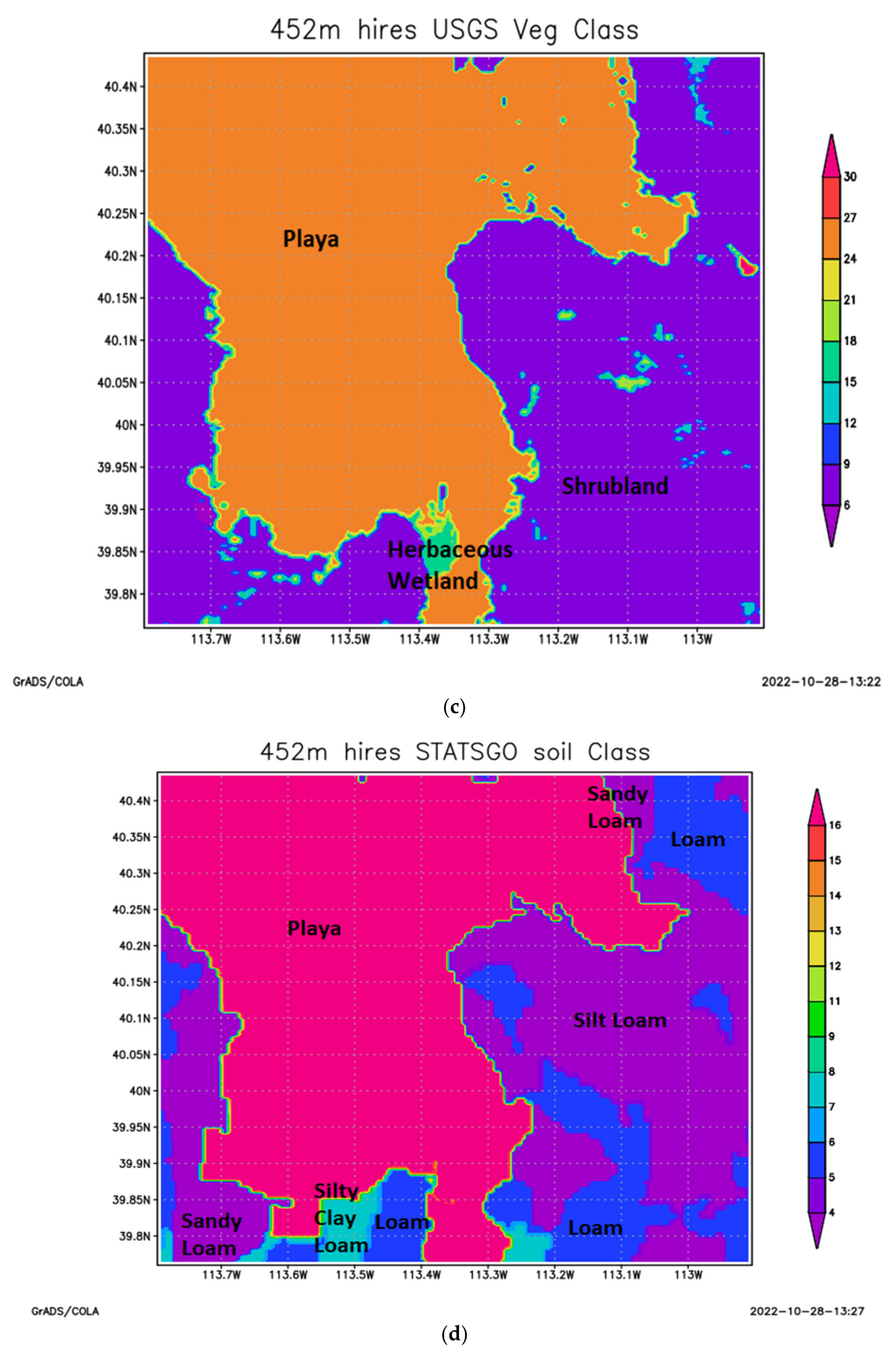
| MS1 | MS2 | MS3 | MS4 | MS5 | |
|---|---|---|---|---|---|
| Land Use and Soil Texture | USGS GTOPO30 (30 arc sec; 24 categories) and STATSGO 30 arc sec with 16 soil categories (no playa) | NLCD 2006 (1 arc sec; 27 categories) and STATSGO 30 arc sec with 19 soil categories (includes playa) | NLCD 2006 (1 arc sec; 27 categories) and STATSGO 30 arc sec with 19 soil categories (includes playa) | NLCD 2006 (1 arc sec; 27 categories) and STATSGO 30 arc sec with 19 soil categories (includes playa) | NLCD 2006 (1 arc sec; 27 categories) and STATSGO 30 arc sec with 19 soil categories (includes playa) |
| Boundary-Layer Physics | MYJ | MYJ | MYJ | QNSE | QNSE |
| Initial/Lateral Boundary Conditions | NAM 12- -km from NCEP | GFS ½ degree from NCEP | NAM 12- -km from NCEP | GFS ½ degree model NCEP | NAM 12- -km from NCEP |
| Turbulent Diffusion | Horizontal diffusion on terrain following surfaces | Horizontal diffusion on terrain following surfaces | Horizontal diffusion on terrain following surfaces | Horizontal diffusion on Cartesian z-following surfaces | Horizontal diffusion on Cartesian z-following surfaces |
| Radiation | Dudhia option for shortwave and RRTM for long wave | Dudhia option for shortwave and RRTM for long wave | Dudhia option for shortwave and RRTM for long wave | Goddard options for short wave and long wave | Goddard options for short wave and long wave |
| Thermal Soil Conductivity Over Sandy and Silt Loam Soil Types | Existing parameterization in Noah land-surface model | Existing parameterization in Noah land-surface model | Existing parameterization in Noah land-surface model | New parameterization in Noah land-surface model | New parameterization in Noah land-surface model |
| SAMS Station | MS1 | MS2 | MS3 | MS4 | MS5 |
|---|---|---|---|---|---|
| OFF PLAYA | |||||
| 2 | 1.96 | 1.90 | 1.75 | 1.09 | 0.71 |
| 10 | 0.96 | 1.55 | 1.02 | 1.09 | −0.05 |
| 22 | 1.45 | 2.12 | 1.67 | 1.31 | 0.12 |
| 31 | −0.36 | 0.15 | −0.26 | 0.15 | −0.18 |
| PLAYA | |||||
| 9 | 0.48 | 0.86 | 0.36 | 0.65 | −0.30 |
| 18 | 0.23 | 0.68 | −0.02 | 0.30 | −0.43 |
| 19 | 0.97 | 1.58 | 0.84 | 1.38 | 0.61 |
| 26 | −0.13 | 0.67 | −0.23 | 0.21 | −0.65 |
| SAMS Station | MS1 | MS2 | MS3 | MS4 | MS5 |
|---|---|---|---|---|---|
| OFF PLAYA | |||||
| 2 | 2.69 | 2.31 | 2.49 | 1.62 | 1.84 |
| 10 | 2.25 | 2.52 | 2.20 | 2.16 | 1.57 |
| 22 | 2.41 | 2.87 | 2.49 | 2.28 | 1.80 |
| 31 | 1.97 | 1.88 | 1.94 | 1.82 | 1.88 |
| PLAYA | |||||
| 9 | 1.31 | 2.02 | 1.69 | 1.81 | 1.47 |
| 18 | 0.93 | 1.59 | 1.34 | 1.37 | 1.41 |
| 19 | 2.11 | 2.83 | 2.36 | 2.81 | 2.55 |
| 26 | 1.09 | 1.97 | 1.52 | 1.80 | 1.42 |
| SAMS Station | MS1 | MS2 | MS3 | MS4 | MS5 |
|---|---|---|---|---|---|
| OFF PLAYA | |||||
| 2 | 0.18 | −0.23 | −0.10 | −0.06 | −0.33 |
| 10 | 1.07 | 1.24 | 1.27 | 1.60 | 1.57 |
| 22 | 0.68 | 0.71 | 0.91 | 1.13 | 1.31 |
| 31 | −0.46 | −0.55 | −0.34 | −0.20 | −0.05 |
| PLAYA | |||||
| 9 | 1.16 | 1.05 | 1.15 | 1.32 | 1.39 |
| 18 | 0.11 | 0.26 | 0.23 | 0.16 | 0.15 |
| 19 | 0.08 | 0.14 | 0.05 | 0.27 | 0.04 |
| 26 | 0.07 | 0.15 | 0.17 | 0.15 | 0.14 |
| SAMS Station | MS1 | MS2 | MS3 | MS4 | MS5 |
|---|---|---|---|---|---|
| OFF PLAYA | |||||
| 2 | 1.10 | 1.44 | 1.26 | 1.81 | 1.46 |
| 10 | 1.32 | 1.34 | 1.42 | 1.63 | 1.66 |
| 22 | 0.93 | 0.99 | 1.05 | 1.18 | 1.41 |
| 31 | 0.99 | 1.02 | 0.94 | 1.26 | 1.08 |
| PLAYA | |||||
| 9 | 1.46 | 1.37 | 1.55 | 1.65 | 1.70 |
| 18 | 1.07 | 1.31 | 1.28 | 1.21 | 1.19 |
| 19 | 1.00 | 1.09 | 0.93 | 1.24 | 1.09 |
| 26 | 0.90 | 1.17 | 0.98 | 1.32 | 1.03 |
| SAMS Station | MS1 | MS2 | MS3 | MS4 | MS5 |
|---|---|---|---|---|---|
| OFF PLAYA | |||||
| 2 | 0.41 | 0.57 | 0.32 | 0.75 | 0.11 |
| 10 | −0.17 | 0.14 | −0.27 | −0.27 | −0.34 |
| 22 | −0.17 | −0.13 | −0.28 | −0.12 | −0.23 |
| 31 | −0.24 | 0.18 | −0.51 | −0.09 | −0.11 |
| PLAYA | |||||
| 9 | 0.17 | 0.15 | 0.01 | −0.09 | 0.11 |
| 18 | −0.87 | −1.18 | −1.07 | −1.18 | −1.33 |
| 19 | −0.95 | −1.55 | −1.03 | −2.01 | −1.45 |
| 26 | −0.48 | −0.69 | −1.10 | −0.66 | −1.00 |
| SAMS Station | MS1 | MS2 | MS3 | MS4 | MS5 |
|---|---|---|---|---|---|
| OFF PLAYA | |||||
| 2 | 1.28 | 1.06 | 1.09 | 1.03 | 0.93 |
| 10 | 0.79 | 0.82 | 0.96 | 1.06 | 1.02 |
| 22 | 0.82 | 0.72 | 0.69 | 0.66 | 0.81 |
| 31 | 1.13 | 1.11 | 1.19 | 1.10 | 1.24 |
| PLAYA | |||||
| 9 | 1.05 | 0.74 | 0.94 | 0.80 | 1.06 |
| 18 | 1.15 | 1.31 | 1.28 | 1.39 | 1.58 |
| 19 | 1.12 | 1.69 | 1.22 | 2.09 | 1.68 |
| 26 | 1.63 | 1.52 | 1.68 | 1.34 | 1.70 |
| SAMS Station | MS1 | MS2 | MS3 | MS4 | MS5 |
|---|---|---|---|---|---|
| OFF PLAYA | |||||
| 2 | 0.90 | 0.92 | 0.93 | 0.97 | 0.93 |
| 10 | 0.97 | 0.98 | 0.98 | 0.99 | 0.97 |
| 22 | 0.97 | 0.98 | 0.98 | 0.98 | 0.95 |
| 31 | 0.95 | 0.93 | 0.95 | 0.93 | 0.92 |
| PLAYA | |||||
| 9 | 0.98 | 0.97 | 0.97 | 0.97 | 0.96 |
| 18 | 0.99 | 0.97 | 0.98 | 0.98 | 0.97 |
| 19 | 0.99 | 0.97 | 0.98 | 0.98 | 0.98 |
| 26 | 0.97 | 0.96 | 0.96 | 0.95 | 0.97 |
| SAMS Station | MS1 | MS2 | MS3 | MS4 | MS5 |
|---|---|---|---|---|---|
| OFF PLAYA | |||||
| 2 | 0.52 | 0.43 | 0.50 | 0.25 | 0.42 |
| 10 | 0.72 | 0.81 | 0.77 | 0.81 | 0.80 |
| 22 | 0.84 | 0.80 | 0.83 | 0.84 | 0.80 |
| 31 | 0.82 | 0.78 | 0.87 | 0.76 | 0.84 |
| PLAYA | |||||
| 9 | 0.68 | 0.61 | 0.66 | 0.44 | 0.65 |
| 18 | 0.61 | 0.51 | 0.43 | 0.56 | 0.64 |
| 19 | 0.28 | 0.19 | 0.18 | 0.20 | 0.22 |
| 26 | 0.80 | 0.72 | 0.80 | 0.79 | 0.80 |
| SAMS Station | MS1 | MS2 | MS3 | MS4 | MS5 |
|---|---|---|---|---|---|
| OFF PLAYA | |||||
| 2 | 0.21 | 0.54 | 0.35 | 0.63 | 0.52 |
| 10 | 0.25 | 0.43 | 0.24 | 0.48 | 0.35 |
| 22 | 0.20 | 0.21 | 0.38 | 0.45 | 0.43 |
| 31 | 0.45 | 0.32 | 0.52 | 0.36 | 0.44 |
| PLAYA | |||||
| 9 | 0.03 | 0.30 | 0.19 | 0.30 | 0.20 |
| 18 | 0.67 | 0.72 | 0.72 | 0.59 | 0.50 |
| 19 | 0.83 | 0.71 | 0.86 | 0.70 | 0.80 |
| 26 | 0.15 | -0.18 | −0.21 | −0.05 | −0.13 |
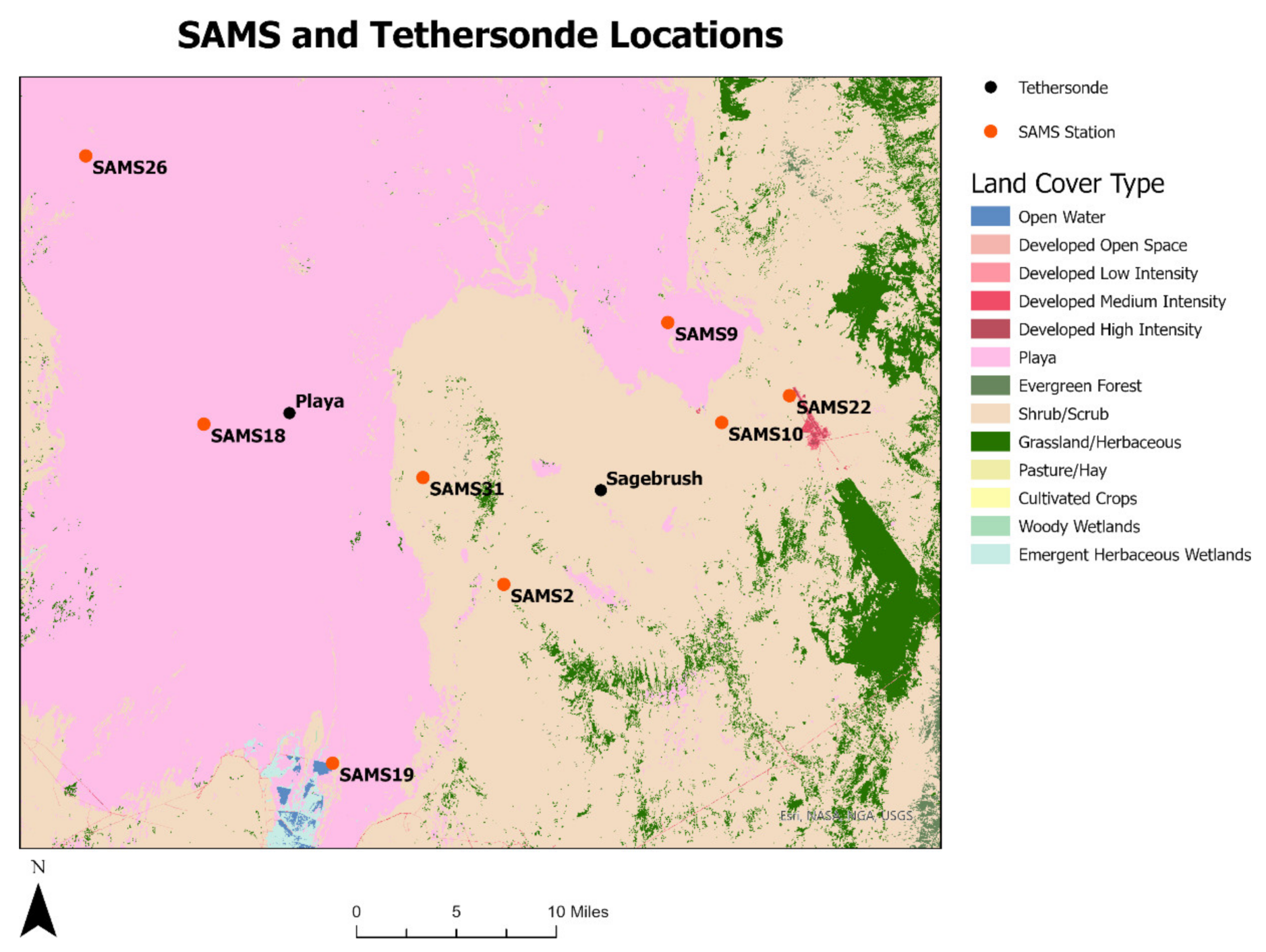
| SAMS Station | Latitude | Longitude | Elevation |
|---|---|---|---|
| OFF PLAYA | Deg N | Deg W | m ASL |
| 2 | 40.046 | −113.208 | 1317.5 |
| 10 | 40.182 | −113.022 | 1314.7 |
| 22 | 40.208 | −112.960 | 1321.0 |
| 31 | 40.108 | −113.307 | 1308.8 |
| PLAYA | |||
| 9 | 40.243 | −113.093 | 1309.8 |
| 18 | 40.116 | −113.533 | 1294.9 |
| 19 | 39.904 | −113.344 | 1306.1 |
| 26 | 40.282 | −113.700 | 1292.0 |
Disclaimer/Publisher’s Note: The statements, opinions and data contained in all publications are solely those of the individual author(s) and contributor(s) and not of MDPI and/or the editor(s). MDPI and/or the editor(s) disclaim responsibility for any injury to people or property resulting from any ideas, methods, instructions or products referred to in the content. |
© 2023 by the authors. Licensee MDPI, Basel, Switzerland. This article is an open access article distributed under the terms and conditions of the Creative Commons Attribution (CC BY) license (https://creativecommons.org/licenses/by/4.0/).
Share and Cite
Dumais, R.E., Jr.; Spade, D.M.; Gill, T.E. Simulations of Mesoscale Flow Systems around Dugway Proving Ground Using the WRF Modeling System. Atmosphere 2023, 14, 251. https://doi.org/10.3390/atmos14020251
Dumais RE Jr., Spade DM, Gill TE. Simulations of Mesoscale Flow Systems around Dugway Proving Ground Using the WRF Modeling System. Atmosphere. 2023; 14(2):251. https://doi.org/10.3390/atmos14020251
Chicago/Turabian StyleDumais, Robert E., Jr., Daniela M. Spade, and Thomas E. Gill. 2023. "Simulations of Mesoscale Flow Systems around Dugway Proving Ground Using the WRF Modeling System" Atmosphere 14, no. 2: 251. https://doi.org/10.3390/atmos14020251