

Medicane Ianos: 4D-Var Data Assimilation of Surface and Satellite Observations into the Numerical Weather Prediction Model WRF

Abstract
:1. Introduction
2. Materials and Methods
2.1. Modeling System
2.2. Assimilation and Verification of Data
2.3. Methodology
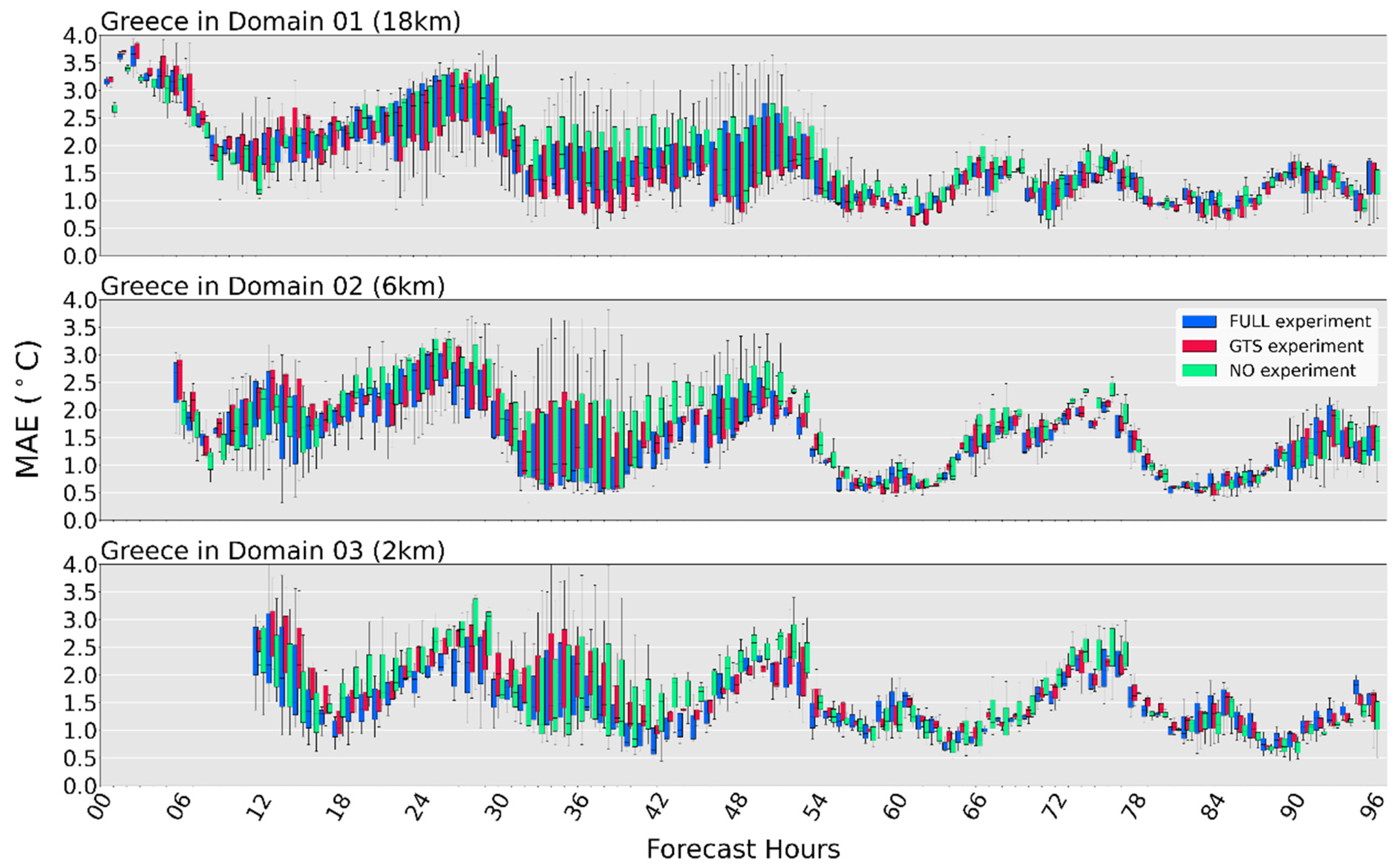
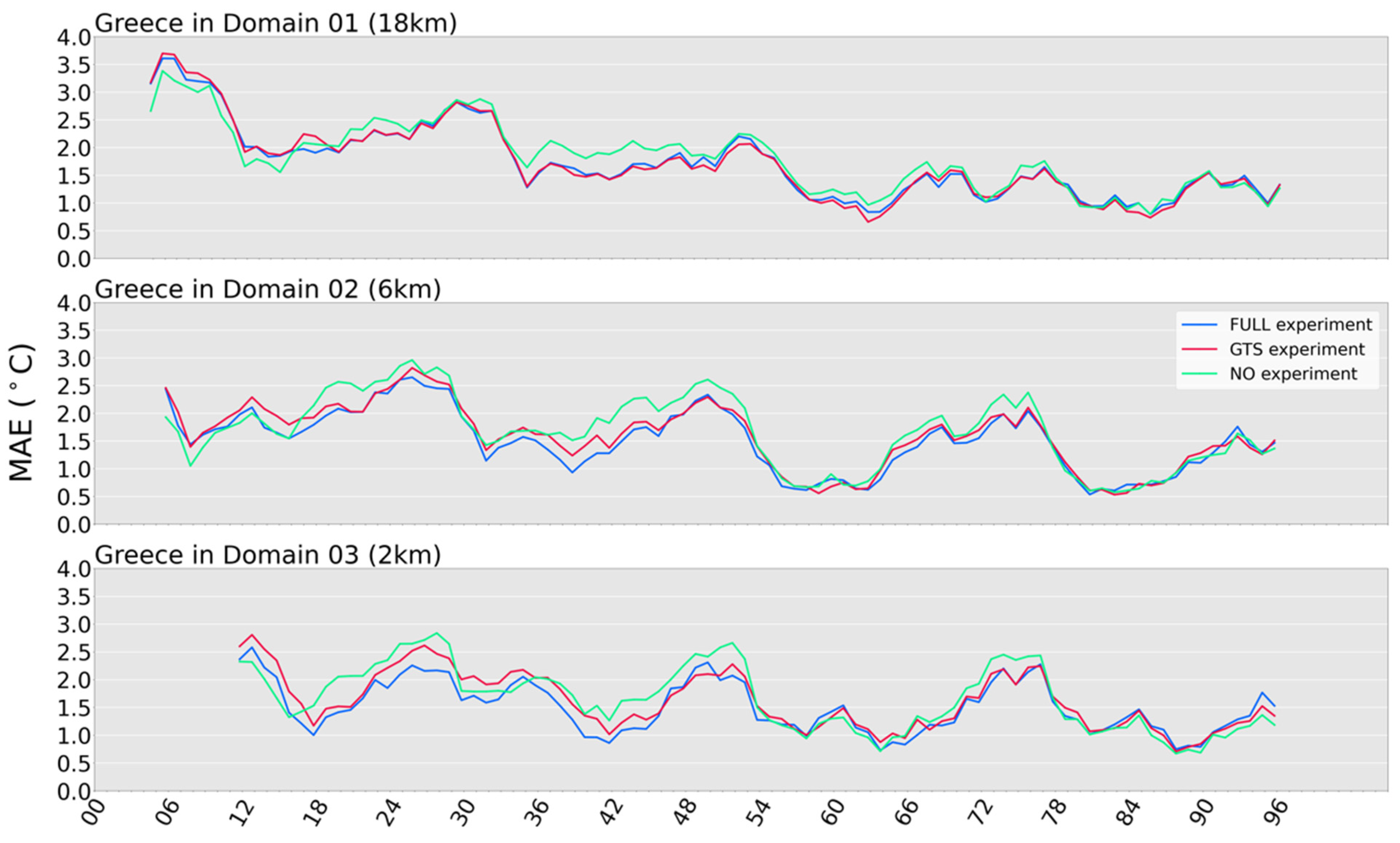
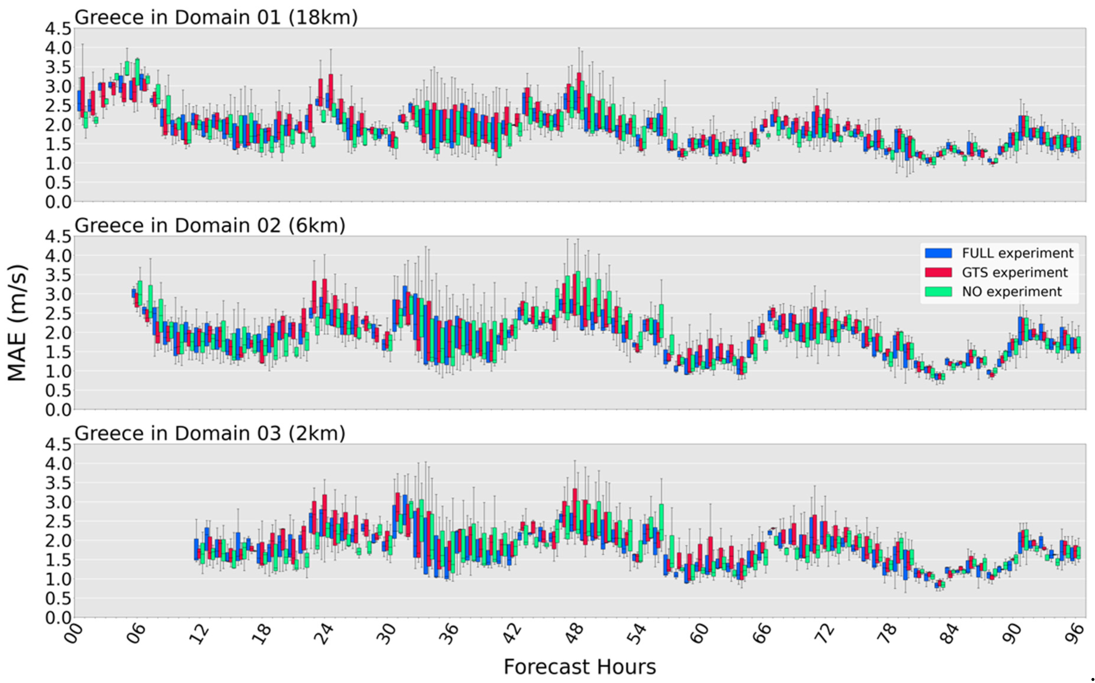
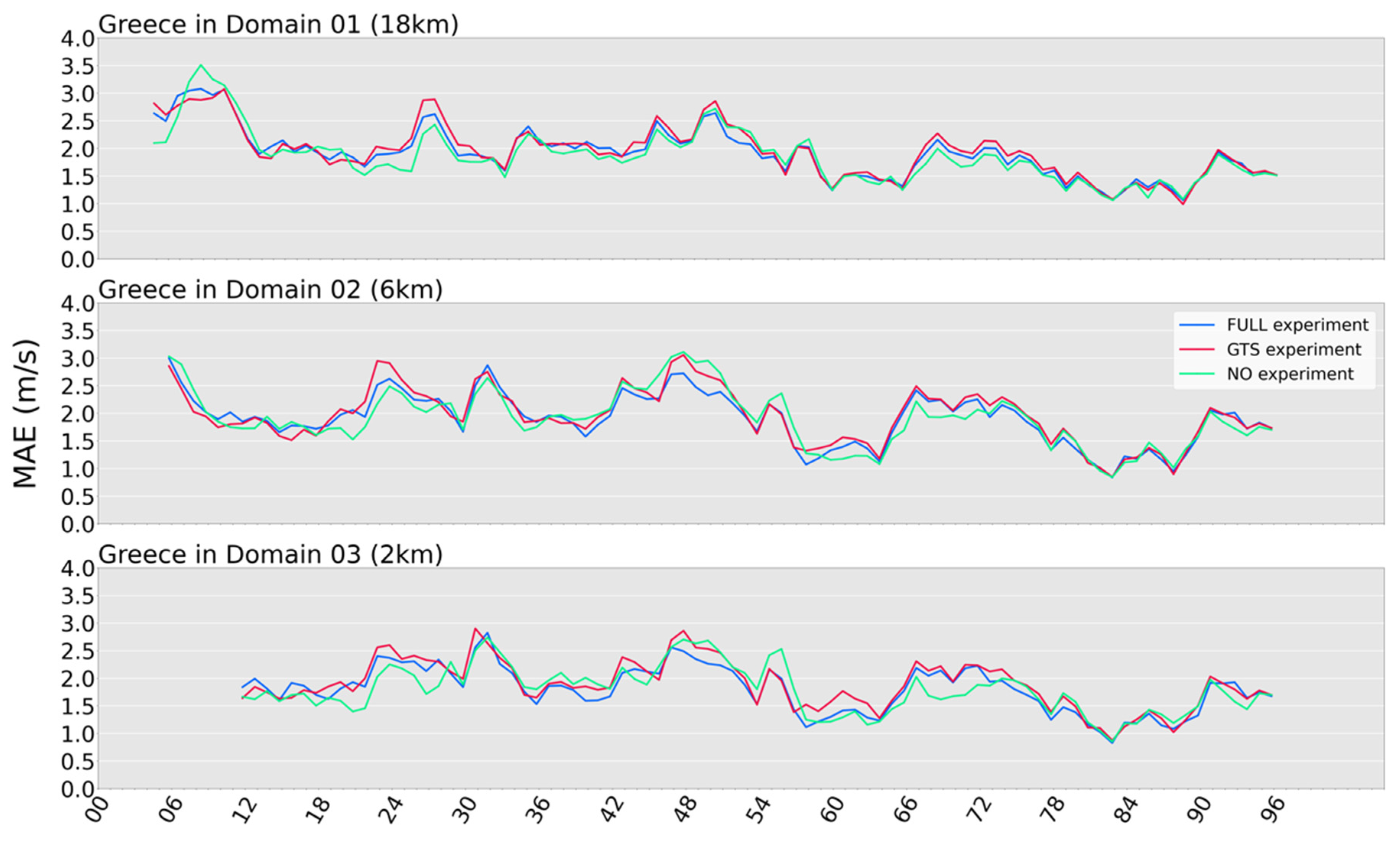
3. Results
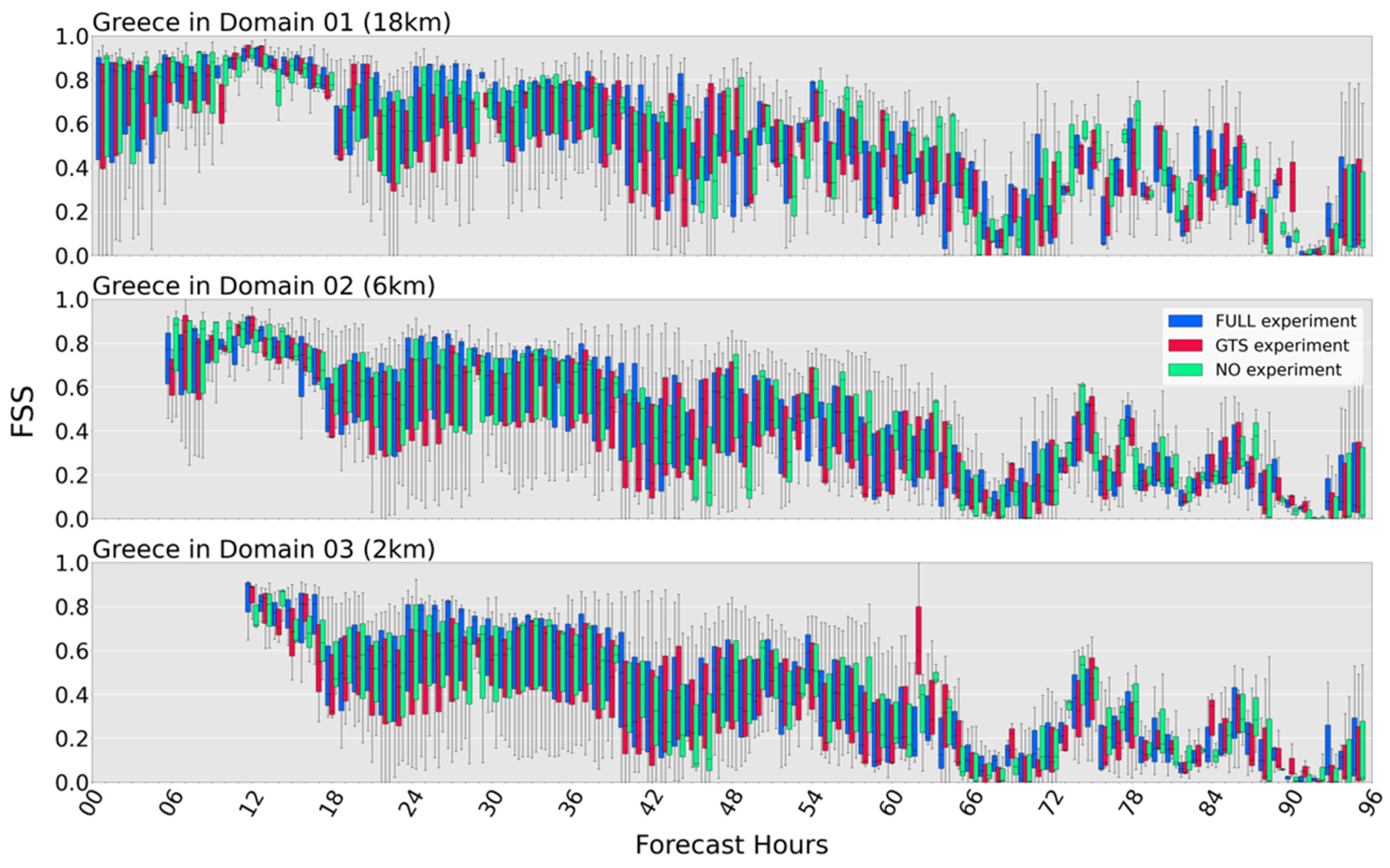
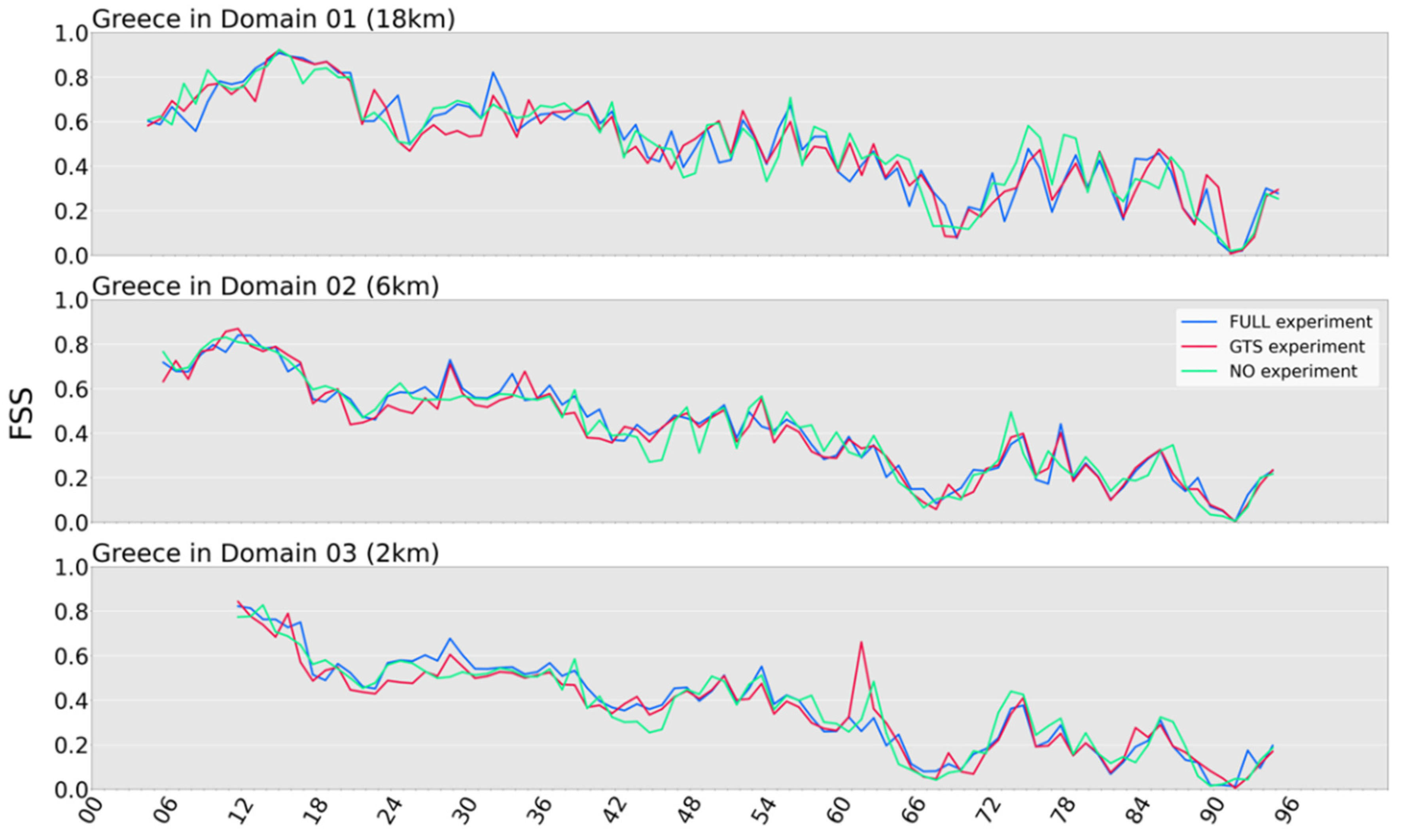
Aggregated Statistics
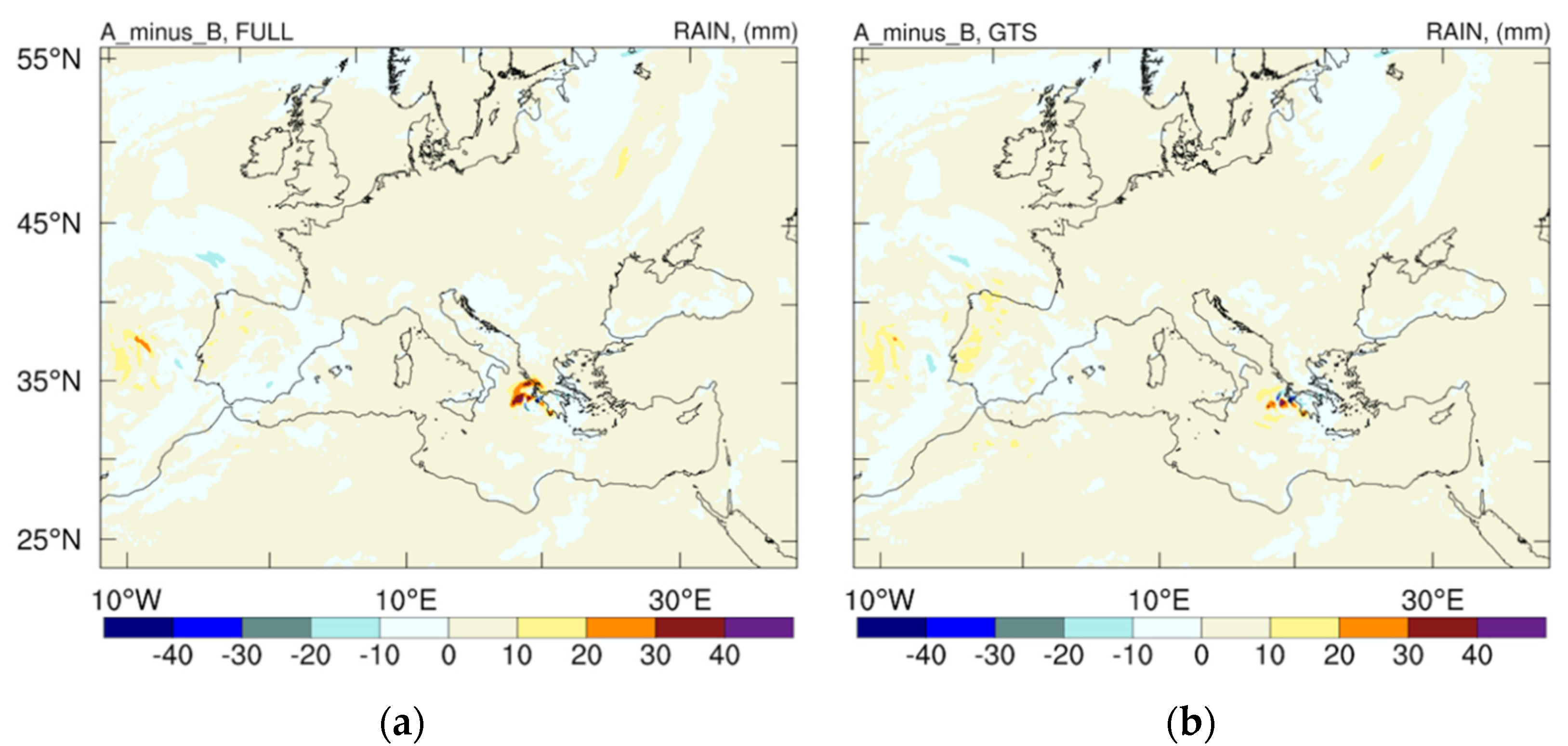
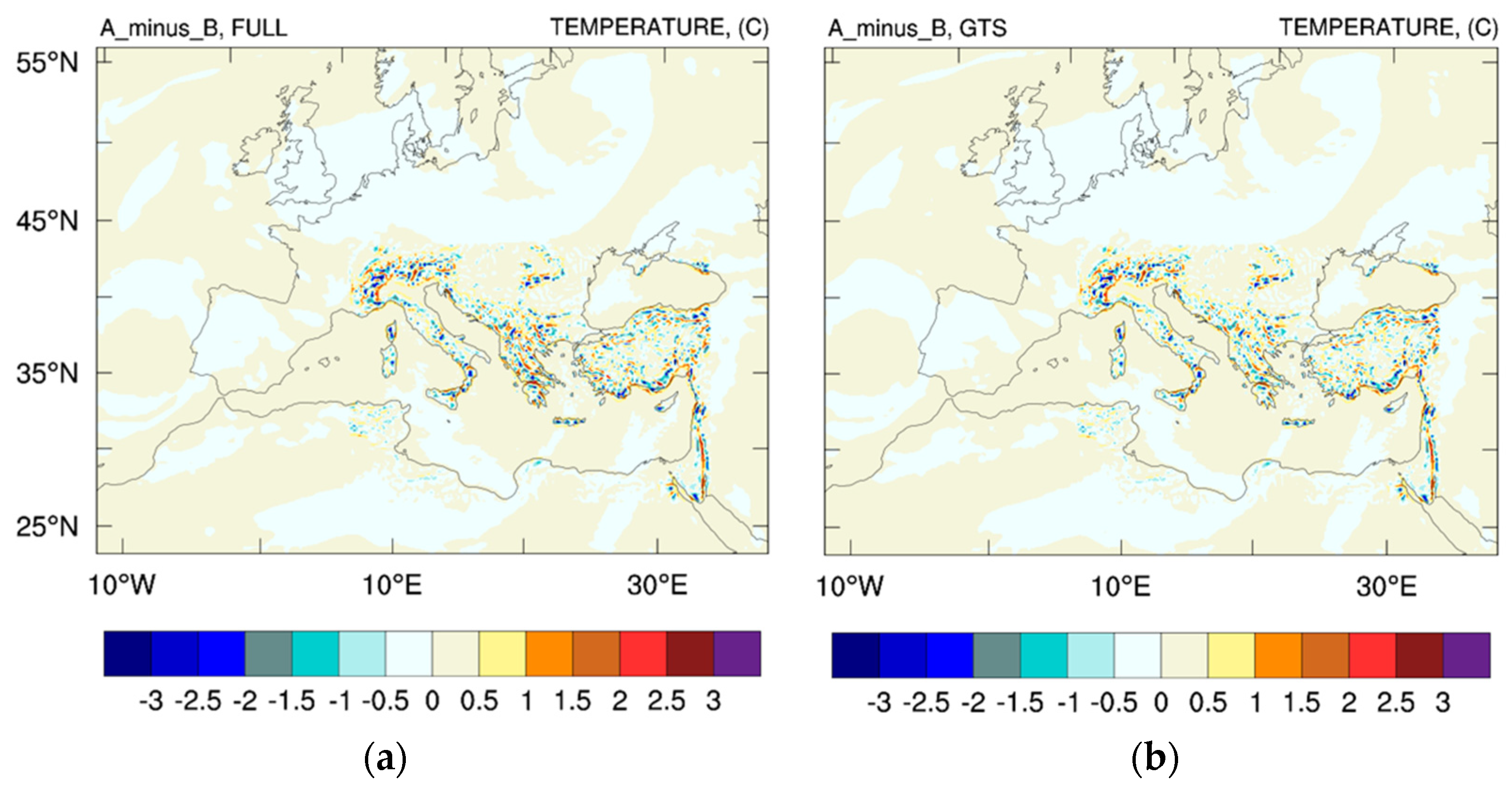
Ianos—Case Study
4. Summary and Discussion
Author Contributions
Funding
Institutional Review Board Statement
Informed Consent Statement
Data Availability Statement
Acknowledgments
Conflicts of Interest
References
- Kalnay, E. Atmospheric Modeling, Data Assimilation and Predictability; Cambridge University Press: Cambridge, UK, 2013. [Google Scholar]
- Ban, J.; Liu, Z.; Zhang, X.; Huang, X.Y.; Wang, H. Precipitation data assimilation in WRFDA 4D-Var: Implementation and application to convection-permitting forecasts over United States. Tellus A Dyn. Meteorol. Oceanogr. 2017, 69, 1368310. [Google Scholar] [CrossRef] [Green Version]
- Lopez, P. Direct 4D-Var assimilation of NCEP stage IV radar and gauge precipitation data at ECMWF. Mon. Weather. Rev. 2011, 139, 2098–2116. [Google Scholar] [CrossRef]
- Yi, L.; Zhang, W.; Wang, K. Evaluation of heavy precipitation simulated by the WRF model using 4D-Var data assimilation with TRMM 3B42 and GPM IMERG over the Huaihe River Basin, China. Remote Sens. 2018, 10, 646. [Google Scholar] [CrossRef] [Green Version]
- Wang, J.; Xu, Y.; Yang, L.; Wang, Q.; Yuan, J.; Wang, Y. Data assimilation of high-resolution satellite rainfall product improves rainfall simulation associated with landfalling tropical cyclones in the Yangtze river Delta. Remote Sens. 2020, 12, 276. [Google Scholar] [CrossRef] [Green Version]
- Flaounas, E.; Davolio, S.; Raveh-Rubin, S.; Pantillon, F.; Miglietta, M.M.; Gaertner, M.A.; Hatzaki, M.; Homar, V.; Khodayar, S.; Korres, G.; et al. Mediterranean cyclones: Current knowledge and open questions on dynamics, prediction, climatology and impacts. Weather. Clim. Dyn. 2022, 3, 173–208. [Google Scholar] [CrossRef]
- Cavicchia, L.; von Storch, H.; Gualdi, S. A long-term climatology of medicanes. Clim. Dyn. 2014, 43, 1183–1195. [Google Scholar] [CrossRef]
- Miglietta, M.M. Mediterranean Tropical-Like Cyclones (Medicanes). Atmosphere 2019, 10, 206. [Google Scholar] [CrossRef] [Green Version]
- Pytharoulis, I.; Kartsios, S.; Tegoulias, I.; Feidas, H.; Miglietta, M.; Matsangouras, I.; Karacostas, T. Sensitivity of a Mediterranean Tropical-Like Cyclone to Physical Parameterizations. Atmosphere 2018, 9, 436. [Google Scholar] [CrossRef] [Green Version]
- Ragone, F.; Mariotti, M.; Parodi, A.; Von Hardenberg, J.; Pasquero, C. A Climatological Study of Western Mediterranean Medicanes in Numerical Simulations with Explicit and Parameterized Convection. Atmosphere 2018, 9, 397. [Google Scholar] [CrossRef] [Green Version]
- Ricchi, A.; Miglietta, M.M.; Barbariol, F.; Benetazzo, A.; Bergamasco, A.; Bonaldo, D.; Cassardo, C.; Falcieri, F.M.; Modugno, G.; Russo, G.A.; et al. Sensitivity of a Mediterranean tropical-like cyclone to different model configurations and coupling strategies. Atmosphere 2017, 8, 92. [Google Scholar] [CrossRef]
- Jansa, A.; Arbogast, P.; Doerenbecher, A.; Garcies, L.; Genoves, A.; Homar, V.; Klink, S.; Richardson, D.; Sahin, C. A new approach to sensitivity climatologies: The DTS-MEDEX-2009 campaign. Nat. Hazards Earth Syst. Sci. 2011, 11, 2381–2390. [Google Scholar] [CrossRef]
- Garcies, L.; Homar, V. Are current sensitivity products sufficiently informative in targeting campaigns? A DTS-MEDEX-2009 case study: Testing DTS-MEDEX-2009 Sensitivity Products. Q. J. Roy. Meteorol. Soc. 2014, 140, 525–538. [Google Scholar] [CrossRef]
- Carrió, D.S.; Homar, V. Potential of sequential EnKF for the short-range pre-diction of a maritime severe weather event. Atmos. Res. 2016, 178–179, 426–444. [Google Scholar] [CrossRef]
- Carrió, D.S. Challenges assessing the effect of AMVs to improve the predictability of a medicane weather event using the EnKF. Storm-scale analysis and short-range forecast. Nat. Hazards Earth Syst. Sci. Discuss. 2022; 1–37, preprint. [Google Scholar]
- Carrió, D.S.; Homar, V.; Wheatley, D.M. Potential of an EnKF Storm-Scale Data Assimilation System Over Sparse Observation Regions with Complex Orography. Atmos. Res. 2019, 216, 186–206. [Google Scholar] [CrossRef]
- Lagouvardos, K.; Kotroni, V.; Defer, E.; Bousquet, O. Study of a heavy precipitation event over southern France, in the frame of HYMEX project: Ob-servational analysis and model results using assimilation of lightning. Atmos. Res. 2013, 134, 45–55. [Google Scholar] [CrossRef]
- Torcasio, R.C.; Federico, S.; Comellas Prat, A.; Panegrossi, G.; D’Adderio, L.P.; Dietrich, S. Impact of Lightning Data Assimilation on the Short-Term Precipitation Forecast over the Central Mediterranean Sea. Remote Sens. 2021, 13, 682. [Google Scholar] [CrossRef]
- Tiesi, A.; Pucillo, A.; Bonaldo, D.; Ricchi, A.; Carniel, S.; Miglietta, M.M. Initialization of WRF Model Simulations with Sentinel-1 Wind Speed for Severe Weather Events. Front. Mar. Sci. 2021, 8, 573489. [Google Scholar] [CrossRef]
- Giannaros, C.; Kotroni, V.; Lagouvardos, K.; Giannaros, T.M.; Pikridas, C. Assessing the Impact of GNSS ZTD Data Assimilation into the WRF Modeling System during High-Impact Rainfall Events over Greece. Remote Sens. 2020, 12, 383. [Google Scholar] [CrossRef] [Green Version]
- Lagouvardos, K.; Karagiannidis, A.; Dafis, S.; Kalimeris, A.; Kotroni, V. Ianos—A hurricane in the Mediterranean. Bull. Am. Meteorol. Soc. 2022, 103, E1621–E1636. [Google Scholar] [CrossRef]
- Global Forecasting System (GFS). Available online: https://www.ncei.noaa.gov/access/metadata/landing-page/bin/iso?id=gov.noaa.ncdc:C00634 (accessed on 7 October 2022).
- NCEP Products Inventory, Sea Surface Temperature (SST) Models. Available online: https://www.nco.ncep.noaa.gov/pmb/products/sst/ (accessed on 23 August 2022).
- Skamarock, W.; Klemp, J.; Dudhia, J.; Gill, D.; Liu, Z.; Berner, J.; Huang, X.-Y.; Wang, W.; Powers, J.G.; Duda, M.G.; et al. A Description of the Advanced Research WRF Version 4; NCAR Tech: Boulder, CO, USA, 2019; Note NCAR/TN-556+STR. [Google Scholar] [CrossRef]
- Hong, S.Y.; Noh, Y.; Dudhia, J. A new vertical diffusion package with an explicit treatment of entrainment processes. Mon. Weather. Rev. 2006, 134, 2318–2341. [Google Scholar] [CrossRef] [Green Version]
- Niu, G.Y.; Yang, Z.L.; Mitchell, K.E.; Chen, F.; Ek, M.B.; Barlage, M.; Xia, Y.; Kumar, A.; Manning, K.; Niyogi, D.; et al. The community Noah land surface model with multiparameterization options (Noah-MP): 1. Model description and evaluation with local-scale measurements. J. Geophys. Res. Atmos. 2011, 116. [Google Scholar] [CrossRef] [Green Version]
- Jimenez, P.A.; Dudhia, J.; Gonzalez–Rouco, J.F.; Navarro, J.; Montavez, J.P.; Garcia–Bustamante, E. A revised scheme for the WRF surface layer formulation. Mon. Wea. Rev. 2012, 140, 898–918. [Google Scholar] [CrossRef] [Green Version]
- Iacono, M.J.; Delamere, J.S.; Mlawer, E.J.; Shephard, M.W.; Clough, S.A.; Collins, W.D. Radiative forcing by long–lived greenhouse gases: Calculations with the AER radiative transfer models. J. Geophys. Res. 2008, 113, D13103. [Google Scholar] [CrossRef]
- Kain, J.S. The Kain–Fritsch convective parameterization: An update. J. Appl. Meteor. 2004, 43, 170–181. [Google Scholar] [CrossRef]
- Development Testbed, Unified Post Processor (UPP). Available online: https://dtcenter.org/community-code/unified-post-processor-upp (accessed on 23 August 2022).
- Development Testbed, Model Evaluation Tools (MET). Available online: https://dtcenter.org/community-code/model-evaluation-tools-met (accessed on 23 August 2022).
- Docker Hub Page for the Official Image of MET. Available online: https://hub.docker.com/r/dtcenter/met (accessed on 23 August 2022).
- Meteorological Assimilation Data Ingest System. Available online: https://madis.ncep.noaa.gov/ (accessed on 7 October 2022).
- NASA Official Website for the Integrated Multi-SatellitE Retrievals for GPM. Available online: https://gpm.nasa.gov/data/imerg (accessed on 23 August 2022).
- ERA5-Land Data Page on Climate Data Store. Available online: https://cds.climate.copernicus.eu/cdsapp#!/dataset/reanalysis-era5-land?tab=overview (accessed on 23 August 2022).
- MET Software Documentation Concerning the Interpolation/matcing Methods Applied. Available online: https://met.readthedocs.io/en/latest/Users_Guide/point-stat.html?highlight=distance%20weighted%20mean%20#interpolation-matching-methods (accessed on 26 September 2022).
- Hu, X.-M.; Klein, P.M.; Xue, M. Evaluation of the updated YSU planetary boundary layer scheme within WRF for wind resource and air quality assessments. J. Geophys. Res. Atmos. 2013, 118, 10490–10505. [Google Scholar] [CrossRef]


Publisher’s Note: MDPI stays neutral with regard to jurisdictional claims in published maps and institutional affiliations. |
© 2022 by the authors. Licensee MDPI, Basel, Switzerland. This article is an open access article distributed under the terms and conditions of the Creative Commons Attribution (CC BY) license (https://creativecommons.org/licenses/by/4.0/).
Share and Cite
Vourlioti, P.; Mamouka, T.; Agrafiotis, A.; Kotsopoulos, S. Medicane Ianos: 4D-Var Data Assimilation of Surface and Satellite Observations into the Numerical Weather Prediction Model WRF. Atmosphere 2022, 13, 1683. https://doi.org/10.3390/atmos13101683
Vourlioti P, Mamouka T, Agrafiotis A, Kotsopoulos S. Medicane Ianos: 4D-Var Data Assimilation of Surface and Satellite Observations into the Numerical Weather Prediction Model WRF. Atmosphere. 2022; 13(10):1683. https://doi.org/10.3390/atmos13101683
Chicago/Turabian StyleVourlioti, Paraskevi, Theano Mamouka, Apostolos Agrafiotis, and Stylianos Kotsopoulos. 2022. "Medicane Ianos: 4D-Var Data Assimilation of Surface and Satellite Observations into the Numerical Weather Prediction Model WRF" Atmosphere 13, no. 10: 1683. https://doi.org/10.3390/atmos13101683