A Practical Approach for Determining Multi-Dimensional Spatial Rainfall Scaling Relations Using High-Resolution Time–Height Doppler Data from a Single Mobile Vertical Pointing Radar

Abstract

The rescaling of rainfall requires measurements of rainfall rates over many dimensions. This paper develops one approach using 10 m vertical spatial observations of the Doppler spectra of falling rain every 10 s over intervals varying from 15 up to 41 min in two different locations and in two different years using two different micro-rain radars (MRR). The transformation of the temporal domain into spatial observations uses the Taylor “frozen” turbulence hypothesis to estimate an average advection speed over an entire observation interval. Thus, when no other advection estimates are possible, this paper offers a new approach for estimating the appropriate frozen turbulence advection speed by minimizing power spectral differences between the ensemble of purely spatial radial power spectra observed at all times in the vertical and those using the ensemble of temporal spectra at all heights to yield statistically reliable scaling relations. Thus, it is likely that MRR and other vertically pointing Doppler radars may often help to obviate the need for expensive and immobile large networks of instruments in order to determine such scaling relations but not the need of those radars for surveillance.

1. Introduction

Scaling is an essential feature of many phenomena ranging from those of cosmology to those of quantum physics [1]. Many human activities, from the stock market [2] to ecology [3] and many more, are also impacted by scaling. The science of scaling “helps reveal what factors determine … the …level of impact in a different place, in a different situation, and with a different population. How big is it? How long does it last? These are [some of] the most basic questions a scientist can ask.” ([4], p. 107).

With respect to direct physical impacts on mankind, this is especially true for rainfall. Moreover, it has been shown [5] that the temporal and spatial structures of rain are not equivalent because they are orthogonal dimensions but also in part because the unknown advection of the rain affects the temporal observations. Furthermore, until recently [6], studies of spatial scaling have all been confined to the surface. However, the vertical dimension retains particular relevance not only with respect to the evolution of rain but also because observations at the surface are only an ambiguous expression of what is happening aloft. That is, the structure and statistical characteristic above the ground will not necessarily be unambiguously reflected on the surface because of storm motion and boundary layer surface winds. Furthermore, rain evolves as it descends, altering what is seen aloft from what may appear at the ground. Thus, in general, the physical/statistical structure and scales at the surface will likely be somewhat different from those observed in the vertical [6]. Thus, combining observations in both dimensions may yield more generally applicable results.

However, whether in the vertical or horizontal, the different scales of rainfall are obvious even to the most casual observer. Specifically, proceeding from the smallest scales we have, soil erosion (e.g., [7]) and agricultural run-off and pollution, up to larger scales which influence flash flooding and urban water management (e.g., [8]), and finally up to the largest scales (e.g., [9]) which play a major role in the world climate. Consequently, downscaling—going from the large dimensions of, for example, a numerical model, a measurement using a spaceborne instrument [10], or even a coarse resolution radar measurement down to smaller scales [11]—and upscaling—going from essentially point measurements, such as using a rain gauge or disdrometer up to the larger scales just mentioned [12,13]—are both equally important depending upon the situation.

In the literature, there is an assortment of techniques for downscaling, such as the so-called multiplicative cascading method [14,15,16] with improvements proposed by Seed et al. [17]. An alternative approach that reproduces the observed power spectrum uses the observed correlation functions (when valid) or the power spectrum [12,13,18] to downscale observations to smaller domains while maintaining the physical and statistical character of the observed rain. This will be illustrated in Appendix A.

Methods for upscaling, however, are more limited, although a few exist. Some involve smoothing [19] or Kriging of the observations [19,20]. The primary limitation of such techniques is that they are filters of the power spectra [21] leading to a reduction of information as discussed in [22]. A different approach uses the Bayesian components of the rainfall and the observed power spectrum (or correlation function for statistically homogeneous rain) to generate rain over many different scales with the appropriate statistical properties consistent with the observations [12]. This will be briefly mentioned in Appendix A as well with appropriate references for the interested reader to pursue.

Regardless of methodology, however, the statistical properties of the rain must be properly characterized and preserved. In the next sections, we report on improved re-analyses of time–height observations presented in [6] to produce radial power functions for scaling, which more accurately represent the data. In this work, results are presented using micro-rain radar (MRR) vertical-pointing Doppler radar observations in four cases in two different locations using two different radars—three from observations at the NASA Wallop’s Island Virginia facility and the other from measurements collected using the College of Charleston’s MRR radar near Charleston, South Carolina. An example of downscaling using a similar but not identical power law fit is given in an appendix with references to view for upscaling examples.

Time–height data are challenging since in the spatial dimension, power spectra yield the number of waves per unit length, while in the temporal dimension, the power spectra yield the frequency. In order to determine the spatial radial power spectra used to perform the rainfall rescaling. (the power spectrum as a function of distance along any radial) for all directions, the two must be combined [21]. The radial power spectrum is calculated by first computing the 2D horizontal–vertical coordinate system of the original 2D power spectrum using the fft2 routine in Matlab^® and then multiplying by its complex conjugate. This 2D power spectrum of values in (Δz, Δh) coordinates is then converted into 2D polar coordinate system of (Δr, Δθ) values of the power spectrum. Finally, the radial power spectra can then be computed by integrating over all the angles Δθ for each Δr. The first-order standard approach for transforming time to space is to use an average advection velocity for the storm combined with Taylor’s frozen turbulence hypothesis. The frozen turbulence advection velocity is that velocity that transform the turbulence spectra in time to that in space. In one horizontal dimension, the velocity becomes a speed. In past work, this was performed arbitrarily so that the quality of the results was uncertain even if it was “reasonable”. As we show below, there is a much better, more objective approach for better estimating an advection speed consistent with frozen turbulence that involves comparing the independent spatial and advection transformed temporal spectra. This likely differs from an estimate of a storm’s advection velocity based upon the movement of storm features undergoing constant changes since frozen turbulence is not identical to frozen structures. Importantly, under conditions with a proper advection speed, time–height profiles using one radar can offer observations over a large spatial domain when more expensive networks of instruments are not available. This is further developed in the next section.

2. Background

2.1. Basic Considerations

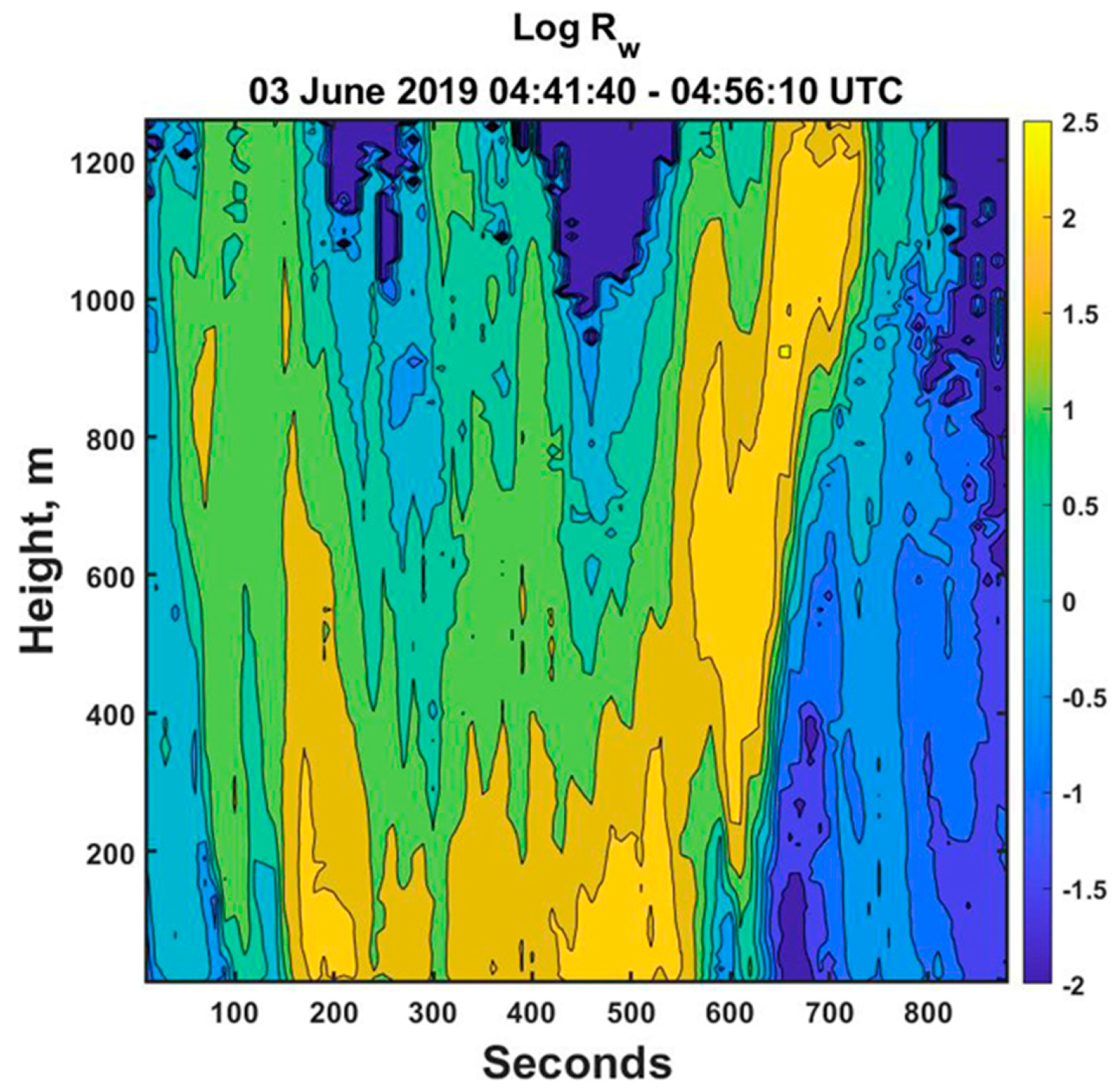
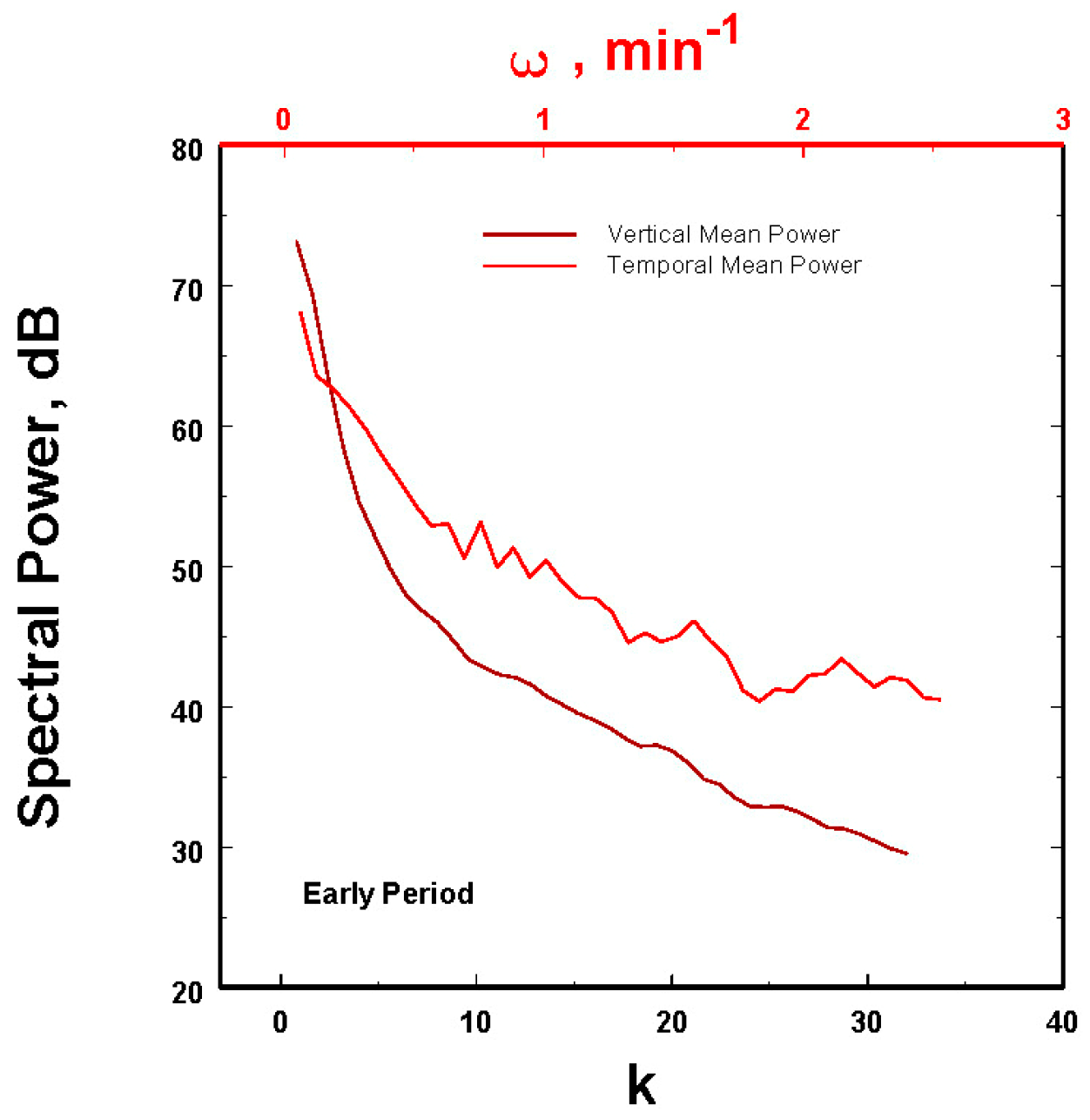
In order to be able to fully scale the rain rate, R, in any spatial direction, it is most useful to have access to the radial power spectra that, in the case of statistically homogeneous rain, can also be transformed into the radial correlation function. (e.g., for a discussion, see [23]. Accomplishing estimates of the rainfall rates at high resolution is a challenging task that is perhaps best addressed using vertical-pointing Doppler radar data in rain. Thus, one of the most potentially useful radars for collecting such observations in a number of different locations and meteorological settings is the micro-rain radar (MRR) described in [24]. This is a lightweight, highly transportable, low-power, vertical-pointing continuous wave radar operating at a frequency of 24.23 GHz.

There are challenges, however. The rainfall rate is calculated from the drop sizes deduced from the Doppler spectra using well-established relations between the fall speed of a drop and its size [25] with the drop concentration determined from the radar backscatter cross-section in relation to drop size for the particular wavelength being used. Both of these quantities (the apparent fall speed and observed radar backscattered power), however, require adjustments. In particular, the observed Doppler velocity is the sum of the true fall speed of the drop and the vertical air motion, which must be removed in order to estimate the correct drop fall speed and size. Similarly, at the wavelength of the MRR instrument, attenuation by the rain can become significant at times depending upon the rain intensity and distance of the sampling bin (range) from the radar. Both of these concerns have been addressed in [6], so an interested reader can refer to that paper for elaboration. Here, we take the deduced rainfall rates from that work for the data mentioned above and use them for further analyses.

The challenge explored in this work is how best to address the fact that space and time are orthogonal dimensions such that a method must be identified in order to combine measurements in each. That is, radar time–height observations are the sequential temporal measurements of the rainfall rate, R, at each sampling bin spatially sequentially in the vertical. For the data used here, data were collected over 10 m depths from about 30 m above the ground up to a height of 1280 m. At each location the Doppler spectra and radar backscattered powers were measured over sequential 10 s sampling periods for each determination of R at each height and time. Over an interval of observations, these data can then be considered in two ways, namely as a sequential ensemble of vertical spatial profiles or, alternatively, as the ensemble of times series of observations at each height. Using the Fourier transform for each of these, one can compute both the ensemble of vertical spatial power spectra and, simultaneously, a different ensemble of the temporal power spectra at each height. As we shall see, this allows for a better estimation of the frozen turbulence advection speed.

2.2. An Example

To make this all more concrete, we initially consider the opening 950 s of observations for a line of intense convective rainstorms that passed over the NASA Wallop’s Island Flight Facility on 3 June 2019, as illustrated in Figure 1.

Hence, over these 900 s of observations collected every 10 s, we obtained 90–128 rainfall rate estimates in height from the Doppler measurements. Therefore, for each of these 10 s periods, we could compute the power of the rainfall rate spectrum as a function of height. Furthermore, corresponding to each height, there would be 90 temporal observations of the rainfall rates. Thus, we could compute the power of the rainfall rate spectrum in time at each height. That is, these data allowed for the generation of 90 power–rainfall rate–distance spectra corresponding to the 90 10 s intervals and 128 power–rainfall rate spectra in time corresponding to each 10 m separation in height. However, since we are most interested in the average properties of all these data, all the power spectra were averaged in their own dimensions to yield the mean power–rainfall rate–height and temporal spectra, as illustrated in Figure 2.

The two spectra are clearly different. This is, of course, not surprising since one is necessarily expressed as a temporal frequency, while the other is written in terms of the wave number. If one desires to have a radial power spectrum for spatial scaling, is there a way to combine these two observations taken along two different orthogonal axes? To express it slightly differently, can the frequency ω be transformed into reasonable estimates of k? The assumption when trying to make this transformation is that the temporal observations are considering approximately the same phenomenon but along a different axis, i.e., ω = V_a × k where V_a is defined to be the mean advection speed, providing that it can be determined.

While the motion of the rain is undoubtedly complicated, moving at different speeds at different locations and times, the simplest first approximation is to use the Taylor hypothesis that the rain is moving as a whole at V_a so that the observed frequencies are truly the consequence of the mean motion of the spatial structures. Can V_a be determined?

The answer is yes if a speed can be found that transforms most of the temporal power spectra into something that more closely approximates the observed spatial power spectra. To see how this may work, the temporal power spectra in Figure 2 were transformed from ω to k using a range of possible advection velocities. That is, for a particular spatial wavelength, in the temporal domain, the velocity can be viewed as a stretching of the wavelength. Consequently, the transformed wave number will be smaller than in the spatial domain. 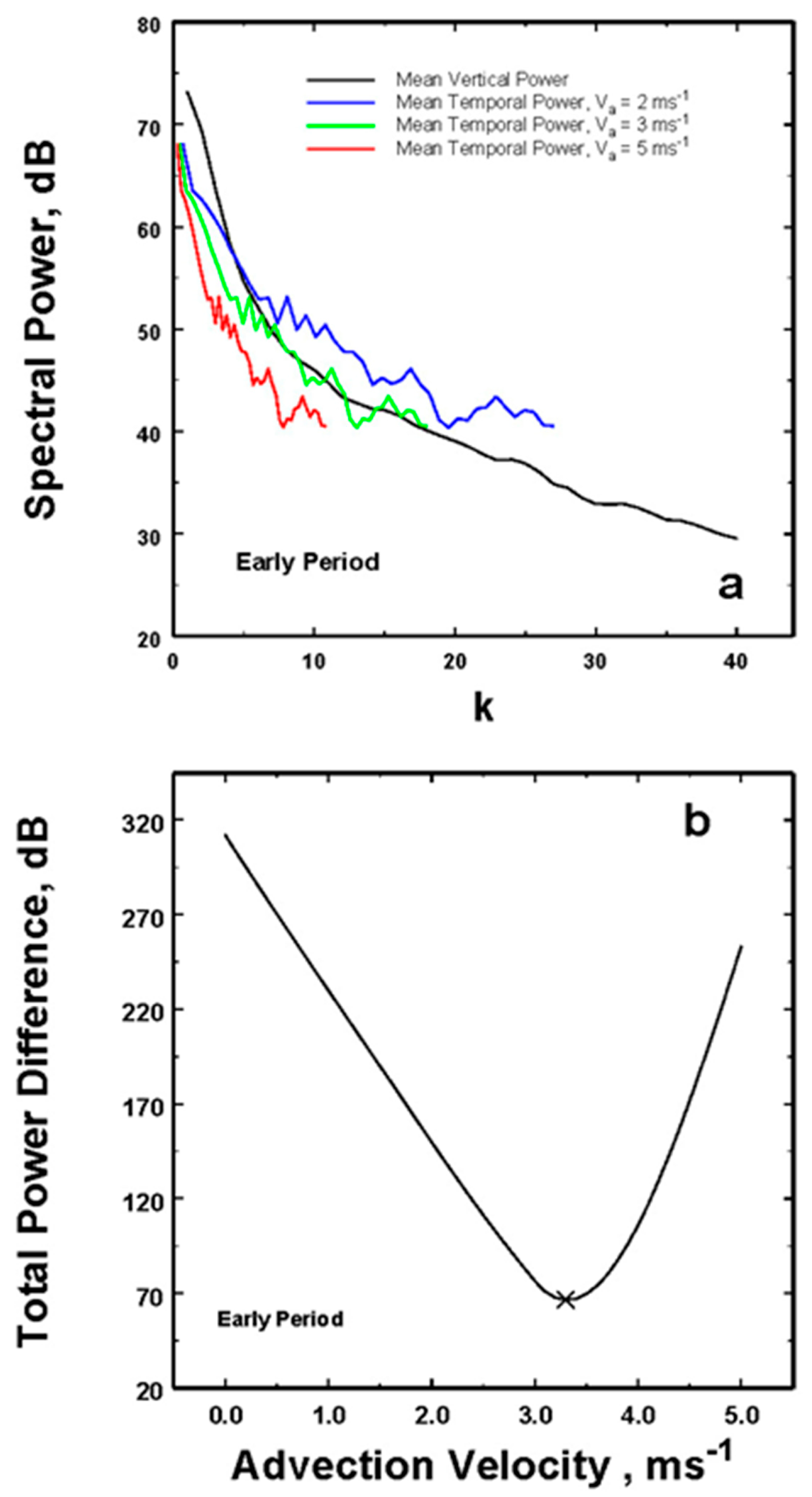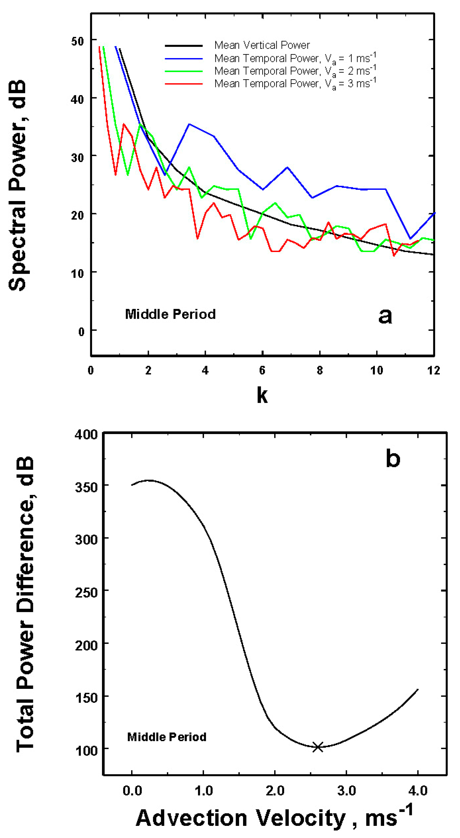Another way to consider this is that if the characteristic spatial domain size is while the total temporal interval of observations is T, then the equivalent spatial domain size corresponding to T would be = V_a × T, where V_a is a characteristic advection speed. For a fixed spatial wavelength, λ, then there would be k = L/λ number of wavelengths in the spatial domain, but there would be k_ω = /λ such wavelengths in the velocity transformed from the temporal to spatial domain. Hence, the k_ω associated with that λ would be much larger than k, i.e., k_ω = ( /L) × k. Thus, in order to match the two wavenumbers so that they correspond to the same λ, k_ω must be multiplied by L/ , as illustrated in Figure 3a for this example.

Other examples will be shown below as well, but this velocity also allows us to rescale all the spatial data in Figure 1, as shown in Figure 4, thereby reducing the overly exaggerated appearance of the vertical structures.

3. Further Data Analyses

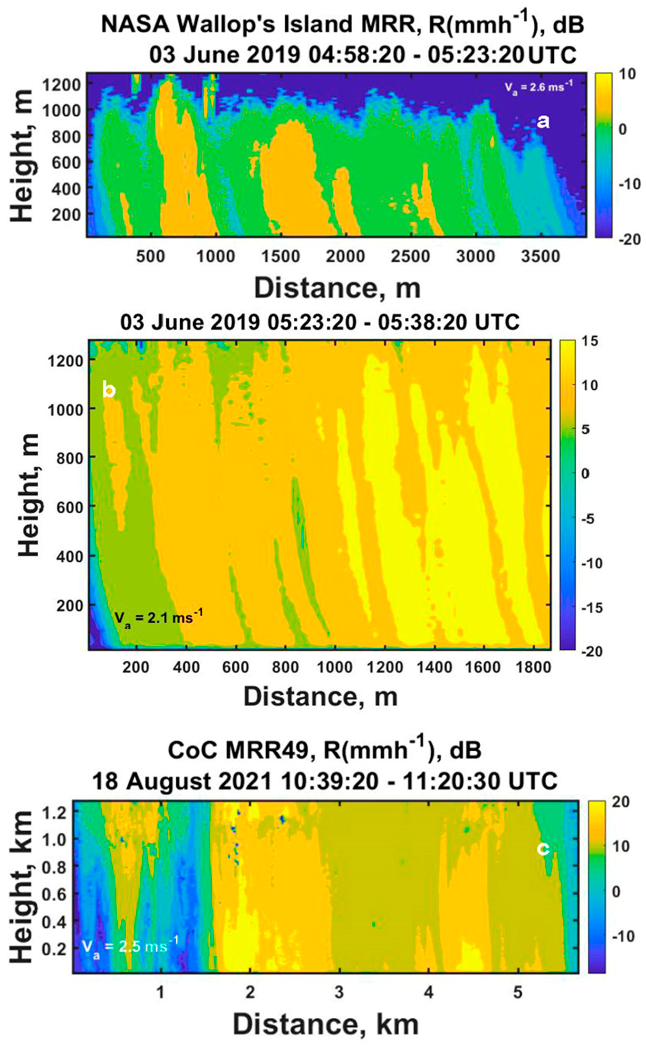
3.1. Three More Cases

Before computing the associated radial power spectrum for these specific data, however, we next consider the other three sets of measurements used in this study. This will then allow direct comparisons between all of the radial power spectra that could be used for upscaling or downscaling of these observations as illustrated in the appendix. To that end, for convenience, we begin in Figure 5 by first simply displaying the additional data to be processed using illustrations in a previous paper [6]. The first two are a continuation of the data presented above, but for a middle period (Figure 5a), a later period (Figure 5b), and finally for a different set of measurements using a different MRR at the College of Charleston (CoC data) gathered in a storm in August, 2021 (Figure 5c).

Beginning with the middle period data, the power spectra are plotted in Figure 6a with the determination of the optimum V_a shown in Figure 6b. For these data, the optimum advection speed of 2.6 ms⁻¹ is about 0.7 ms⁻¹ less than that for the line of storms moving over the radar in the previous early data set.

For the later period, a similar plot is shown in Figure 7. At this later time, the optimal advection speed is even slightly smaller at 2.1 ms⁻¹, thus showing a persistent decrease in time over the 40 min period of these observations.

Lastly are the College of Charleston (CoC) data through an ordinary but significant South Carolina summer thunderstorm, with results illustrated in Figure 8. Once again, the advection speed is reasonable at about 2.4 ms^−1.

With these advection speeds and for completeness, we can then replot the time-height profiles as height distance profiles for these data (as was done in Figure 4), as illustrated in Figure 9. These most likely represent the actual spatial structures that we can now analyze to derive the spatial radial power spectra for rainfall scaling for each set of data separately.

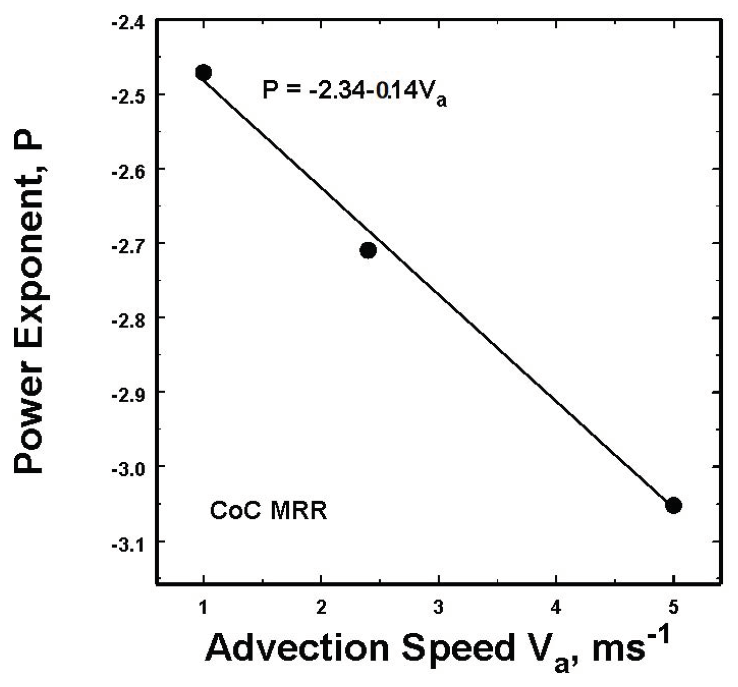
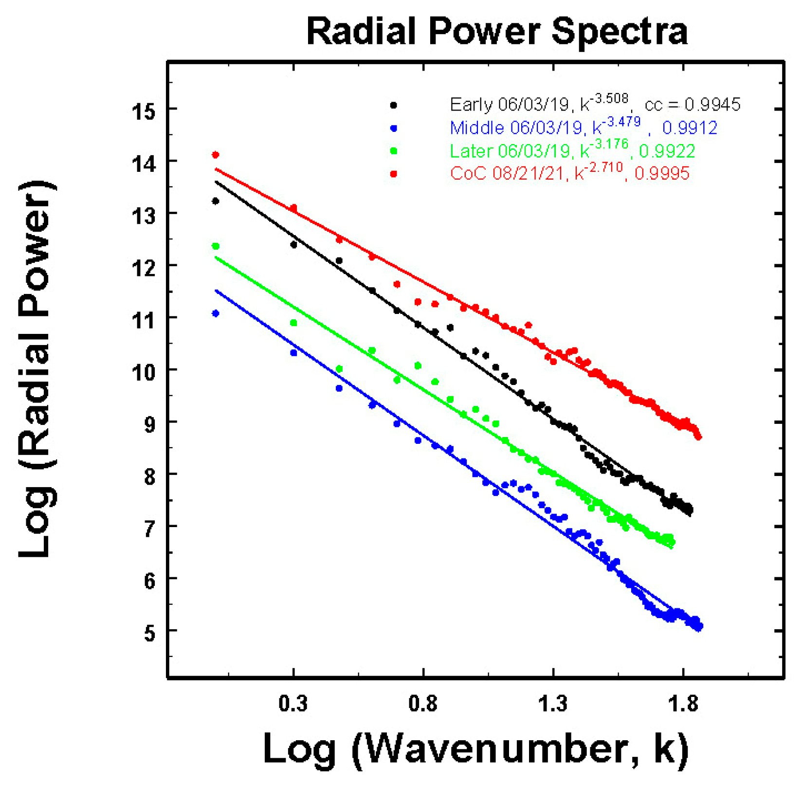
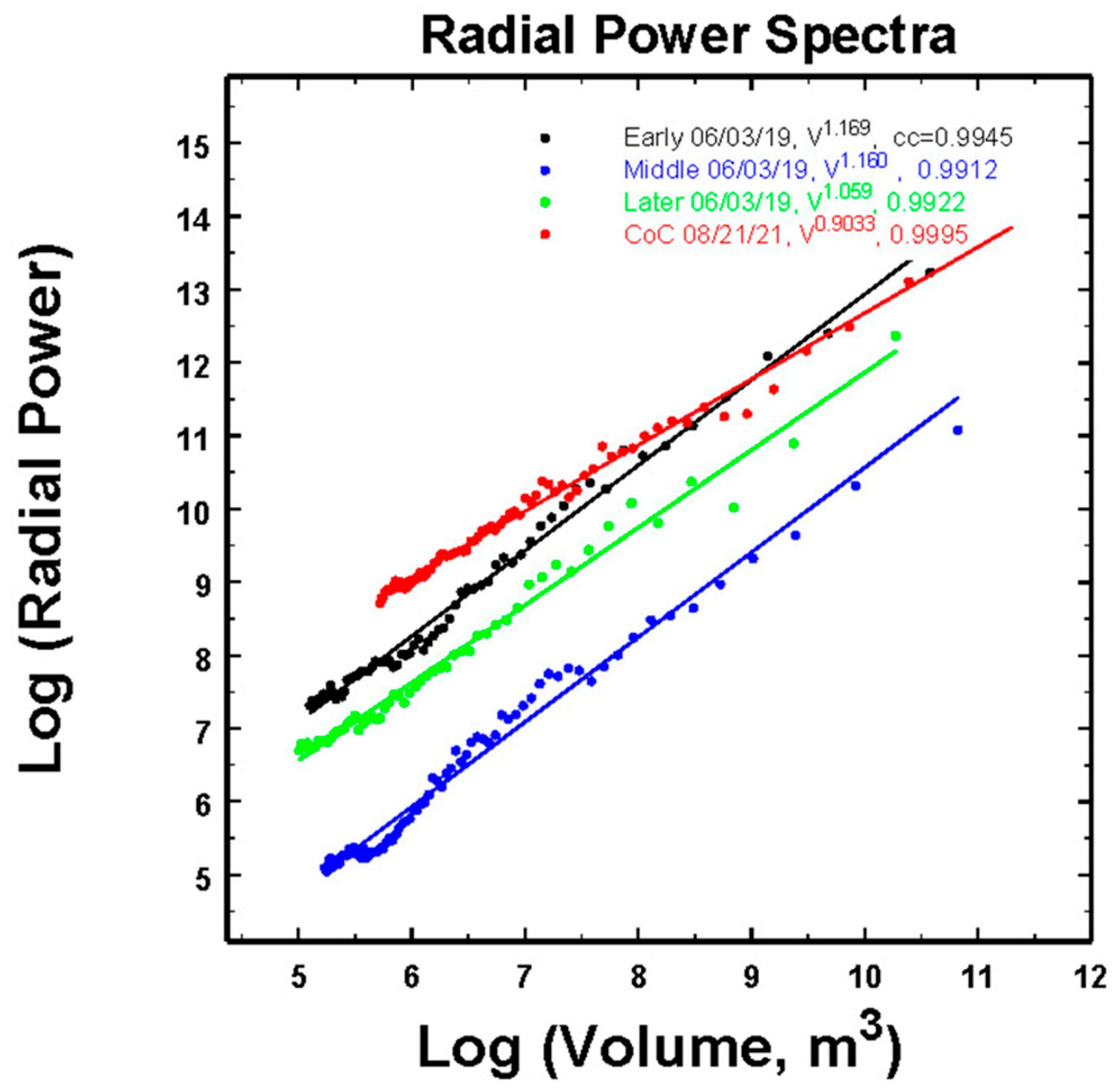
3.2. The Radial Power Spectra for Use in Rescaling

With these estimates of advection velocities, there are then only spatial variables in both the vertical (z) and horizontal (h) directions, so the one-dimensional radial power spectra can be computed for all of these data sets for subsequent use in rescaling out to the maximum range $Rn{g}_{max}=\sqrt{z^2+h^2}$. As explained in [26] but repeated here for readability, this is accomplished by first computing the 2D horizontal–vertical coordinate system of the original 2D power spectrum using the fft2 routine in Matlab^® and then multiplying by its complex conjugate. This 2D power spectrum of values in (Δz, Δh) coordinates is then converted into a 2D polar coordinate system of (Δr, Δθ) values of the power spectrum. Finally, the radial spectra can then be computed by integrating over all the angles Δθ for each Δr.

Before displaying the results, it is important to recognize the value of using the best estimate of the advection velocities as indicated for the CoC data in Figure 10. This is likely important for the other data in this study as well. Thus, in the previous work, (Figure 9 of [26]) which calculated erroneously by assuming the incorrect V_a = 1 ms⁻¹, the values of the slopes only ranged from −2.47 to −2.74, while those below in Figure 11—calculated using the best estimates of V_a—fall over a greater range of slopes between −2.71 and −3.51.

However, while the maximum differences in slopes in Figure 11 is about 0.8, this decreases to about 0.27 after first noting that these relations can all be scaled to the volume (Figure 12). Here, the volume is calculated from the expression:

$$Log\left(V_k\right)=3Log\left(Rn{g}_{max}\right)-3Log\left(k\right)$$

(1)

where V_k is the volume associated with wave number k arising for each length scale defined by a L = Rng_max/k and V_k = L³ and a maximum length of Rng_max defined above. In this transform, the slopes now vary over a much narrower range of values from −0.9 to −1.17, while the minima in spectral powers at (k = 1) are indicative of the overall mean rainfall intensity (29.7, 25.6, 21.5, 1.65 mm h⁻¹ for the CoC, early, later, and middle data sets, respectively). Interestingly, under conditions with a proper advection speed, time–height profiles using one radar offer the potential for observations over large spatial domains when more expensive networks of many instruments are not available.

4. Summary of Results

This work explored, in detail, an option for using time–height Doppler radar spectra for estimating rainfall rate over a large spatial domain in order to compute radial power spectra for any subsequent rescaling of new input observations or numerical model outputs. Using the rainfall rates determined through an earlier analyses of these data [6], a method was found to convert the temporal observations into spatially equivalent measurements using the concept of a mean advection speed so that the temporal frequency power fluctuations could be interpreted as the temporal reflection of moving spatial structures, thus satisfying the meaning of frozen turbulence. Moreover, under the assumption of approximate spatial isotropy, an optimal physically based advection speed could be estimated by comparing the spatially transformed temporal power spectra to the purely spatial power in the vertical. In each set of data, a unique frozen turbulence advection speed was found such that the total differences between the spatial power spectra and the transformed temporal power spectra were minimized. Using these advection speeds, all of the time–height observations were then converted into vertical and horizontal spatial data, which were subsequently used to compute the spatial radial power spectra for all the different sets of data. In the appendix, an example is provided of how such radial spectra can be used to downscale a uniform mean rainfall rate over a one-kilometer area into a set of statistically homogeneous “data” with the structures of various dimensions consistent with the radial power spectrum.

A significant advantage illustrated by these results is that such data from a single works of instruments in order to determine radial power spectra for rescaling, and it provides observations in the vertical not otherwise possible to obtain. Thus, it opens up the possibility that such measurements may be made in locations where such networks of instrumentation may not even be possible or feasible but also when mobility is important for collecting observations in widely varying meteorological situations.

References

1. Rauscher, E.A.; Hurtak, J.J.; Hurtak, D.E. Universal Scaling Laws in Quantum Theory and Cosmology. In The Physics of Reality: Space, Time, Matter, Cosmos; WORLD SCIENTIFIC: London, UK, 2013; pp. 376–387. [Google Scholar]
2. Walter, C. Research of Scaling Law on Stock Market Variations. In Scaling, Fractals and Wavelets; Abry, P., Gonalves, P., Vhel, J.L., Eds.; ISTE: London, UK, 2009; pp. 437–464. ISBN 978-0-470-61156-2. [Google Scholar]
3. Ellison, A.M.; Gotelli, N.J. Scaling in Ecology with a Model System; Monographs in Population Biology; Princeton University Press: Princeton, NJ, USA, 2021; ISBN 978-0-691-17270-5. [Google Scholar]
4. Gleick, J. Chaos: Making a New Science, 20th Anniversary ed.; Penguin Books: New York, NY, USA, 2008; ISBN 978-0-14-311345-4. [Google Scholar]
5. Jameson, A.R.; Larsen, M.L.; Kostinski, A.B. Disdrometer Network Observations of Finescale Spatial–Temporal Clustering in Rain. J. Atmos. Sci. 2014, 72, 1648–1666. [Google Scholar] [CrossRef] [Green Version]
6. Jameson, A.R.; Larsen, M.L.; Wolff, D.B. Improved Estimates of the Vertical Structures of Rain Using Single Frequency Doppler Radars. Atmosphere 2021, 12, 699. [Google Scholar] [CrossRef]
7. Piacentini, T.; Galli, A.; Marsala, V.; Miccadei, E. Analysis of Soil Erosion Induced by Heavy Rainfall: A Case Study from the NE Abruzzo Hills Area in Central Italy. Water 2018, 10, 1314. [Google Scholar] [CrossRef] [Green Version]
8. Cristiano, E.; ten Veldhuis, M.-C.; van de Giesen, N. Spatial and Temporal Variability of Rainfall and Their Effects on Hydrological Response in Urban Areas – a Review. Hydrol. Earth Syst. Sci. 2017, 21, 3859–3878. [Google Scholar] [CrossRef] [Green Version]
9. Hatsuzuka, D.; Sato, T.; Higuchi, Y. Sharp Rises in Large-Scale, Long-Duration Precipitation Extremes with Higher Temperatures over Japan. Npj Clim. Atmospheric Sci. 2021, 4, 29. [Google Scholar] [CrossRef]
10. Zorzetto, E.; Marani, M. Downscaling of Rainfall Extremes From Satellite Observations. Water Resour. Res. 2019, 55, 156–174. [Google Scholar] [CrossRef] [Green Version]
11. Chen, H.; Qin, H.; Dai, Y. FC-ZSM: Spatiotemporal Downscaling of Rain Radar Data Using a Feature Constrained Zooming Slow-Mo Network. Front. Earth Sci. 2022, 10, 887842. [Google Scholar] [CrossRef]
12. Jameson, A.R. A Bayesian Method for Upsizing Single Disdrometer Drop Size Counts for Rain Physics Studies and Areal Applications. IEEE Trans. Geosci. Remote Sens. 2015, 53, 335–343. [Google Scholar] [CrossRef]
13. Das, S.; Jameson, A.R. Site Diversity Prediction at a Tropical Location From Single-Site Rain Measurements Using a Bayesian Technique. Radio Sci. 2018. [Google Scholar] [CrossRef]
14. Lovejoy, S.; Mandelbrot, B.B. Fractal Properties of Rain, and a Fractal Model. Tellus A 1985, 37A, 209–232. [Google Scholar] [CrossRef]
15. Lovejoy, S.; Schertzer, D. Multifractals, Universality Classes and Satellite and Radar Measurements of Cloud and Rain Fields. J. Geophys. Res. Atmos. 1990, 95, 2021–2034. [Google Scholar] [CrossRef]
16. Venugopal, V.; Foufoula-Georgiou, E.; Sapozhnikov, V. A Space-Time Downscaling Model for Rainfall. J. Geophys. Res. 1999, 104, 19705. [Google Scholar] [CrossRef]
17. Seed, A.W.; Srikanthan, R.; Menabde, M. A Space and Time Model for Design Storm Rainfall. J. Geophys. Res. Atmos. 1999, 104, 31623–31630. [Google Scholar] [CrossRef]
18. Jameson, A.R.; Heymsfield, A.J. Bayesian Upscaling of Aircraft Ice Measurements to Two-Dimensional Domains for Large-Scale Applications. Meteorol. Atmos. Phys. 2014, 123, 93–103. [Google Scholar] [CrossRef] [Green Version]
19. Frei, C.; Schar, C. A Precipitation Climatology of the Alps from High-Resolution Rain-Gauge Observations. Int. J. Climatol. 1998, 18, 873–900. [Google Scholar] [CrossRef]
20. Rubel, F.; Hantel, M. BALTEX 1/6-Degree Daily Precipitation Climatology 1996-1998. Meteorol. Atmos. Phys. 2001, 77, 155–166. [Google Scholar] [CrossRef]
21. Jameson, A.R. Spatial and Temporal Network Sampling Effects on the Correlation and Variance Structures of Rain Observations. J. Hydrometeorol. 2017, 18, 187–196. [Google Scholar] [CrossRef]
22. Ahrens, B.; Beck, A. On Upscaling of Rain-Gauge Data for Evaluating Numerical Weather Forecasts. Meteorol. Atmos. Phys. 2008, 99, 155–167. [Google Scholar] [CrossRef] [Green Version]
23. Jameson, A.R. On the Importance of Statistical Homogeneity to the Scaling of Rain. J. Atmos. Ocean. Technol. 2019, 36, 1063–1078. [Google Scholar] [CrossRef]
24. Löffler-Mang, M.; Kunz, M.; Schmid, W. On the Performance of a Low-Cost K-Band Doppler Radar for Quantitative Rain Measurements. J. Atmos. Ocean. Technol. 1999, 16, 379–387. [Google Scholar] [CrossRef]
25. Gunn, R.; Kinzer, G.D. The Terminal Velocity OffallL for Water Droplets in Stagnant Air. J. Meteorol. 1949, 6, 243–248. [Google Scholar] [CrossRef]
26. Jameson, A.R.; Larsen, M.L. Preliminary Statistical Characterizations of the Lowest Kilometer Time–Height Profiles of Rainfall Rate Using a Vertically Pointing Radar. Atmosphere 2022, 13, 635. [Google Scholar] [CrossRef]
27. Wiener, N. Generalized Harmonic Analysis. Acta Math. 1930, 55, 117–258. [Google Scholar] [CrossRef]
28. Khintchine, A. Korrelationstheorie der stationaren stochastischen Prozesse. Math. Ann. 1934, 109, 604–615. [Google Scholar] [CrossRef]
29. Johnson, G.E. Constructions of Particular Random Processes. Proc. IEEE 1994, 82, 270–285. [Google Scholar] [CrossRef]
30. Jameson, A.R.; Kostinski, A.B. Fluctuation Properties of Precipitation. Part V: Distribution of Rain Rates—Theory and Observations in Clustered Rain. J. Atmos. Sci. 1999, 56, 3920–3932. [Google Scholar] [CrossRef]
31. Nelsen, R.B. An Introduction to Copulas, 2nd ed.; Springer Series in Statistics; Springer: New York, NY, USA, 2006; ISBN 978-0-387-28659-4. [Google Scholar]
Figure 1. Time–height profile of the logarithm of the rainfall rate as derived in [6] for the so-called early period of 3 June 2019 data.
Atmosphere 14 00252 g001
Figure 2. The averaged power spectra as functions of the wavenumber k in space and the frequency ω in time for the rainfall rates in Figure 1 in both the purely vertical spatial dimension (black) and in the purely temporal domain (red), showing the time and space differences in the spectra.
Atmosphere 14 00252 g002
Figure 3. (a) The temporal spectral powers converted to spatial spectra for the different indicated assumed advection speeds, Va. (b) The total differences between the transformed temporal spectra for the different Va and the observed vertical spatial spectra (black line) in (a) showing the well-defined minimum difference at Va = 3.3 ms−1 as indicated by the x.
Atmosphere 14 00252 g003
Figure 4. Spatially scaled rainfall rate data in both the vertical and horizontal directions where the distance is the translation distance from the observation location implied by the frozen turbulence advection speed in Figure 3.
Atmosphere 14 00252 g004
Figure 5. Replot of the rainfall rate time–height profiles for 3 June 2019 for (a) the middle period, (b), the later period, and finally (c) the Charleston College MRR data as deduced in [6] and discussed in the text.
Atmosphere 14 00252 g005
Figure 6. (a) The temporal spectral powers converted to spatial spectra for the different indicated assumed advection speeds, Va. (b) The total differences between the transformed temporal spectra for the different Va and the observed vertical spatial spectra (black line) in (a) showing the well-defined minimum difference at Va = 2.6 ms−1 as indicated by the x.
Atmosphere 14 00252 g006
Figure 7. (a,b) are as in Figure 6 except for the later period of the 3 June 2019 data. This time, the optimum Va = 2.1 ms−1.
Atmosphere 14 00252 g007
Figure 8. (a,b) are as in Figure 7 except for the CoC data. This time, the optimum Va = 2.4 ms−1.
Atmosphere 14 00252 g008
Figure 9. The horizontal height profiles on 3 June 2019 for (a) the middle period data, (b) the later period data, and (c) the CoC data. These spatial data then make it possible to derive radial spectral functions, which can be used for scaling of the rainfall rates to different dimensions of interest. Again, the distance from the measurement origin is calculated using the frozen turbulence speed over the time interval.
Atmosphere 14 00252 g009
Figure 10. A plot illustrating the effect of increasing advection speed on the slope of a power fit to the radial spectral power function for the CoC data illustrating the importance of using an estimate of an optimal advection speed rather than an arbitrary assumption as was made in [26].
Atmosphere 14 00252 g010
Figure 11. The spatial radial power spectra as functions of the spatial wave number deduced using the data in Figure 4 and Figure 9 after accounting for the advection speed for each data set separately.
Atmosphere 14 00252 g011
Figure 12. The spatial radial power spectra now scaled to the volume. The variability of the power fit slopes is now reduced to about 0.27, as compared to the range of values in Figure 11.
Atmosphere 14 00252 g012
Disclaimer/Publisher’s Note: The statements, opinions and data contained in all publications are solely those of the individual author(s) and contributor(s) and not of MDPI and/or the editor(s). MDPI and/or the editor(s) disclaim responsibility for any injury to people or property resulting from any ideas, methods, instructions or products referred to in the content.