
Catalog of Geomagnetic Storms with Dst Index ≤ −50 nT and Their Solar and Interplanetary Origin (1996–2019)

Abstract
:1. Introduction
- Dst is a geomagnetic index that measures the magnitude of the GSs. It is calculated based on the average value of the horizontal component of the Earth’s magnetic field. The intensity is expressed in negative values and measured in nano-Teslas [20,21,22]. This index is directly related to the total kinetic energy of the ring current particles and the overall energetics of the GS. The Sym-H index is the 1 min resolution of Dst index.
- The Ap (planetary) index is another measure of geomagnetic activity, representing the planetary averaged amplitude of the magnetic field. It provides a daily average value [25].
- The Auroral Electrojet (AE) index measures the level of geomagnetic activity in the auroral zone. It is also used as an indication of the strength of the GS [26].
- The AA index is a global index of magnetic activity from the K indices of two nearly antipodal magnetic observatories in England and Australia. Its variation, the AA index, is the three-hourly equivalent amplitude antipodal index.
- Other indices or variations of the above (https://isgi.unistra.fr/indices_asy.php, accessed on 26 November 2023).
2. Methodology
2.1. Data
2.2. Association Procedure
3. Results
3.1. Catalog of GSs
3.2. IP Origin
3.3. Solar Origin
4. Discussion
- GSs–ICMEs: 42% (228/546) vs. 85% (94/111);
- GSs–CMEs: 60% (330/546) vs. 72% (80/111);
- GSs–SFs: 42% (227/546) vs. 55% (61/111);
- GSs–SEPs: 16% (90/546) vs. 34% (38/111);
- GSs–SEEs: 20% (110/546) vs. 30% (33/111).
- Dst–ICME speed: (228) vs. 0.62 (94);
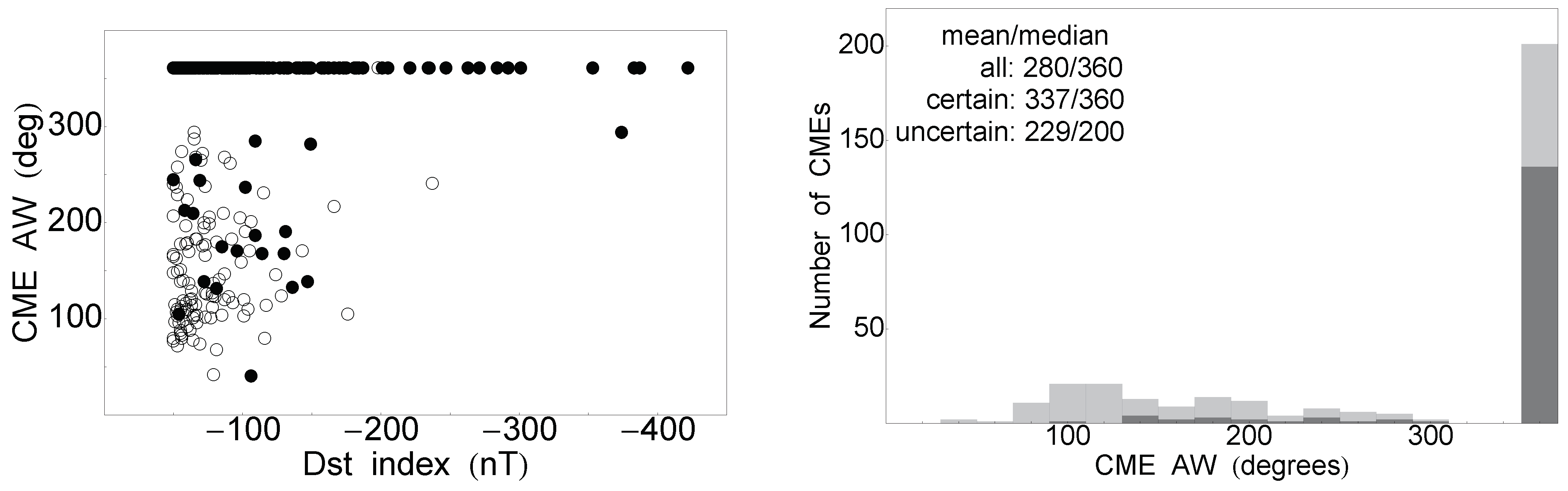
- Dst–CME speed: (330) vs. 0.30 (80);
- Dst–CME AW: (330) vs. 0.26 (80);
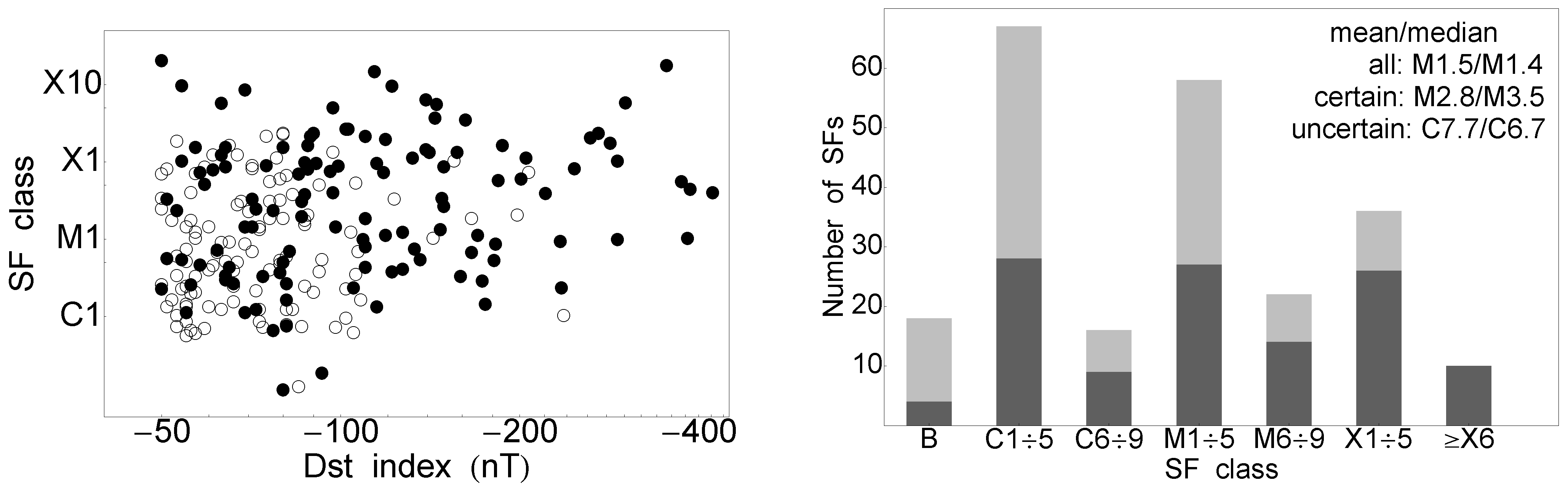
- Dst–SF class: (227) vs. 0.19 (61);
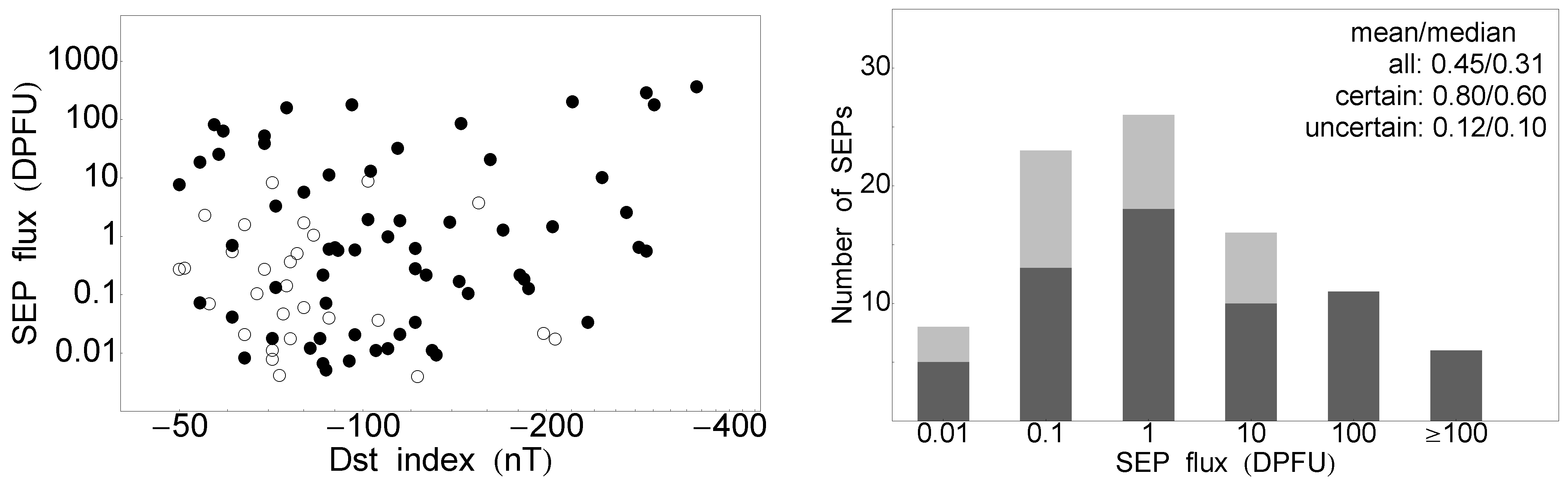
- Dst–SEP flux: (90) vs. 0.35 (38);
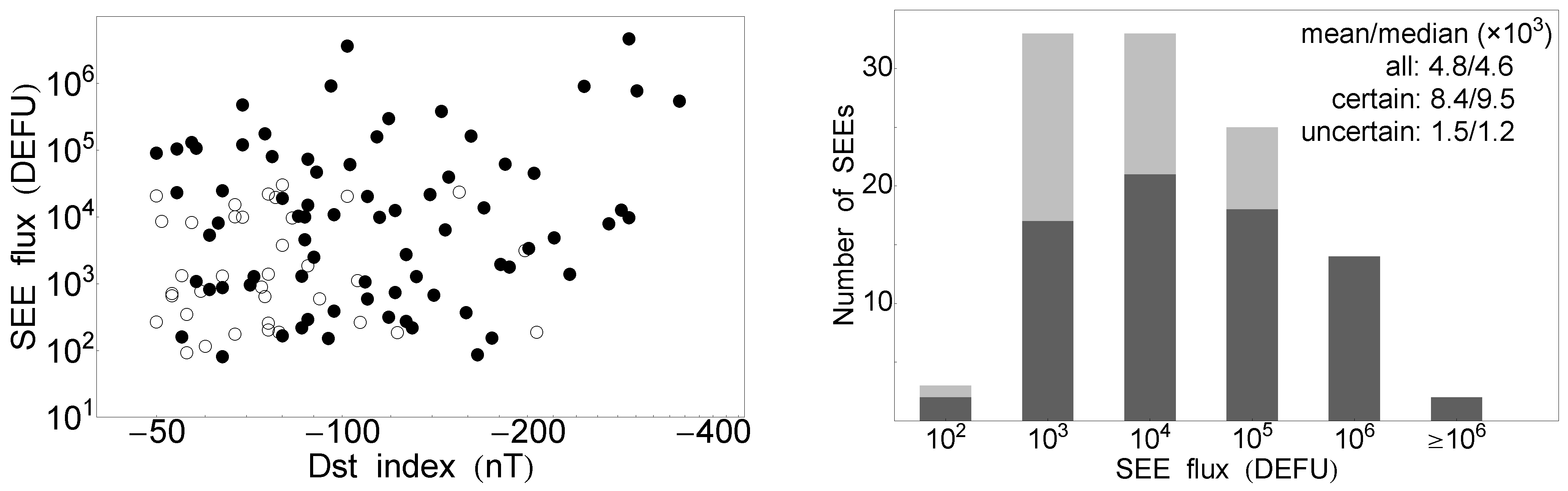
- Dst–SEE flux: (110) vs. 0.27 (33).
5. Conclusions
- Half of the GSs were linked to the arrival of an ICME with IP shocks also present;
- There were similar numbers of CMEs (halo and high speed, 330) and ICMEs (228);
- CME to ICME deceleration during its propagation in the solar wind was from 1000/874 to 483/460 kms in mean/median values;
- No correlation was found between the Dst and the parameters of the solar events (CME speed, CME AW, SF class, or SEP/SEE flux);
- The GS-related solar events originated close to the solar disk center.
Author Contributions
Funding
Institutional Review Board Statement
Informed Consent Statement
Data Availability Statement
Acknowledgments
Conflicts of Interest
Abbreviations
| ACE/EPAM | Satellite and instrument for particle detection |
| AU | Astronomical unit |
| AW | Angular width |
| CDAW | Coordinated Data Analyses Workshop |
| CIR | Co-rotating interaction region |
| CME | Coronal mass ejection |
| DEFU | Differential electron flux units |
| DPFU | Differential proton flux units |
| GIC | Geomagnetically induced current |
| GS | Geomagnetic storm |
| HSS | High-speed solar wind stream |
| ICME | Interplanetary CME |
| IMF | Interplanetary magnetic field |
| IP | Interplanetary |
| MPA | Measurement position angle |
| NASA | National Aeronautics and Space Administration |
| NOAA | National Oceanic and Atmospheric Administration |
| SC | Solar cycle |
| SEE | Solar energetic electron |
| SEP | Solar energetic proton |
| SF | Solar flare |
| SOHO/LASCO | Satellite and instrument for CME detection |
| SSC | Sudden storm commencement |
| SXR | Soft X-ray |
| Wind/EPACT | Satellite and instrument for particle detection |
Appendix A. Summary of Occurrence Rates

| Type | SC23 | SC24 | SC23+24 |
|---|---|---|---|
| ICMEs | 44% (159/361) | 37% (69/185) | 42% (228/546) |
| IP shocks | 35% (127/361) | 14% (52/185) | 33% (179/546) |
| CMEs | 61% (220/361) | 59% (110/185) | 60% (330/546) |
| - certain | 32% (114/361) | 23% (43/185) | 29% (157/546) |
| SFs | 43% (157/361) | 39% (70/185) | 42% (227/546) |
| - certain | 24% (86/361) | 17% (32/185) | 22% (118/546) |
| SEPs | 16% (57/361) | 19% (33/185) | 16% (90/546) |
| - certain | 12% (43/361) | 11% (20/185) | 12% (63/546) |
| SEEs | 19% (69/361) | 22% (41/185) | 20% (110/546) |
| - certain | 14% (51/361) | 12% (23/185) | 14% (74/546) |
Appendix B. Catalog of GSs with Proposed IP and Solar Origin (1996–2019)
| GS | ICME | IP Shock | CME | SF | SEP | SEE | ||||||
|---|---|---|---|---|---|---|---|---|---|---|---|---|
| yyyy | mm | dd | h | Dst | Speed | Speed | Speed | AW | Class | Location | Flux | Flux |
| 1996 | 1 | 13 | 11 | −90 | no | no | 499 u | 18 | no | no | no | no |
| 1996 | 3 | 11 | 4 | −60 | no | no | u | u | no | no | no | no |
| 1996 | 3 | 20 | 24 | −54 | no | no | 418 u | 59 | no | no | no | no |
| 1996 | 3 | 21 | 23 | −66 | no | no | u | u | no | no | no | no |
| 1996 | 3 | 24 | 3 | −53 | no | no | u | u | no | no | no | no |
| 1996 | 3 | 25 | 2 | −60 | no | no | u | u | no | no | no | no |
| 1996 | 4 | 15 | 1 | −56 | no | no | u | u | no | no | no | no |
| 1996 | 4 | 17 | 9 | −52 | no | no | u | u | no | no | no | no |
| 1996 | 9 | 12 | 9 | −54 | no | no | u | u | no | no | no | no |
| 1996 | 9 | 23 | 8 | −51 | no | no | 410 | 27 | no | no | no | no |
| 1996 | 9 | 27 | 1 | −50 | no | no | u | u | no | no | no | no |
| 1996 | 10 | 19 | 17 | −52 | no | no | u | u | no | no | no | no |
| 1996 | 10 | 23 | 5 | −105 | no | no | 470 u | 170 | B6.0 | no | no | no |
| 1997 | 1 | 10 | 10 | −78 | 450 | 434 | 136 | 360 | no | no | no | no |
| 1997 | 2 | 10 | 11 | −68 | 450 | 618 | 490 | 360 | no | no | no | no |
| 1997 | 2 | 11 | 10 | −60 | no | no | u | u | no | no | no | no |
| 1997 | 2 | 17 | 9 | −54 | no | no | u | u | no | no | no | no |
| 1997 | 2 | 27 | 24 | −86 | no | 543 | 905 u | 209 | B7.2 | no | no | no |
| 1997 | 3 | 28 | 24 | −63 | no | no | u | u | no | no | no | no |
| 1997 | 4 | 11 | 5 | −82 | 460 | 337 | 878 | 360 | C6.8 | S30E19 | 0.0118 | no |
| 1997 | 4 | 17 | 6 | −77 | no | 389 | dg | dg | no | no | no | no |
| 1997 | 4 | 22 | 1 | −107 | 360 | no | u | u | no | no | no | no |
| 1997 | 5 | 2 | 1 | −64 | no | 361 | 255 u | 360 | no | no | no | no |
| 1997 | 5 | 15 | 13 | −115 | 450 | 443 | 464 u | 360 | C1.3 | no | 0.0202 | no |
| 1997 | 5 | 27 | 5 | −73 | 340 | 303 | 296 u | 165 | M1.3 | N05W12 | 0.004 | no |
| 1997 | 6 | 9 | 4 | −84 | 380 | no | u | u | no | no | no | no |
| 1997 | 9 | 3 | 23 | −98 | 410 | 368 | 371 | 360 | M1.4 | N30E17 | no | no |
| 1997 | 9 | 18 | 6 | −56 | no | no | u | u | no | no | no | no |
| 1997 | 10 | 1 | 16 | −98 | 450 | no | 359 | 360 | no | no | no | no |
| 1997 | 10 | 10 | 20 | −65 | 430 | 471 | 506 | 103 | no | no | no | no |
| 1997 | 10 | 11 | 4 | −130 | 400 | no | 1271 | 167 | no | no | 0.0108 | 213 |
| 1997 | 10 | 25 | 3 | −64 | no | no | 523 | 360 | C3.3 | N16E07 | no | 79 |
| 1997 | 10 | 27 | 23 | −60 | 500 | no | 503 | 360 | no | no | no | no |
| 1997 | 11 | 7 | 5 | −110 | 400 | no | 785 | 360 | X2.1 | S14W33 | 0.9518 | 19,795 |
| 1997 | 11 | 10 | 3 | −54 | no | no | 1556 | 360 | X9.4 | S18W63 | 18.13 | 102,017 |
| 1997 | 11 | 23 | 7 | −108 | 510 | 377 | 611 u | 360 | C1.6 | no | no | no |
| 1997 | 12 | 11 | 11 | −60 | 350 | 375 | 397 u | 223 | no | no | no | no |
| 1997 | 12 | 30 | 20 | −77 | 370 | 386 | 197 u | 360 | no | no | no | no |
| 1998 | 1 | 7 | 5 | −77 | 400 | 406 | 438 | 360 | B6.4 | N24W42 | no | no |
| 1998 | 1 | 30 | 12 | −55 | 380 | no | 693 | 360 | C1.1 | N21E25 | no | no |
| 1998 | 2 | 18 | 1 | −100 | 400 | no | u | u | no | no | no | no |
| 1998 | 2 | 18 | 20 | −51 | 440 | 451 | u | u | no | no | no | no |
| 1998 | 2 | 20 | 1 | −50 | no | no | u | u | no | no | no | no |
| 1998 | 3 | 10 | 21 | −116 | no | no | 659 u | 79 | no | no | no | no |
| 1998 | 3 | 21 | 16 | −85 | no | no | 636 | 174 | no | no | no | no |
| 1998 | 3 | 25 | 17 | −56 | 400 | no | u | u | no | no | no | no |
| 1998 | 3 | 29 | 20 | −54 | no | no | 761 | 104 | C5.3 | no | no | no |
| 1998 | 4 | 24 | 8 | −69 | no | 402 | 1863 | 243 | M1.4 | u | 37.6 | 461,152 |
| 1998 | 4 | 26 | 18 | −63 | no | no | 1691 | 360 | X1.2 | S17E102 | no | no |
| 1998 | 5 | 2 | 18 | −85 | 520 | 631 | 1374 | 360 | M6.8 | S18E20 | 0.0173 | 9955 |
| 1998 | 5 | 4 | 6 | −205 | 550 | 474 | 938 | 360 | X1.1 | S15W15 | 1.423 | 43,760 |
| 1998 | 6 | 6 | 22 | −50 | no | no | 818 | 147 | no | no | no | no |
| 1998 | 6 | 14 | 11 | −55 | 340 | 273 | 1223 u | 177 | M1.4 | no | no | no |
| 1998 | 6 | 26 | 5 | −101 | 470 | no | 278 u | 119 | no | no | no | u |
| 1998 | 7 | 16 | 17 | −58 | no | no | dg | dg | no | no | no | no |
| 1998 | 8 | 6 | 12 | −138 | 360 | 475 | dg | dg | no | no | no | no |
| 1998 | 8 | 7 | 6 | −108 | 450 | no | dg | dg | no | no | no | no |
| 1998 | 8 | 20 | 21 | −67 | 320 | 321 | dg | dg | no | no | no | no |
| 1998 | 8 | 27 | 10 | −155 | 650 | 708 | dg | dg | X1.0 | no | 3.609 | 22,947 |
| 1998 | 9 | 1 | 17 | −55 | no | no | dg | dg | no | no | no | no |
| 1998 | 9 | 18 | 14 | −51 | no | no | dg | dg | no | no | no | no |
| 1998 | 9 | 25 | 10 | −207 | 640 | 768 | dg | dg | M7.1 | N18E09 | 0.0167 | 182 |
| 1998 | 10 | 1 | 2 | −58 | no | no | dg | dg | no | no | no | no |
| 1998 | 10 | 2 | 22 | −56 | no | 660 | dg | dg | no | no | no | no |
| 1998 | 10 | 7 | 23 | −70 | no | no | dg | dg | no | no | no | no |
| 1998 | 10 | 19 | 16 | −112 | 390 | no | 262 | 360 | no | no | no | no |
| 1998 | 10 | 20 u | 22 | −71 | no | no | u | u | no | no | no | no |
| 1998 | 10 | 22 u | 19 | −53 | 520 | no | u | u | no | no | no | no |
| 1998 | 11 | 6 | 9 | −61 | no | no | 661 u | 169 | C4.4 | S25E44 | no | no |
| 1998 | 11 | 7 u | 17 | −81 | 450 | no | 523 | 360 | C1.6 | N11W01 | no | no |
| 1998 | 11 | 8 | 7 | −149 | 450 | 645 | 1118 | 360 | M8.4 | N22W18 | no | u |
| 1998 | 11 | 9 | 18 | −142 | no | no | u | u | no | no | no | no |
| 1998 | 11 | 13 | 22 | −131 | 390 | 406 | 325 | 190 | no | no | no | no |
| 1998 | 12 | 11 | 16 | −69 | no | no | 806 u | 73 | no | no | no | no |
| 1998 | 12 | 25 | 12 | −57 | no | no | 752 u | 22 | no | no | no | no |
| 1998 | 12 | 29 | 12 | −58 | 400 | 464 | u | u | no | no | no | no |
| 1999 | 1 | 14 | 1 | −112 | 420 | 413 | u | u | no | no | no | no |
| 1999 | 1 | 23 | 23 | −52 | 570 | 701 | dg | dg | no | no | no | no |
| 1999 | 2 | 18 | 10 | −123 | 540 | 700 | dg | dg | M3.2 | S23W14 | 0.0038 | 180 |
| 1999 | 3 | 1 | 1 | −94 | no | no | u | u | no | no | no | no |
| 1999 | 3 | 4 | 24 | −52 | no | no | u | u | no | no | no | no |
| 1999 | 3 | 7 | 11 | −57 | no | no | u | u | no | no | no | no |
| 1999 | 3 | 10 | 9 | −81 | 410 | 501 | u | u | no | no | no | no |
| 1999 | 3 | 29 | 15 | −56 | no | no | u | u | no | no | no | no |
| 1999 | 4 | 17 | 8 | −91 | 410 | 456 | 291 u | 261 | no | no | no | no |
| 1999 | 7 | 31 | 2 | −53 | 480 | no | 462 | 360 | M2.3 | S15E03 | no | no |
| 1999 | 8 | 23 | 1 | −66 | 460 | no | 736 | 265 | C2.6 | N23E27 | no | no |
| 1999 | 9 | 13 | 5 | −74 | no | 531 | 1467 u | 125 | B7.0 | no | no | no |
| 1999 | 9 | 16 | 9 | −67 | no | 544 | 898 u | 182 | C4.9 | N21E02 | no | no |
| 1999 | 9 | 22 | 24 | −173 | 530 | 466 | 604 | 360 | C2.8 | no | no | no |
| 1999 | 9 | 27 | 19 | −64 | no | no | 1150 u | 77 | no | no | no | no |
| 1999 | 9 | 30 | 4 | −61 | no | no | u | u | no | no | no | no |
| 1999 | 10 | 10 | 19 | −67 | no | no | u | u | no | no | no | no |
| 1999 | 10 | 22 | 7 | −237 | 480 | 476 | 144 u | 240 | C1.0 | no | no | no |
| 1999 | 10 | 28 | 18 | −66 | no | no | 1127 u | 114 | C1.5 | u | no | no |
| 1999 | 11 | 7 | 16 | −67 | no | no | u | u | no | no | no | no |
| 1999 | 11 | 8 | 15 | −73 | no | no | u | u | no | no | no | no |
| 1999 | 11 | 11 | 7 | −55 | no | no | 631 u | 87 | C5.0 | u | no | no |
| 1999 | 11 | 13 | 9 | −69 | 450 | no | dg | dg | no | no | no | no |
| 1999 | 11 | 13 | 23 | −106 | 440 | 466 | dg | dg | no | no | no | no |
| 1999 | 11 | 16 | 17 | −79 | no | no | 1104 u | 41 | C4.6 | S12E44 | no | no |
| 1999 | 11 | 24 | 10 | −50 | no | no | dg | dg | no | no | no | no |
| 1999 | 12 | 13 | 10 | −85 | 440 | 553 | dg | dg | no | no | no | no |
| 1999 | 12 | 31 | 24 | −50 | no | no | u | u | no | no | no | no |
| 2000 | 1 | 11 | 22 | −81 | no | no | 1813 u | 67 | C5.8 | N23W42 | no | no |
| 2000 | 1 | 23 | 1 | −97 | 380 | no | 739 | 360 | M3.9 | S19E11 | 0.0201 | 381 |
| 2000 | 2 | 12 | 12 | −133 | 540 | 638 | 1003 | 360 | C7.3 | N31E04 | no | no |
| 2000 | 3 | 31 | 12 | −60 | 420 | no | 1177 | 360 | u | u | u | u |
| 2000 | 4 | 5 | 2 | −63 | no | no | 532 u | 113 | no | no | no | no |
| 2000 | 4 | 7 | 1 | −292 | 560 | 642 | 1188 | 360 | C9.7 | N16W66 | 0.5441 | 9431 |
| 2000 | 4 | 16 | 12 | −79 | no | no | 409 u | 360 | M3.1 | S14W01 | no | no |
| 2000 | 4 | 24 | 15 | −61 | 500 | no | u | u | no | no | no | no |
| 2000 | 5 | 17 | 6 | −92 | 550 | no | 666 u | 182 | C3.7 | S22E65 | no | no |
| 2000 | 5 | 24 | 9 | −147 | 530 | 656 | 629 | 138 | no | no | no | no |
| 2000 | 5 | 29 | 21 | −54 | no | no | u | u | no | no | no | no |
| 2000 | 6 | 8 | 20 | −90 | 610 | no | 1119 | 360 | X2.3 | N20E18 | 0.6162 | 2432 |
| 2000 | 6 | 26 | 18 | −76 | 520 | no | 847 u | 198 | M3.0 | N26W72 | 0.017 | 21,306 |
| 2000 | 7 | 16 | 1 | −301 | 740 | no | 1674 | 360 | X5.7 | N22W07 | 174.3 | 750,613 |
| 2000 | 7 | 20 | 10 | −93 | 530 | 638 | 788 u | 116 | C5.3 | N13E30 | no | no |
| 2000 | 7 | 22 | 18 | −63 | no | 497 | dg | dg | no | no | no | no |
| 2000 | 7 | 23 | 23 | −68 | 360 | no | dg | dg | no | no | no | no |
| 2000 | 7 | 29 | 12 | −71 | 440 | no | 1287 u | 271 | M8.0 | N06W08 | no | no |
| 2000 | 8 | 11 | 7 | −106 | 430 | 380 | 597 | 40 | no | no | no | no |
| 2000 | 8 | 12 | 10 | −235 | 580 | 563 | 702 | 360 | C2.3 | N11W11 | no | no |
| 2000 | 8 | 29 | 7 | −60 | no | no | 518 u | 178 | M1.4 | S15E67 | no | no |
| 2000 | 9 | 12 | 20 | −73 | no | no | 761 u | 176 | no | no | u | u |
| 2000 | 9 | 17 | 24 | −201 | 600 | no | 1215 | 360 | M5.9 | N14E07 | no | 3300 |
| 2000 | 9 | 19 | 15 | −77 | no | no | 1056 u | 100 | no | no | no | no |
| 2000 | 9 | 26 | 3 | −55 | no | no | u | u | no | no | no | no |
| 2000 | 9 | 30 | 15 | −76 | no | 454 | 587 u | 360 | M1.8 | N09W18 | no | 250 |
| 2000 | 10 | 3 | 13 | −79 | no | 462 | 820 u | 136 | C5.2 | N17W52 | no | 181 |
| 2000 | 10 | 4 | 21 | −143 | 400 | no | 703 u | 170 | M1.0 | S22E36 | no | no |
| 2000 | 10 | 5 | 8 | −175 | no | 538 | 525 | 360 | C1.4 | S09E07 | no | 149 |
| 2000 | 10 | 5 | 14 | −182 | 450 | no | 569 | 360 | C8.4 | no | no | u |
| 2000 | 10 | 13 | 6 | −71 | no | 526 | 798 u | 175 | C6.7 | N01W14 | 0.0075 | no |
| 2000 | 10 | 14 | 15 | −107 | 400 | no | 506 u | 360 | u | u | no | 257 |
| 2000 | 10 | 23 | 8 | −53 | no | no | u | u | no | no | no | no |
| 2000 | 10 | 29 | 4 | −127 | 380 | 390 | 770 | 360 | C4.0 | N06W60 | 0.2115 | 2665 |
| 2000 | 11 | 4 | 10 | −50 | no | 429 | 801 | 360 | C2.2 | S17E39 | no | no |
| 2000 | 11 | 6 | 22 | −159 | 510 | 611 | 291 | 360 | C3.2 | N02W02 | no | 357 |
| 2000 | 11 | 10 | 13 | −96 | no | 925 | 1738 | 170 | M7.4 | N10W77 | 173.2 | 888,533 |
| 2000 | 11 | 27 | 2 | −80 | 540 | 524 | 1245 u | 360 | X2.3 | N22W07 | 1.643 | 29,353 |
| 2000 | 11 | 29 | 14 | −119 | 540 | 604 | 671 | 360 | X1.9 | N20W23 | no | 28,8203 |
| 2000 | 12 | 23 | 5 | −62 | 320 | 314 | 510 | 360 | C7.0 | N15S01 | no | no |
| 2001 | 1 | 24 | 19 | −61 | 400 | 615 | 1507 | 360 | M7.7 | S07S46 | 0.0399 | 793 |
| 2001 | 2 | 13 | 22 | −50 | no | 651 | 956 u | 360 | no? | N37W03 | no | no |
| 2001 | 3 | 5 | 3 | −73 | 440 | no | 631 u | 237 | C1.2 | S09W27 | no | no |
| 2001 | 3 | 20 | 14 | −149 | 360 | 441 | 271 | 281 | no | no | no | no |
| 2001 | 3 | 23 | 17 | −75 | no | 382 | 389 u | 360 | no | N20W0 | no | no |
| 2001 | 3 | 28 | 16 | −87 | 610 | 552 | 906 u | 360 | M1.7 | N15E22 | no | u |
| 2001 | 3 | 31 | 9 | −387 | 640 | 498 | 519 | 360 | M4.3 | S10E30 | no | no |
| 2001 | 3 | 31 | 22 | −284 | 600 | 565 | 942 | 360 | X1.7 | N20E19 | 0.6266 | 12,355 |
| 2001 | 4 | 5 | 8 | −50 | 650 | 845 | 2505 | 244 | X20 | no | 7.389 | 87782 |
| 2001 | 4 | 9 | 7 | −63 | 740 | 696 | 1270 | 360 | X5.6 | S21E31 | no | u |
| 2001 | 4 | 11 | 24 | −271 | 640 | 310 | 2411 | 360 | X2.3 | S23W09 | 2.499 | 7716 |
| 2001 | 4 | 13 | 16 | −77 | 730 | no | 1103 | 360 | M2.3 | S22W27 | no | 77,982 |
| 2001 | 4 | 18 | 7 | −114 | 430 | 602 | 1199 | 167 | X14.4 | S20W85 | 31.3 | 153,434 |
| 2001 | 4 | 22 | 16 | −102 | 350 | 381 | 2465 u | 360 | C2.2 | S15W90 | 8.5 | 19,759 |
| 2001 | 5 | 10 | 4 | −76 | 430 | no | 1223 u | 205 | C3.9 | N25W35 | 0.3542 | 1356 |
| 2001 | 6 | 18 | 9 | −61 | no | 336 | 1701 | 360 | no | no | 0.6736 | 5220 |
| 2001 | 8 | 17 | 22 | −105 | 500 | 519 | 618 | 360 | C2.3 | N24W19 | 0.0107 | no |
| 2001 | 9 | 13 | 8 | −57 | 410 | 449 | 791 u | 360 | C3.2 | N13E35 | no | u |
| 2001 | 9 | 23 | 19 | −73 | 440 | no | 436 u | 360 | no | no | no | no |
| 2001 | 9 | 26 | 2 | −102 | no | 851 | 2402 | 360 | X2.6 | S16E23 | 1.88 | 3,551,563 |
| 2001 | 9 | 30 | 21 | −66 | 560 | 483 | 509 u | 182 | C3.8 | S20W27 | no | no |
| 2001 | 10 | 1 | 9 | −148 | 490 | no | 846 | 360 | M3.3 | S18W36 | no | no |
| 2001 | 10 | 2 | 13 | −104 | 490 | no | 773 u | 109 | M1.2 | no | no | no |
| 2001 | 10 | 3 | 15 | −166 | 500 | no | 509 u | 216 | M1.8 | N13E03 | no | no |
| 2001 | 10 | 9 | 16 | −64 | no | 382 | 1537 | 360 | no | no | no | no |
| 2001 | 10 | 12 | 13 | −71 | 560 | 579 | 973 | 360 | M1.4 | S28E08 | no | no |
| 2001 | 10 | 19 | 22 | −57 | no | no | u | u | no | no | no | no |
| 2001 | 10 | 21 | 22 | −187 | 460 | 636 | 901 | 360 | X1.6 | N15W29 | 0.1236 | 1739 |
| 2001 | 10 | 28 | 12 | −157 | 360 | 589 | 1092 | 360 | X1.3 | S16W21 | no | no |
| 2001 | 11 | 1 | 11 | −106 | 330 | 395 | 592 u | 200 | C3.4 | no | no | no |
| 2001 | 11 | 6 | 7 | −292 | 600 | no | 1810 | 360 | X1.0 | N06W18 | 277.3 | 4,512,846 |
| 2001 | 11 | 24 | 17 | −221 | 720 | 804 | 1443 | 360 | M3.8 | S25W67 | 196.7 | 4715 |
| 2001 | 12 | 21 | 23 | −67 | no | 552 | 1025 u | 103 | no | no | no | 170 |
| 2001 | 12 | 24 | 11 | −55 | no | 306 | 769 u | 108 | C2.4 | no | no | no |
| 2001 | 12 | 30 | 6 | −58 | 400 | 669 | 1446 | 212 | M7.1 | N08W54 | 24.47 | 103,570 |
| 2002 | 1 | 11 | 7 | −72 | no | no | 1794 | 360 | no | no | no | no |
| 2002 | 2 | 2 | 10 | −86 | no | no | 1136 | 360 | no | no | 0.2095 | 1267 |
| 2002 | 2 | 5 | 21 | −82 | no | no | u | u | no | no | no | no |
| 2002 | 3 | 1 | 2 | −71 | 390 | no | u | u | no | no | no | no |
| 2002 | 3 | 24 | 10 | −100 | 450 | 517 | 603 | 360 | no | no | no | no |
| 2002 | 4 | 18 | 8 | −127 | 480 | 517 | 720 | 360 | M1.2 | S15W01 | no | 267 |
| 2002 | 4 | 19 u | 19 | −126 | no | 768 | u | u | no | no | no | no |
| 2002 | 4 | 20 | 9 | −149 | 500 | no | 1240 | 360 | M2.6 | S14W34 | 0.1024 | 38,361 |
| 2002 | 4 | 23 | 16 | −57 | no | 644 | 2393 | 360 | X1.5 | S14W84 | 79.07 | 127,221 |
| 2002 | 5 | 11 | 20 | −110 | 430 | 483 | 614 | 360 | C4.2 | S12W07 | no | no |
| 2002 | 5 | 14 | 21 | −63 | no | no | 1154 u | 120 | C1.2 | S18W43 | no | no |
| 2002 | 5 | 19 | 7 | −58 | no | 545 | 600 | 360 | C4.5 | S23E15 | no | no |
| 2002 | 5 | 23 | 18 | −109 | 590 | 737 | 1246 | 186 | C9.7 | N17E36 | no | 1032 |
| 2002 | 5 | 27 | 9 | −64 | no | no | 1557 u | 360 | C5.0 | S30W34 | 1.517 | no |
| 2002 | 8 | 1 | 14 | −51 | no | no | u | u | no | no | no | no |
| 2002 | 8 | 2 | 6 | −102 | 460 | 496 | 562 | 236 | no | no | no | no |
| 2002 | 8 | 02 u | 23 | −69 | no | no | u | u | no | no | no | no |
| 2002 | 8 | 4 | 6 | −58 | no | no | u | u | no | no | no | no |
| 2002 | 8 | 19 | 8 | −53 | no | 672 | u | u | no | no | no | no |
| 2002 | 8 | 20 | 1 | −71 | no | 535 | u | u | no | no | no | no |
| 2002 | 8 | 21 | 7 | −106 | 460 | no | 1585 u | 360 | M5.2 | S14E20 | 0.0349 | 1082 |
| 2002 | 9 | 4 | 6 | −109 | no | 340 | u | u | no | no | no | no |
| 2002 | 9 | 8 | 1 | −181 | 470 | 897 | 1748 | 360 | C5.2 | N09E28 | 0.2118 | 1886 |
| 2002 | 9 | 10 | 1 | −69 | no | no | 909 u | 360 | no | no | no | no |
| 2002 | 9 | 11 | 23 | −90 | no | no | u | u | no | no | no | no |
| 2002 | 10 | 1 | 21 | −176 | 390 | 331 | 881 u | 104 | no | no | no | no |
| 2002 | 10 | 2 u | 5 | −158 | no | no | u | u | no | no | no | no |
| 2002 | 10 | 4 | 9 | −146 | 430 | no | u | u | no | no | no | no |
| 2002 | 10 | 5 | 16 | −102 | no | no | 903 u | 190 | B9.2 | S18E20 | no | no |
| 2002 | 10 | 7 | 8 | −115 | no | no | 743 u | 230 | no | no | no | no |
| 2002 | 10 | 8 u | 5 | −108 | no | no | u | u | no | no | no | no |
| 2002 | 10 | 14 | 14 | −100 | no | no | u | u | no | no | no | no |
| 2002 | 10 | 15 u | 19 | −70 | no | no | 1009 u | 264 | M2.2 | S08E66 | no | u |
| 2002 | 10 | 16 | 21 | −63 | no | no | 1694 u | 360 | no | no | no | no |
| 2002 | 10 | 24 | 21 | −98 | no | no | 640 u | 360 | no | no | no | no |
| 2002 | 10 | 25 u | 2 | −91 | no | no | u | u | no | no | no | no |
| 2002 | 10 | 26 u | 20 | −62 | no | no | 1052 u | 119 | C6.6 | S04W62 | no | no |
| 2002 | 10 | 27 u | 16 | −65 | no | no | 689 u | 286 | no | no | no | no |
| 2002 | 10 | 28 u | 5 | −63 | no | no | 629 u | 360 | no | no | no | no |
| 2002 | 10 | 30 u | 19 | −52 | no | no | 2115 u | 360 | no | no | no | no |
| 2002 | 11 | 3 | 4 | −74 | no | no | u | u | no | no | no | no |
| 2002 | 11 | 18 | 23 | −52 | 380 | no | 1185 | 360 | no | no | no | no |
| 2002 | 11 | 20 | 21 | −87 | no | 392 | 1008 u | 119 | C2.4 | no | no | no |
| 2002 | 11 | 21 | 11 | −128 | no | no | 938 u | 123 | no | no | no | no |
| 2002 | 11 | 27 | 7 | −64 | no | no | 1077 | 360 | no | no | no | 851 |
| 2002 | 12 | 19 | 21 | −72 | no | no | u | u | no | no | no | no |
| 2002 | 12 | 20 u | 6 | −64 | no | no | u | u | no | no | no | no |
| 2002 | 12 | 21 u | 4 | −75 | 440 | no | u | u | no | no | no | no |
| 2002 | 12 | 23 | 12 | −67 | no | no | 1092 u | 360 | M2.7 | N15W09 | 0.1002 | 9777 |
| 2002 | 12 | 27 | 5 17 | −68 | no | no | u | u | no | no | no | no |
| 2003 | 1 | 30 | 1 | −66 | no | no | 1053 u | 267 | C2.4 | S17W23 | no | no |
| 2003 | 2 | 2 | 18 | −72 | 510 | no | 620 | 138 | no | no | no | no |
| 2003 | 2 | 4 | 10 | −74 | no | no | u | u | no | no | no | no |
| 2003 | 2 | 4 u | 24 | −54 | no | no | u | u | no | no | no | no |
| 2003 | 2 | 27 | 22 | −66 | no | no | u | u | no | no | no | no |
| 2003 | 3 | 4 | 1 | −67 | no | no | u | u | no | no | no | no |
| 2003 | 3 | 16 | 22 | −60 | no | no | 1021 u | 91 | C1.3 | S12E09 | dg | no |
| 2003 | 3 | 20 | 20 | −64 | 650 | no | 1601 | 209 | X1.5 | S15W46 | 0.008 | 23,895 |
| 2003 | 3 | 27 | 18 | −56 | no | no | 1505 u | 82 | C1.9 | S17E77 | no | no |
| 2003 | 3 | 29 u | 7 | −63 | no | no | u | u | no | no | no | no |
| 2003 | 3 | 29 u | 21 | −70 | no | no | u | u | no | no | no | no |
| 2003 | 3 | 31 u | 16 | −78 | no | no | 664 u | 111 | no | no | no | no |
| 2003 | 4 | 2 | 23 | −53 | no | no | u | u | no | no | no | no |
| 2003 | 4 | 4 | 24 | −62 | no | no | 885 u | 87 | no | no | no | no |
| 2003 | 4 | 25 | 23 | −53 | no | no | 899 u | 148 | B7.2 | no | no | no |
| 2003 | 4 | 30 | 3 | −67 | no | no | 991 u | 95 | no | no | no | no |
| 2003 | 5 | 10 | 9 | −84 | 680 | no | u | u | no | no | no | no |
| 2003 | 5 | 22 | 3 | −73 | no | no | 866 u | 101 | B8.3 | u | no | no |
| 2003 | 5 | 30 | 1 | −144 | 600 | 907 | 1366 | 360 | X3.6 | S07W20 | 0.1636 | no |
| 2003 | 5 | 31 | 6 | −63 | 680 | no | 1237 | 360 | X1.2 | S06W37 | no | 7886 |
| 2003 | 6 | 2 | 9 | −91 | no | no | 1835 | 360 | M9.3 | S07W65 | 0.5543 | 45,772 |
| 2003 | 6 | 8 | 23 | −50 | no | no | 1458 u | 239 | no | no | no | no |
| 2003 | 6 | 16 u | 17 | −59 | no | no | u | u | no | no | no | no |
| 2003 | 6 | 16 | 23 | −68 | 510 | no | u | u | no | no | no | no |
| 2003 | 6 | 17 | 9 | −81 | no | no | 1215 u | 179 | no | no | no | no |
| 2003 | 6 | 18 | 10 | −141 | 480 | 479 | 2053 | 360 | X1.3 | S07E80 | no | 656 |
| 2003 | 6 | 21 | 10 | −50 | no | no | 1813 u | 360 | M6.8 | S08E58 | 0.2634 | 20,103 |
| 2003 | 6 | 24 | 14 | −55 | no | no | u | u | no | no | no | no |
| 2003 | 7 | 11 | 11 | −55 | no | no | u | u | no | no | no | no |
| 2003 | 7 | 12 | 6 | −105 | no | no | u | u | no | no | no | no |
| 2003 | 7 | 16 | 14 | −90 | no | no | u | u | no | no | no | no |
| 2003 | 7 | 19 | 1 | −50 | no | no | u | u | no | no | no | no |
| 2003 | 7 | 27 | 8 | −57 | no | no | u | u | no | no | no | no |
| 2003 | 8 | 6 | 7 | −60 | 440 | no | 699 u | 360 | no | no | no | no |
| 2003 | 8 | 7 | 22 | −61 | no | no | u | u | no | no | no | no |
| 2003 | 8 | 18 | 16 | −148 | 450 | no | 378 | 360 | no | no | no | no |
| 2003 | 8 | 21 | 24 | −68 | no | no | u | u | no | no | no | no |
| 2003 | 9 | 17 | 24 | −65 | no | no | u | u | no | no | no | no |
| 2003 | 9 | 24 | 8 | −59 | no | no | 646 | 360 | no | no | no | no |
| 2003 | 10 | 14 | 23 | −85 | no | no | u | u | no | no | no | no |
| 2003 | 10 | 17 | 7 | −53 | no | no | u | u | no | no | no | no |
| 2003 | 10 | 20 u | 22 | −57 | no | no | 627 u | 360 | no | no | no | no |
| 2003 | 10 | 22 u | 7 | −61 | 520 | no | u | u | no | no | no | no |
| 2003 | 10 | 27 | 5 | −52 | 470 | no | 1406 u | 236 | M1.7 | S04E13 | u | u |
| 2003 | 10 | 30 | 1 | −353 | 1300 | no | 2459 | 360 | X17.2 | S16E68 | 353.2 | 530,064 |
| 2003 | 10 | 30 | 23 | −383 | 800 | no | 2029 | 360 | M1.0 | S15W02 | no | no |
| 2003 | 11 | 4 | 11 | −69 | no | 759 | 2598 | 360 | X8.3 | S14W56 | 50.99 | 116,852 |
| 2003 | 11 | 11 | 14 | −62 | no | no | 2008 u | 360 | no | no | no | no |
| 2003 | 11 | 20 | 21 | −422 | 580 | 666 | 1660 | 360 | M3.9 | N00E18 | u | u |
| 2003 | 11 | 22 | 23 | −87 | no | no | 669 | 360 | M9.6 | N01W08 | 0.0694 | 9787 |
| 2003 | 12 | 6 | 5 | −55 | no | no | 1393 u | 150 | C7.2 | S19W91 | 2.225 | 1281 |
| 2003 | 12 | 8 u | 22 | −54 | no | no | 676 u | 95 | C2.2 | S17W38 | no | no |
| 2003 | 12 | 10 u | 20 | −51 | no | no | u | u | no | no | no | no |
| 2004 | 1 | 7 | 14 | −50 | no | no | 1469 u | 166 | C2.5 | no | no | no |
| 2004 | 1 | 15 | 17 | −50 | no | no | u | u | no | no | no | no |
| 2004 | 1 | 22 | 14 | −130 | 560 | no | 965 | 360 | no | no | no | no |
| 2004 | 1 | 25 u | 4 | −81 | 490 | no | 762 u | 360 | C1.2 | S19E29 | no | no |
| 2004 | 1 | 27 u | 2 | −62 | no | no | u | u | no | no | no | no |
| 2004 | 2 | 11 | 18 | −93 | no | no | u | u | no | no | no | no |
| 2004 | 3 | 9 | 24 | −72 | no | no | u | u | no | no | no | no |
| 2004 | 3 | 11 | 24 | −63 | no | no | u | u | no | no | no | no |
| 2004 | 4 | 4 | 1 | −117 | 440 | no | 652 u | 113 | no | no | no | no |
| 2004 | 4 | 5 | 20 | −62 | no | no | u | u | no | no | no | no |
| 2004 | 7 | 17 | 3 | −76 | no | no | 747 u | 360 | M5.4 | N12W52 | no | 198 |
| 2004 | 7 | 23 | 3 | −99 | 560 | 454 | 710 | 360 | M8.6 | N10E35 | no | no |
| 2004 | 7 | 25 | 17 | −136 | 560 | 561 | 899 | 132 | C5.3 | N04E10 | no | u |
| 2004 | 7 | 27 | 14 | −170 | 870 | 1086 | 1333 | 360 | M1.1 | N08E33 | 1.245 | 13,269 |
| 2004 | 8 | 9 | 22 | −51 | no | no | 1004 | 360 | no | no | no | no |
| 2004 | 8 | 30 | 23 | −129 | 390 | 483 | u | u | no | no | no | no |
| 2004 | 11 | 8 | 7 | −374 | 630 | 742 | 1055 | 293 | M5.4 | N08E18 | no | no |
| 2004 | 11 | 10 | 11 | −263 | 640 | 813 | 1759 | 360 | X2.0 | N09W17 | u | no |
| 2004 | 11 | 25 | 8 | −53 | no | no | 649 u | 102 | no | no | no | no |
| 2004 | 11 | 28 | 7 | −50 | no | no | u | u | no | no | no | no |
| 2004 | 12 | 13 | 3 | −56 | 400 | no | 611 | 360 | C2.5 | N01W07 | no | no |
| 2005 | 1 | 8 | 3 | −93 | 460 | 560 | 735 | 360 | B1.8 | S15E15 | no | no |
| 2005 | 1 | 12 | 11 | −50 | no | no | 870 u | 164 | M2.4 | S09E69 | no | no |
| 2005 | 1 | 17 | 4 | −65 | 520 | 539 | 455 | 360 | C4.2 | S06E15 | no | no |
| 2005 | 1 | 18 | 9 | −103 | no | no | 2861 | 360 | X2.6 | N14W08 | 12.71 | 59,664 |
| 2005 | 1 | 19 u | 11 | −80 | 800 | no | 2094 u | 360 | X2.2 | N13W19 | u | u |
| 2005 | 1 | 22 | 6 | −97 | no | no | 2020 u | 360 | X1.3 | N15W51 | no | no |
| 2005 | 2 | 7 | 22 | −57 | no | no | 711 u | 139 | no | no | no | no |
| 2005 | 2 | 18 | 3 | −80 | 410 | no | 1135 | 360 | C4.9 | S03W23 | no | 162 |
| 2005 | 3 | 7 | 1 | −54 | no | no | u | u | no | no | no | no |
| 2005 | 4 | 5 | 5 | −70 | no | 472 | u | u | no | no | no | no |
| 2005 | 4 | 12 | 6 | −62 | no | no | u | u | no | no | no | no |
| 2005 | 5 | 8 | 3 | −82 | no | 438 | u | u | no | no | no | no |
| 2005 | 5 | 8 | 19 | −110 | no | 476 | 1180 | 360 | C7.8 | N04W67 | no | no |
| 2005 | 5 | 15 | 9 | −247 | 630 | 858 | 1689 | 360 | M8.0 | N12E11 | 9.876 | 879,497 |
| 2005 | 5 | 20 | 9 | −83 | 430 | no | 405 u | 140 | C1.2 | N15W27 | no | u |
| 2005 | 5 | 30 | 14 | −113 | 460 | u | 586 | 360 | no | no | no | no |
| 2005 | 6 | 13 | 1 | −106 | 480 | no | u | u | no | no | no | no |
| 2005 | 6 | 23 | 11 | −85 | no | no | 614 u | 103 | B1.2 | S13W51 | no | no |
| 2005 | 7 | 9 | 21 | −55 | no | no | 772 u | 360 | C1.3 | S08E34 | no | no |
| 2005 | 7 | 10 | 21 | −92 | 430 | 533 | 683 u | 360 | M4.9 | N09E03 | no | 579 |
| 2005 | 7 | 18 | 7 | −67 | 420 | 378 | 2115 u | 360 | X1.2 | N11W90 | no | 14,743 |
| 2005 | 8 | 24 | 12 | −184 | 660 | 536 | 2378 | 360 | M5.6 | S13W65 | 0.1792 | 59,728 |
| 2005 | 8 | 31 | 20 | −122 | no | no | 1600 | 360 | no | no | 0.0328 | 714 |
| 2005 | 9 | 4 | 10 | −71 | pd | no | 1384 u | 360 | no | no | no | no |
| 2005 | 9 | 10 u | 23 | −73 | no | 544 | 1291 u | 126 | M1.4 | S12E88 | no | no |
| 2005 | 9 | 11 | 11 | −139 | 900 | 1147 | 2257 | 360 | X6.2 | S10E58 | no | no |
| 2005 | 9 | 12 u | 22 | −89 | 750 | 1048 | 1893 | 360 | X2.1 | S13E47 | no | no |
| 2005 | 9 | 13 u | 13 | −86 | 630 | no | 1922 | 360 | M3.0 | S16E39 | no | no |
| 2005 | 9 | 15 | 17 | −80 | 680 | 661 | 1866 | 360 | X1.5 | S09E10 | 5.515 | 18,409 |
| 2005 | 10 | 8 | 8 | −50 | no | no | u | u | no | no | no | no |
| 2005 | 10 | 31 | 21 | −74 | 360 | no | u | u | no | no | no | no |
| 2005 | 12 | 11 | 19 | −55 | 480 | no | 673 u | 360 | B5.5 | N15E14 | no | no |
| 2006 | 1 | 26 | 4 | −51 | no | no | u | u | no | no | no | no |
| 2006 | 3 | 7 | 2 | −52 | no | no | u | u | no | no | no | no |
| 2006 | 4 | 5 | 16 | −79 | no | no | u | u | no | no | no | no |
| 2006 | 4 | 9 | 8 | −82 | no | no | u | u | no | no | no | no |
| 2006 | 4 | 14 | 10 | −98 | 520 | no | u | u | no | no | no | no |
| 2006 | 5 | 6 | 22 | −53 | no | no | 487 u | 360 | C1.0 | S17W02 | no | no |
| 2006 | 8 | 20 | 2 | −79 | 400 | 460 | 888 | 360 | C3.6 | S14W13 | no | no |
| 2006 | 9 | 24 | 10 | −55 | no | 402 | u | u | no | no | no | no |
| 2006 | 10 | 1 | 6 | −51 | no | 356 | u | u | no | no | no | no |
| 2006 | 10 | 13 | 23 | −55 | no | no | u | u | no | no | no | no |
| 2006 | 10 | 29 | 9 | −50 | no | no | u | u | no | no | no | no |
| 2006 | 11 | 10 | 2 | −63 | no | 360 | 1994 u | 360 | C8.8 | no | no | no |
| 2006 | 11 | 30 | 14 | −74 | 420 | no | u | u | no | no | no | no |
| 2006 | 12 | 6 | 13 | −55 | no | no | u | u | no | no | no | no |
| 2006 | 12 | 15 | 8 | −162 | 740 | 1012 | 1774 | 360 | X3.4 | S06W23 | 20.17 | 158,754 |
| 2007 | 3 | 24 | 9 | −72 | no | no | u | u | no | no | no | no |
| 2007 | 4 | 1 | 9 | −63 | no | no | u | u | no | no | no | no |
| 2007 | 5 | 23 | 14 | −58 | no | no | 958 u | 106 | no | no | no | u |
| 2007 | 10 | 25 | 22 | −53 | no | 433 | u | u | no | no | no | no |
| 2007 | 11 | 20 | 21 | −59 | 460 | 442 | u | u | no | no | no | no |
| 2008 | 2 | 28 | 8 | −52 | no | no | u | u | no | no | no | no |
| 2008 | 3 | 9 | 6 | −86 | no | no | u | u | no | no | no | no |
| 2008 | 3 | 27 | 22 | −56 | no | no | 1103 u | 112 | M1.7 | S13E78 | no | no |
| 2008 | 9 | 4 | 5 | −51 | no | no | u | u | no | no | no | no |
| 2008 | 10 | 11 | 12 | −54 | no | no | u | u | no | no | no | no |
| 2009 | 7 | 22 | 7 | −83 | 330 | 337 | u | u | no | no | no | no |
| 2010 | 2 | 15 | 24 | −59 | no | 336 | 509 u | 360 | M8.3 | N26E11 | no | 744 |
| 2010 | 4 | 6 | 15 | −81 | 640 | no | 668 | 360 | B7.4 | S25W00 | no | no |
| 2010 | 4 | 12 | 2 | −67 | 410 | 465 | u | u | no | no | no | no |
| 2010 | 5 | 2 | 19 | −71 | no | no | u | u | no | no | no | no |
| 2010 | 5 | 29 | 13 | −80 | 360 | no | 427 | 360 | B1.1 | N13W31 | no | no |
| 2010 | 6 | 4 | 2 | −53 | no | no | u | u | no | no | no | no |
| 2010 | 8 | 4 | 2 20 | −74 | 530 | 537 | 850 | 360 | C3.2 | N20E36 | no | no |
| 2010 | 10 | 11 | 20 | −75 | no | no | u | u | no | no | no | no |
| 2011 | 2 | 4 | 22 | −63 | 430 | no | 437 | 360 | no | no | no | no |
| 2011 | 3 | 1 | 15 | −88 | no | no | u | u | no | no | no | no |
| 2011 | 3 | 11 | 6 | −83 | no | no | 2125 u | 360 | M3.7 | N31W53 | 1.012 | 9316 |
| 2011 | 4 | 6 | 19 | −60 | no | no | 2081 u | 109 | no | no | no | no |
| 2011 | 5 | 28 | 12 | −80 | 510 | no | 657 u | 122 | no | no | no | no |
| 2011 | 7 | 5 | 1 | −59 | nd | no | 511 u | 196 | no | no | no | no |
| 2011 | 8 | 6 | 4 | −115 | no | 577 | 1315 | 360 | M9.3 | N19W36 | 1.79 | 9625 |
| 2011 | 9 | 10 | 5 | −75 | 470 | no | 575 u | 360 | X2.1 | N14W18 | 0.1368 | 622 |
| 2011 | 9 | 17 | 16 | −72 | 430 | 506 | 746 u | 199 | no | no | no | no |
| 2011 | 9 | 26 | 24 | −118 | 580 | 556 | 1915 | 360 | M7.1 | N10E56 | no | no |
| 2011 | 9 | 28 | 7 | −68 | no | no | 972 u | 360 | M3.0 | N12E42 | no | no |
| 2011 | 10 | 25 | 2 | −147 | 460 | no | 1005 | 360 | M1.3 | N25W77 | no | 6239 |
| 2011 | 11 | 1 | 16 | −66 | 380 | 334 | 570 | 360 | no | no | no | no |
| 2012 | 1 | 23 | 6 | −71 | 450 | 443 | 1120 | 360 | M3.2 | N32E22 | 0.0173 | 939 |
| 2012 | 1 | 25 | 11 | −75 | no | 736 | 2175 | 360 | M8.7 | N28W21 | 153.2 | 170,580 |
| 2012 | 2 | 15 | 17 | −67 | 370 | no | 533 u | 360 | no | no | no | no |
| 2012 | 2 | 19 | 5 | −63 | no | no | 538 u | 360 | no | no | no | no |
| 2012 | 2 | 27 | 20 | −57 | 440 | no | 1039 u | 97 | B5.9 | no | no | no |
| 2012 | 3 | 2 | 2 | −54 | nd | no | 466 u | 360 | no | no | no | no |
| 2012 | 3 | 4 | 2 | −50 | no | no | 710 u | 206 | M3.3 | N16E83 | no | no |
| 2012 | 3 | 7 | 10 | −88 | no | 480 | 1306 u | 360 | M2.0 | N19E61 | 0.0384 | 1801 |
| 2012 | 3 | 9 | 9 | −145 | 550 | no | 2684 | 360 | X5.4 | N17E27 | 82.93 | 370,966 |
| 2012 | 3 | 12 | 17 | −64 | no | no | 1296 | 360 | M8.4 | N17W24 | no | no |
| 2012 | 3 | 15 | 21 | −88 | 680 | no | 1884 | 360 | M7.9 | N17W66 | 10.91 | 70,886 |
| 2012 | 3 | 28 | 5 | −68 | no | no | 1390 u | 360 | no | no | no | no |
| 2012 | 4 | 5 | 8 | −64 | no | no | u | u | no | no | no | no |
| 2012 | 4 | 13 | 5 | −60 | no | no | 921 u | 360 | C3.9 | N20W65 | no | 111 |
| 2012 | 4 | 24 | 5 | −120 | 370 | 425 | u | u | no | no | no | no |
| 2012 | 6 | 12 | 2 | −67 | no | no | u | u | no | no | no | no |
| 2012 | 6 | 17 | 14 | −86 | 440 | 483 | 987 | 360 | M1.9 | S17E06 | 0.0064 | 212 |
| 2012 | 7 | 9 | 13 | −78 | 410 | no | 1828 u | 360 | X1.1 | S13W59 | 0.4885 | 19,052 |
| 2012 | 7 | 15 | 17 | −139 | 490 | 746 | 885 | 360 | X1.4 | S15W01 | 1.683 | 21,061 |
| 2012 | 9 | 3 | 11 | −69 | 310 | 429 | 1442 u | 360 | C8.4 | S19E42 | 0.2617 | 9584 |
| 2012 | 9 | 5 | 6 | −64 | 500 | 482 | 538 | 360 | C2.9 | N03W05 | no | no |
| 2012 | 10 | 1 | 5 | −122 | 370 | 447 | 947 | 360 | C3.7 | N06W34 | 0.2716 | 12,151 |
| 2012 | 10 | 8 u | 13 | −99 | no | 465 | u | u | no | no | no | no |
| 2012 | 10 | 9 | 9 | −109 | 390 | no | 612 | 284 | no | no | no | no |
| 2012 | 10 | 13 | 8 | −90 | 490 | 465 | 692 u | 122 | C2.0 | S26E86 | no | no |
| 2012 | 11 | 1 | 21 | −65 | 340 | 390 | 317 | 360 | no | no | no | no |
| 2012 | 11 | 14 | 8 | −108 | 380 | no | u | u | no | no | no | no |
| 2013 | 1 | 17 | 24 | −52 | 390 | 335 | 798 u | 162 | no | no | no | no |
| 2013 | 1 | 26 | 23 | −51 | no | 354 | u | u | no | no | no | no |
| 2013 | 3 | 1 | 11 | −55 | no | no | 622 u | 138 | B8.3 | S19W05 | no | no |
| 2013 | 3 | 17 | 21 | −132 | 520 | 765 | 1063 | 360 | X1.1 | N11E11 | 0.009 | 1247 |
| 2013 | 3 | 29 | 17 | −59 | no | 206 | 663 u | 177 | B6.8 | no | no | no |
| 2013 | 5 | 1 | 19 | −72 | 430 | 447 | u | u | no | no | no | no |
| 2013 | 5 | 18 | 5 | −61 | no | 452 | 1366 u | 360 | X1.2 | N12E64 | 0.5234 | u |
| 2013 | 5 | 19 u | 15 | −51 | no | 497 | 1345 | 360 | M3.2 | N12E57 | no | no |
| 2013 | 5 | 25 | 7 | −59 | no | 624 | 1466 | 360 | 50 | N14W87 | 61.84 | no |
| 2013 | 5 | 25 u | 20 | −56 | no | 475 | u | u | no | no | no | no |
| 2013 | 6 | 1 | 9 | −124 | no | no | u | u | no | no | no | no |
| 2013 | 6 | 7 | 3 | −78 | 430 | no | 709 u | 123 | no | no | no | no |
| 2013 | 6 | 29 | 7 | −102 | 390 | no | u | u | no | no | no | no |
| 2013 | 7 | 6 | 19 | −87 | 350 | no | 807 u | 267 | M1.5 | S11E82 | no | no |
| 2013 | 7 | 10 | 22 | −56 | no | no | u | u | no | no | no | no |
| 2013 | 7 | 14 | 23 | −81 | 430 | no | 449 u | 360 | B7.6 | N19E14 | no | no |
| 2013 | 8 | 5 | 3 | −50 | no | no | u | u | no | no | no | no |
| 2013 | 8 | 27 | 22 | −59 | no | no | u | u | no | no | no | no |
| 2013 | 10 | 2 | 8 | −72 | 470 | 654 | 1179 | 360 | C1.2 | N10W43 | 3.208 | no |
| 2013 | 10 | 9 | 2 | −69 | 480 | no | 567 | 360 | C1.1 | S16W13 | no | no |
| 2013 | 10 | 30 | 24 | −54 | no | 337 | 695 | 360 | X1.0 | N04W66 | 0.0701 | 22,413 |
| 2013 | 11 | 7 | 13 | −50 | no | no | 1040 u | 360 | no | no | no | 259.94 |
| 2013 | 11 | 9 | 9 | −80 | 420 | 428 | 1033 u | 360 | M1.8 | S11W97 | 0.0578 | 3644 |
| 2013 | 11 | 11 | 8 | −68 | nd | no | 497 u | 360 | no | no | no | no |
| 2013 | 12 | 8 | 9 | −66 | no | 329 | u | u | no | no | no | no |
| 2014 | 2 | 19 | 9 | −119 | 520 | 621 | 634 | 360 | M1.1 | S11E01 | no | 305 |
| 2014 | 2 | 20 | 13 | −95 | 490 | no | 779 | 360 | no | no | 0.0071 | 147 |
| 2014 | 2 | 22 u | 2 | −64 | n | no | 612 u | 360 | no | no | 0.0199 | 1263 |
| 2014 | 2 | 23 | 20 | −55 | no | no | 1252 | 360 | no | no | no | 156 |
| 2014 | 2 | 27 | 24 | −97 | no | 436 | 2147 | 360 | X4.9 | S12E82 | 0.566 | 10,469 |
| 2014 | 3 | 1 | 9 | −52 | no | no | u | u | no | no | no | no |
| 2014 | 4 | 12 | 10 | −87 | 350 | no | 514 u | 360 | no | no | no | no |
| 2014 | 4 | 30 | 10 | −67 | 310 | no | u | u | no | no | no | no |
| 2014 | 8 | 27 | 19 | −79 | no | no | 551 u | 360 | M5.9 | S07E75 | no | no |
| 2014 | 9 | 12 | 24 | −88 | 600 | no | 1267 | 360 | X1.6 | N14E02 | 0.5808 | 14,581 |
| 2014 | 10 | 9 | 8 | −51 | no | no | u | u | no | no | no | no |
| 2014 | 10 | 28 | 2 | −57 | no | no | u | u | no | no | no | no |
| 2014 | 11 | 10 | 18 | −65 | 480 | no | 795 u | 293 | X1.6 | N15E33 | no | no |
| 2014 | 11 | 16 | 8 | −59 | no | no | 710 u | 115 | no | no | no | no |
| 2014 | 12 | 12 | 17 | −53 | no | no | 1086 u | 228 | C5.9 | S18W89 | no | no |
| 2014 | 12 | 22 | 6 | −71 | 380 | no | 587 u | 360 | M8.7 | S20E09 | 0.0107 | no |
| 2014 | 12 | 23 u | 23 | −57 | no | no | 1195 u | 360 | M6.9 | S11E15 | no | 7979 |
| 2014 | 12 | 24 u | 23 | −53 | no | no | 830 u | 257 | X1.8 | S21W24 | no | no |
| 2014 | 12 | 26 u | 2 | −57 | no | no | 669 u | 360 | M1.0 | S14W25 | no | no |
| 2015 | 1 | 4 | 22 | −78 | pd | no | 902 u | 126 | no | no | no | no |
| 2015 | 1 | 7 | 12 | −107 | 450 | no | u | u | no | no | no | no |
| 2015 | 2 | 2 | 7 | −55 | no | no | u | u | no | no | no | no |
| 2015 | 2 | 18 | 1 | −69 | no | no | u | u | no | no | no | no |
| 2015 | 2 | 24 | 8 | −58 | no | no | 1120 | 360 | no | no | no | 1046 |
| 2015 | 3 | 1 | 9 | −56 | no | no | u | u | no | no | no | no |
| 2015 | 3 | 2 | 9 | −64 | no | no | 999 u | 360 | no | no | no | no |
| 2015 | 3 | 17 | 23 | −234 | 560 | 536 | 719 | 360 | C9.1 | S22W25 | 0.0325 | 1345 |
| 2015 | 4 | 10 | 5 | −60 | no | 382 | u | u | no | no | no | no |
| 2015 | 4 | 11 | 10 | −85 | 380 | no | u | u | no | no | no | no |
| 2015 | 4 | 15 u | 21 | −62 | no | no | u | u | no | no | no | no |
| 2015 | 4 | 16 u | 8 | −81 | no | 371 | u | u | no | no | no | no |
| 2015 | 4 | 16 | 24 | −88 | no | prev | 1198 | 360 | no | no | no | 284 |
| 2015 | 6 | 8 | 9 | −67 | no | 368 | u | u | no | no | no | no |
| 2015 | 6 | 23 | 5 | −198 | 610 | 368 | 1366 u | 360 | M2.0 | N12E16 | 0.021 | 3019 |
| 2015 | 6 | 25 | 17 | −81 | 550 | 748 | 1209 u | 360 | M6.5 | N12W08 | no | no |
| 2015 | 6 | 26 u | 18 | −51 | 490 | no | 1627 u | 360 | M7.9 | N09W42 | 0.2726 | 8319 |
| 2015 | 7 | 5 | 6 | −74 | no | no | 1435 u | 360 | no | no | 0.045 | 859 |
| 2015 | 7 | 13 | 16 | −68 | 490 | no | u | u | no | no | no | no |
| 2015 | 7 | 23 | 9 | −72 | no | no | 782 u | 194 | C2.1 | S25W62 | u | u |
| 2015 | 8 | 16 | 8 | −98 | 500 | 477 | 647 u | 204 | B7.0 | no | no | no |
| 2015 | 8 | 19 | 7 | −64 | no | no | 622 u | X1.0 | u | no | no | no |
| 2015 | 8 | 23 | 9 | −57 | no | no | 547 u | 360 | M1.2 | S15E13 | no | no |
| 2015 | 8 | 26 u | 22 | −79 | no | no | u | u | no | no | no | no |
| 2015 | 8 | 27 u | 6 | −92 | no | no | u | u | no | no | no | no |
| 2015 | 8 | 27 | 21 | −103 | 370 | no | u | u | no | no | no | no |
| 2015 | 8 | 28 u | 10 | −102 | no | no | u | u | no | no | no | no |
| 2015 | 9 | 4 | 7 | −50 | no | no | u | u | no | no | no | no |
| 2015 | 9 | 7 | 21 | −75 | no | no | u | u | no | no | no | no |
| 2015 | 9 | 9 | 13 | −105 | 460 | no | u | u | no | no | no | no |
| 2015 | 9 | 11 | 15 | −87 | no | no | 556 u | 146 | no | no | no | no |
| 2015 | 9 | 20 | 16 | −81 | 510 | 716 | 823 | 131 | C2.6 | S21W10 | no | no |
| 2015 | 10 | 4 | 10 | −63 | no | no | 602 u | 128 | no | no | no | no |
| 2015 | 10 | 6 | 20 | −52 | no | no | 914 u | 106 | C1.6 | S18W66 | no | no |
| 2015 | 10 | 7 | 10 | −101 | no | no | 714 u | 102 | no | no | no | no |
| 2015 | 10 | 7 | 23 | −124 | no | no | 900 u | 145 | no | no | no | no |
| 2015 | 10 | 18 | 10 | −56 | no | no | 770 | 79 | B6.4 | S06E76 | no | 90 |
| 2015 | 11 | 3 u | 13 | −51 | no | no | 751 u | 114 | C1.3 | N07E30 | no | no |
| 2015 | 11 | 4 | 13 | −56 | 640 | no | 867 | 360 | no | no | no | no |
| 2015 | 11 | 7 | 7 | −87 | 500 | no | 578 | 360 | M3.7 | N09W04 | 0.005 | 4425 |
| 2015 | 11 | 9 u | 17 | −55 | no | no | u | u | no | no | no | no |
| 2015 | 11 | 10 | 14 | −56 | no | no | 1041 u | 273 | M3.9 | S11E41 | 0.0675 | 338 |
| 2015 | 12 | 14 | 20 | −55 | no | no | 628 u | 84 | C1.4 | S15E52 | no | no |
| 2015 | 12 | 20 | 23 | −166 | 400 | 536 | 579 | 360 | C6.6 | S13W04 | no | 84 |
| 2016 | 1 | 1 | 1 | −110 | 440 | no | 1212 | 360 | M1.8 | S23W11 | 0.0115 | 572 |
| 2016 | 1 | 20 | 17 | −101 | 370 | no | 1730 | 360 | no | no | no | no |
| 2016 | 2 | 1 | 9 | −53 | no | no | 684 u | 71 | C3.3 | N09W50 | no | 689 |
| 2016 | 2 | 3 | 3 | −57 | no | no | 901 u | 118 | C2.0 | S20W63 | no | no |
| 2016 | 2 | 16 | 20 | −65 | no | no | 719 u | 360 | C8.9 | N09W08 | no | no |
| 2016 | 2 | 18 | 1 | −62 | no | no | u | u | no | no | no | no |
| 2016 | 3 | 6 | 22 | −99 | pd | no | 644 u | 158 | no | no | no | no |
| 2016 | 3 | 15 | 8 | −50 | no | 398 | 641 u | 79 | no | no | no | no |
| 2016 | 3 | 16 u | 24 | −56 | no | no | u | u | no | no | no | no |
| 2016 | 4 | 2 | 24 | −59 | no | no | u | u | no | no | no | no |
| 2016 | 4 | 7 | 22 | −61 | no | no | u | u | no | no | no | no |
| 2016 | 4 | 13 | 2 | −56 | no | no | u | u | no | no | no | no |
| 2016 | 4 | 14 | 21 | −61 | 420 | no | 543 u | 136 | no | no | no | no |
| 2016 | 4 | 16 | 22 | −58 | nd | no | u | u | no | no | no | no |
| 2016 | 5 | 8 | 8 | −95 | no | no | u | u | no | no | no | no |
| 2016 | 8 | 3 | 16 | −52 | pd | no | u | u | no | no | no | no |
| 2016 | 8 | 23 | 22 | −73 | no | no | u | u | no | no | no | no |
| 2016 | 9 | 1 | 10 | −57 | no | no | u | u | no | no | no | no |
| 2016 | 9 | 2 u | 3 | −59 | no | no | u | u | no | no | no | no |
| 2016 | 9 | 28 u | 18 | −51 | no | no | u | u | no | no | no | no |
| 2016 | 9 | 29 u | 10 | −65 | no | no | u | u | no | no | no | no |
| 2016 | 10 | 4 | 10 | −50 | no | no | 818 u | 76 | no | no | no | no |
| 2016 | 10 | 13 | 18 | −110 | 390 | 415 | 179 | 360 | no | no | no | no |
| 2016 | 10 | 25 | 18 | −65 | no | no | u | u | no | no | no | no |
| 2016 | 10 | 29 | 4 | −70 | no | no | u | u | no | no | no | no |
| 2016 | 11 | 10 | 18 | −60 | 360 | 344 | u | u | no | no | no | no |
| 2017 | 3 | 1 | 22 | −61 | no | no | u | u | no | no | no | no |
| 2017 | 3 | 27 | 15 | −70 | no | no | u | u | no | no | no | no |
| 2017 | 3 | 31 | 7 | −51 | no | no | u | u | no | no | no | no |
| 2017 | 4 | 22 | 17 | −51 | no | no | 926 | 360 | C5.5 | N14E77 | no | no |
| 2017 | 5 | 28 | 8 | −125 | 360 | 373 | u | u | no | no | no | no |
| 2017 | 7 | 16 | 16 | −72 | 520 | no | 1200 | 360 | M2.4 | S06W29 | 0.1284 | 1248 |
| 2017 | 8 | 31 | 12 | −51 | no | 418 | u | u | no | no | no | no |
| 2017 | 9 | 8 | 2 | −122 | 220 | 245 | 1571 | 360 | X9.3 | S08W33 | 0.604 | u |
| 2017 | 9 | 8 | 18 | −109 | no | no | u | u | no | no | no | no |
| 2017 | 9 | 28 | 7 | −56 | no | no | u | u | no | no | no | no |
| 2017 | 10 | 14 | 6 | −53 | no | no | 741 u | 109 | no | no | no | 639 |
| 2017 | 11 | 8 | 2 | −73 | no | no | u | u | no | no | no | no |
| 2018 | 3 | 18 | 22 | −50 | no | no | u | u | no | no | no | no |
| 2018 | 4 | 20 | 10 | −66 | no | 313 | u | u | no | no | no | no |
| 2018 | 5 | 6 | 3 | −57 | no | 376 | u | u | no | no | no | no |
| 2018 | 8 | 26 | 7 | −175 | 410 | no | u | u | no | no | no | no |
| 2018 | 9 | 11 | 11 | −60 | no | no | u | u | no | no | no | no |
| 2018 | 10 | 7 | 22 | −53 | no | no | u | u | no | no | no | no |
| 2018 | 11 | 5 | 6 | −53 | no | no | u | u | no | no | no | no |
| 2019 | 5 | 11 | 22 | −51 | 350 | 411 | 745 u | M9.6 | u | no | no | no |
| 2019 | 5 | 14 | 8 | −65 | 470 | no | u | u | no | no | no | no |
| 2019 | 8 | 5 | 21 | −53 | no | no | u | u | no | no | no | no |
| 2019 | 9 | 1 | 7 | −52 | no | no | u | u | no | no | no | no |
References
- Dungey, J.W. Interplanetary Magnetic Field and the Auroral Zones. Phys. Rev. Lett. 1961, 6, 47–48. [Google Scholar] [CrossRef]
- Lakhina, G.; Tsurutani, B.; Gonzalez, W.; Alex, S. Humboldt, Alexander Von And Magnetic Storms. In Encyclopedia of Geomagnetism and Paleomagnetism; Gubbins, D., Herrero-Bervera, E., Eds.; Springer: Dordrecht, The Netherlands, 2007. [Google Scholar] [CrossRef]
- Gonzalez, W.D.; Joselyn, J.A.; Kamide, Y.; Kroehl, H.W.; Rostoker, G.; Tsurutani, B.T.; Vasyliunas, V.M. What is a geomagnetic storm? J. Geophys. Res. 1994, 99, 5771–5792. [Google Scholar] [CrossRef]
- Lazzús, J.A.; Salfate, I.; Vega-Jorquera, P. Intense Geomagnetic Storms in The Maximum Phase of Solar Cycle 24 Observed From a Low-Latitude Ground Station. Geofis. Int. 2022, 61, 267–286. [Google Scholar] [CrossRef]
- Tsurutani, B.T.; Gonzalez, W.D.; Tang, F.; Akasofu, S.I.; Smith, E.J. Origin of interplanetary southward magnetic fields responsible for major magnetic storms near solar maximum (1978–1979). J. Geophys. Res. 1988, 93, 8519–8531. [Google Scholar] [CrossRef]
- Akasofu, S.I.; Chapman, S. The Development of the Main Phase of Magnetic Storms. J. Geophys. Res. 1963, 68, 125–129. [Google Scholar] [CrossRef]
- Gosling, J.T.; McComas, D.J.; Phillips, J.L.; Bame, S.J. Geomagnetic activity associated with earth passage of interplanetary shock disturbances and coronal mass ejections. J. Geophys. Res. 1991, 96, 7831–7839. [Google Scholar] [CrossRef]
- Gopalswamy, N.; Yashiro, S.; Michalek, G.; Xie, H.; Lepping, R.P.; Howard, R.A. Solar source of the largest geomagnetic storm of cycle 23. Geophys. Rev. Lett. 2005, 32, L12S09. [Google Scholar] [CrossRef]
- Chen, P.F. Coronal Mass Ejections: Models and Their Observational Basis. Living Rev. Sol. Phys. 2011, 8, 1. [Google Scholar] [CrossRef]
- Joshi, N.C.; Bankoti, N.S.; Pande, S.; Pande, B.; Pandey, K. Relationship between interplanetary field/plasma parameters with geomagnetic indices and their behavior during intense geomagnetic storms. New Astron. 2011, 16, 366–385. [Google Scholar] [CrossRef]
- Webb, D.F.; Howard, T.A. Coronal Mass Ejections: Observations. Living Rev. Sol. Phys. 2012, 9, 3. [Google Scholar] [CrossRef]
- Telloni, D.; Antonucci, E.; Bemporad, A.; Bianchi, T.; Bruno, R.; Fineschi, S.; Magli, E.; Nicolini, G.; Susino, R. Detection of Coronal Mass Ejections at L1 and Forecast of Their Geoeffectiveness. Astrophys. J. 2019, 885, 120. [Google Scholar] [CrossRef]
- Marchezi, J.P.; Dai, L.; Alves, L.R.; Da Silva, L.A.; Sibeck, D.G.; Lago, A.D.; Souza, V.M.; Jauer, P.R.; Veira, L.E.A.; Cardoso, F.R.; et al. Electron Flux Variability and Ultra-Low Frequency Wave Activity in the Outer Radiation Belt under the Influence of Interplanetary Coronal Mass Ejections and High-Speed Solar Wind Streams: A Statistical Analysis From the Van Allen Probes Era. J. Geophys. Res. (Space Phys.) 2022, 127, e29887. [Google Scholar] [CrossRef]
- Schillings, A.; Palin, L.; Opgenoorth, H.J.; Hamrin, M.; Rosenqvist, L.; Gjerloev, J.W.; Juusola, L.; Barnes, R. Distribution and Occurrence Frequency of dB/dt Spikes During Magnetic Storms 1980–2020. Space Weather 2022, 20, e2021SW002953. [Google Scholar] [CrossRef]
- Milan, S.E.; Imber, S.M.; Fleetham, A.L.; Gjerloev, J. Solar Cycle and Solar Wind Dependence of the Occurrence of Large dB/dt Events at High Latitudes. J. Geophys. Res. (Space Phys.) 2023, 128, e2022JA030953. [Google Scholar] [CrossRef]
- Hapgood, M.; Liu, H.; Lugaz, N. SpaceX—Sailing Close to the Space Weather? Space Weather 2022, 20, e2022SW003074. [Google Scholar] [CrossRef]
- Miteva, R.; Samwel, S.W.; Tkatchova, S. Space Weather Effects on Satellites. Astronomy 2023, 2, 165–179. [Google Scholar] [CrossRef]
- McCuen, B.A.; Moldwin, M.B.; Steinmetz, E.S.; Engebretson, M.J. Automated High-Frequency Geomagnetic Disturbance Classifier: A Machine Learning Approach to Identifying Noise while Retaining High-Frequency Components of the Geomagnetic Field. J. Geophys. Res. (Space Phys.) 2023, 128, e2022JA030842. [Google Scholar] [CrossRef]
- Loewe, C.A.; Prölss, G.W. Classification and mean behavior of magnetic storms. J. Geophys. Res. 1997, 102, 14209–14214. [Google Scholar] [CrossRef]
- Mayaud, P.N. Derivation, Meaning, and Use of Geomagnetic Indices. Geophys. Monogr. Ser. 1980, 22, 607. [Google Scholar] [CrossRef]
- Banerjee, A.; Bej, A.; Chatterjee, T.N. On the existence of a long range correlation in the Geomagnetic Disturbance storm time (Dst) index. Astrophys. Space Sci. 2012, 337, 23–32. [Google Scholar] [CrossRef]
- Borovsky, J.E.; Shprits, Y.Y. Is the Dst Index Sufficient to Define All Geospace Storms? J. Geophys. Res. (Space Phys.) 2017, 122, 11543–11547. [Google Scholar] [CrossRef]
- Bartels, J.; Veldkamp, J. International data on magnetic disturbances, fourth quarter, 1953. J. Geophys. Res. 1954, 59, 297–302. [Google Scholar] [CrossRef]
- Matzka, J.; Stolle, C.; Yamazaki, Y.; Bronkalla, O.; Morschhauser, A. The Geomagnetic Kp Index and Derived Indices of Geomagnetic Activity. Space Weather 2021, 19, e2020SW002641. [Google Scholar] [CrossRef]
- McPherron, R.L. Determination of linear filters for predicting Ap during Jan. 1997. Geophys. Rev. Lett. 1998, 25, 3035–3038. [Google Scholar] [CrossRef]
- Kamide, Y.; Rostoker, G. What Is the Physical Meaning of the AE Index? EOS Trans. 2004, 85, 188–192. [Google Scholar] [CrossRef]
- Lakhina, G.S.; Tsurutani, B.T. Geomagnetic storms: Historical perspective to modern view. Geosci. Lett. 2016, 3, 5. [Google Scholar] [CrossRef]
- Tsurutani, B.T.; Gonzalez, W.D.; Lakhina, G.S.; Alex, S. The extreme magnetic storm of 1–2 September 1859. J. Geophys. Res. (Space Physics) 2003, 108, 1268. [Google Scholar] [CrossRef]
- Lockwood, M.; Owens, M.J.; Barnard, L.A.; Scott, C.J.; Watt, C.E.; Bentley, S. Space climate and space weather over the past 400 years: 2. Proxy indicators of geomagnetic storm and substorm occurrence. J. Space Weather Space Clim. 2018, 8, A12. [Google Scholar] [CrossRef]
- Temmer, M. Space weather: The solar perspective. Living Rev. Sol. Phys. 2021, 18, 4. [Google Scholar] [CrossRef]
- Akasofu, S.I. A Historical Review of the Geomagnetic Storm-Producing Plasma Flows from the Sun. Space Sci. Rev. 2011, 164, 85–132. [Google Scholar] [CrossRef]
- Manu, V.; Balan, N.; Zhang, Q.H.; Xing, Z.Y. Association of the Main Phase of the Geomagnetic Storms in Solar Cycles 23 and 24 with Corresponding Solar Wind-IMF Parameters. J. Geophys. Res. (Space Phys.) 2022, 127, e2022JA030747. [Google Scholar] [CrossRef]
- Burton, R.K.; McPherron, R.L.; Russell, C.T. An empirical relationship between interplanetary conditions and Dst. J. Geophys. Res. 1975, 80, 4204. [Google Scholar] [CrossRef]
- Gopalswamy, N. Solar connections of geoeffective magnetic structures. J. Atmos. Sol.-Terr. Phys. 2008, 70, 2078–2100. [Google Scholar] [CrossRef]
- Samwel, S.; Miteva, R. Correlations between space weather parameters during intense geomagnetic storms: Analytical study. Adv. Space Res. 2023, 72, 3440–3453. [Google Scholar] [CrossRef]
- Vennerstrom, S.; Lefevre, L.; Dumbović, M.; Crosby, N.; Malandraki, O.; Patsou, I.; Clette, F.; Veronig, A.; Vršnak, B.; Leer, K.; et al. Extreme Geomagnetic Storms—1868–2010. Sol. Phys. 2016, 291, 1447–1481. [Google Scholar] [CrossRef]
- Balan, N.; Zhang, Q.H.; Xing, Z.; Skoug, R.; Shiokawa, K.; Lühr, H.; Tulasi Ram, S.; Otsuka, Y.; Zhao, L. Capability of Geomagnetic Storm Parameters to Identify Severe Space Weather. Astrophys. J. 2019, 887, 51. [Google Scholar] [CrossRef]
- Richardson, I.G.; Webb, D.F.; Zhang, J.; Berdichevsky, D.B.; Biesecker, D.A.; Kasper, J.C.; Kataoka, R.; Steinberg, J.T.; Thompson, B.J.; Wu, C.C.; et al. Major geomagnetic storms (Dst ≤ −100 nT) generated by corotating interaction regions. J. Geophys. Res. (Space Phys.) 2006, 111, A07S09. [Google Scholar] [CrossRef]
- Dumitrache, C.; Popescu, N.A. The solar cycle 24 geomagnetic storms triggered by ICMEs and CIRs. Rom. Astron. J. 2018, 28, 177–186. [Google Scholar]
- Choraghe, K.; Shaikh, Z.; Raghav, A.; Ghag, K.; Dhamane, O. Intense (SYM − H ⩽ −100 nT) geomagnetic storms induced by planar magnetic structures in co-rotating interaction regions. Adv. Space Res. 2023, 72, 3220–3228. [Google Scholar] [CrossRef]
- Zhang, J.; Richardson, I.G.; Webb, D.F.; Gopalswamy, N.; Huttunen, E.; Kasper, J.C.; Nitta, N.V.; Poomvises, W.; Thompson, B.J.; Wu, C.C.; et al. Solar and interplanetary sources of major geomagnetic storms (Dst ≤ −100 nT) during 1996–2005. J. Geophys. Res. (Space Phys.) 2007, 112, A10102. [Google Scholar] [CrossRef]
- Miteva, R. On extreme space weather events: Solar eruptions, energetic protons and geomagnetic storms. Adv. Space Res. 2020, 66, 1977–1991. [Google Scholar] [CrossRef]
- Miteva, R.; Samwel, S.W.; Nedal, M. Geomagnetic Storms and their Solar Origin in Solar Cycle 24 (2009–2019). In Proceedings of the XIII Bulgarian-Serbian Astronomical Conference, BSAC 2022, Velingrad, Bulgaria, 3–7 October 2022; Semkov, E., Dimitrijevic, M.S., Dechev, M., Simic, Z., Eds.; Astronomical Society “Rudjer Boskovic”: Belgrade, Serbia, 2023; pp. 125–135, ISBN ISBN 978-868903525-4. [Google Scholar]
- Miteva, R.; Samwel, S.W.; Costa-Duarte, M.V. The Wind/EPACT Proton Event Catalog (1996–2016). Sol. Phys. 2018, 293, 27. [Google Scholar] [CrossRef]
- Samwel, S.W.; Miteva, R. Catalogue of in situ observed solar energetic electrons from ACE/EPAM instrument. Mon. Not. R. Astron. Soc. 2021, 505, 5212–5227. [Google Scholar] [CrossRef]
- Kilpua, E.; Lugaz, N.; Mays, M.L.; Temmer, M. Forecasting the Structure and Orientation of Earthbound Coronal Mass Ejections. Space Weather 2019, 17, 498–526. [Google Scholar] [CrossRef]
- Miteva, R.; Samwel, S.W.; Zabunov, S. Multi-Energy Proton Events and Geomagnetic Storms in Solar Cycles 23 and 24. In Proceedings of the SES-2020 Conference, Sofia, Bulgaria, 4–6 November 2020; pp. 64–68. [Google Scholar]
- Mansilla, G.A. Solar wind and IMF parameters associated with geomagnetic storms with Dst < −50 nT. Phys. Scr. 2008, 78, 045902. [Google Scholar] [CrossRef]


| Type | SC23 | SC24 | SC23+24 |
|---|---|---|---|
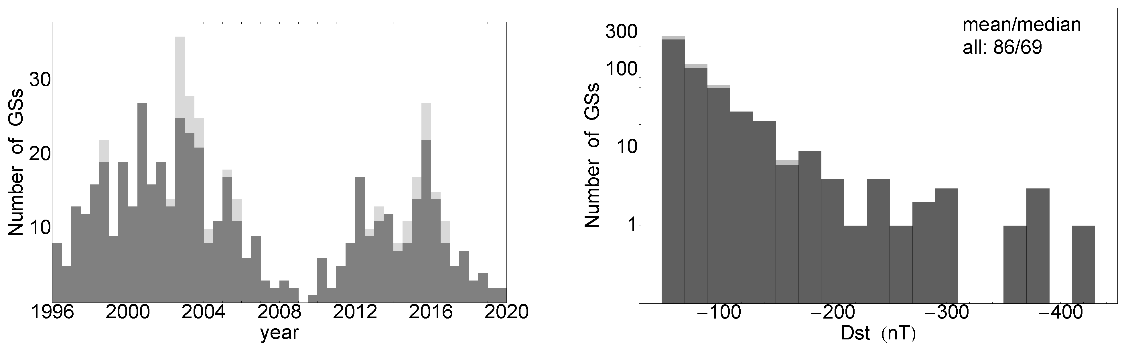
| GS |Dst| | 91/71 (361) | 75/66 (185) | 86/69 (546) |
| - certain | 92/72 (331) | 77/67 (166) | 87/70 (497) |
| - uncertain | 74/70 (30) | 65/57 (19) | 71/64 (49) |
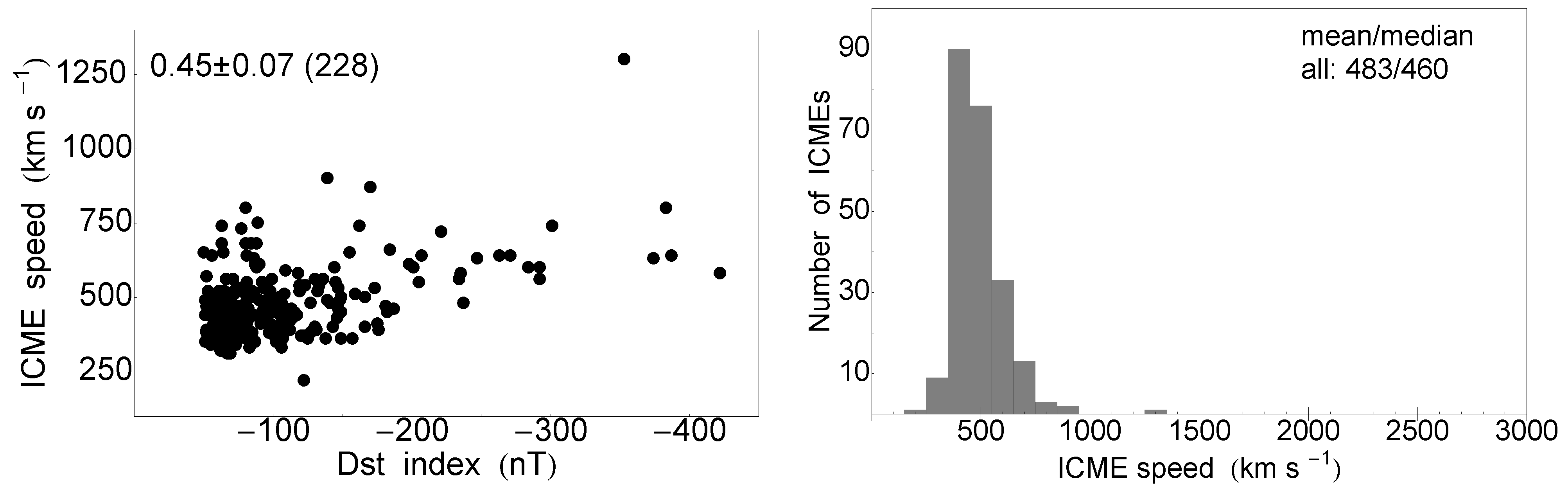
| ICME speed | 499/460 (159) | 447/440 (69) | 483/460 (228) |
| - certain | 495/460 (151) | 446/435 (68) | 480/450 (219) |
| - uncertain | 575/520 (8) | 490 (1) | 566/520 (9) |
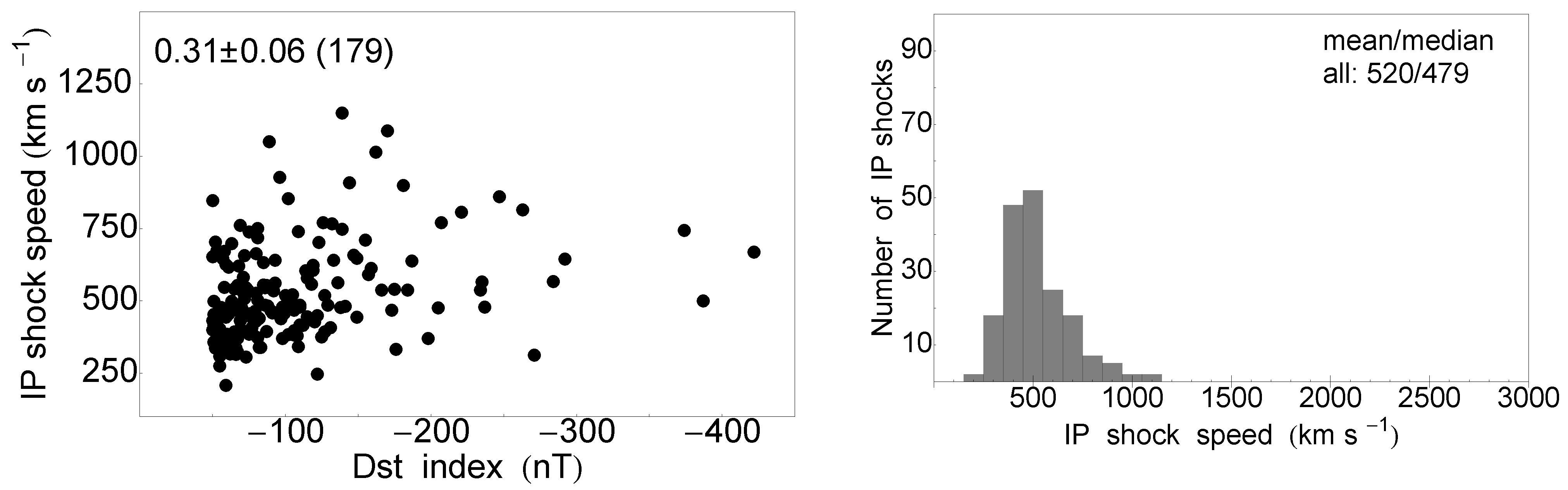
| IP shock speed | 543/517 (127) | 463/445 (52) | 520/479 (179) |
| - certain | 537/500 (124) | 463/440 (48) | 517/478 (172) |
| - uncertain | 787/768 (3) | 452/470 (4) | 595/497 (7) |
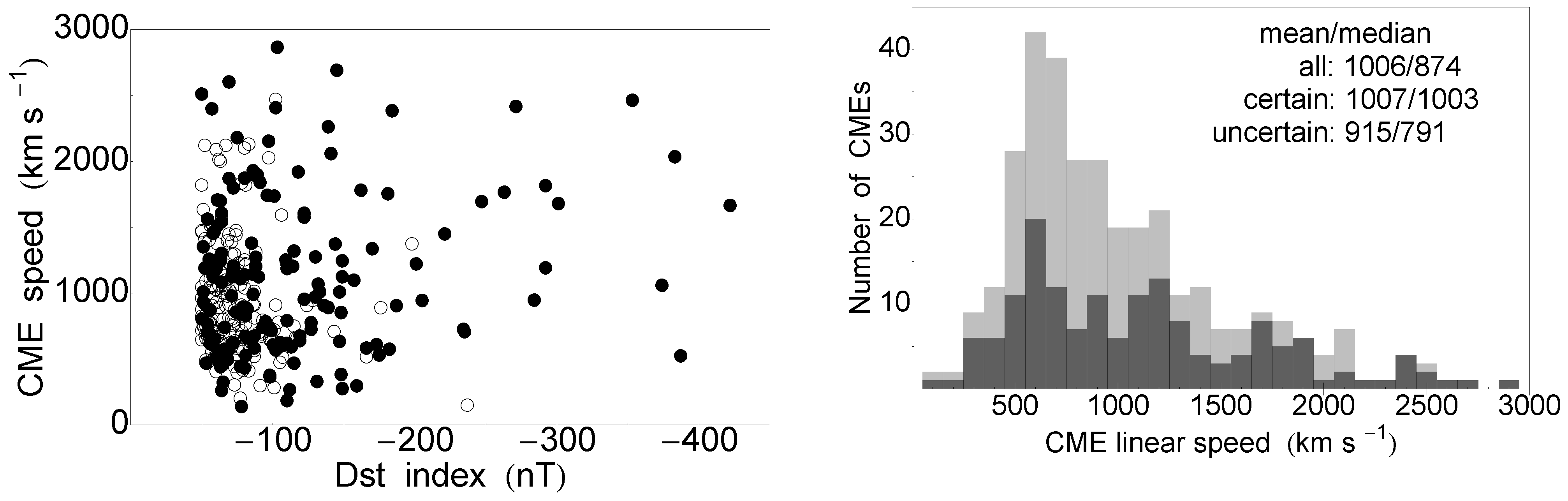
| CME speed | 1037/899 (220) | 943/803 (110) | 1006/874 (330) |
| - certain | 1123/1004 (114) | 2684/987 (43) | 1007/1003 (157) |
| - uncertain | 945/833 (106) | 866/745 (67) | 915/791 (173) |
| CME AW | 278/360 (220) | 286/360 (110) | 280/360 (330) |
| - certain | 331/360 (114) | 353/360 (43) | 337/360 (157) |
| - uncertain | 220/182 (106) | 243/257 (67) | 229/200 (173) |
| SF class | M1.5/M1.2 (157) | M1.5/M1.8 (70) | M1.5/M1.4 (227) |
| - certain | M3.1/M3.9 (86) | M2.1/M2.8 (32) | M2.8/M3.5 (118) |
| - uncertain | C6.4/C5.2 (71) | M1.1/M1.3 (38) | C7.7/C6.7 (109) |
| SEP flux | 0.71/0.61 (57) | 0.21/0.14 (33) | 0.45/0.31 (90) |
| - certain | 1.19/0.67 (43) | 0.35/0.39 (20) | 0.80/0.60 (63) |
| - uncertain | 0.14/0.16 (14) | 0.10/0.07 (13) | 0.12/0.10 (27) |
| SEE flux | 7.8/9.8 (69) | 2.1/1.3 (41) | 4.8/4.6 (110) |
| - certain | 13.5/12.4 (51) | 2.9/1.3 (23) | 8.4/9.5 (74) |
| - uncertain | 1.7/1.2 (18) | 1.4/1.0 (18) | 1.5/1.2 (36) |
Disclaimer/Publisher’s Note: The statements, opinions and data contained in all publications are solely those of the individual author(s) and contributor(s) and not of MDPI and/or the editor(s). MDPI and/or the editor(s) disclaim responsibility for any injury to people or property resulting from any ideas, methods, instructions or products referred to in the content. |
© 2023 by the authors. Licensee MDPI, Basel, Switzerland. This article is an open access article distributed under the terms and conditions of the Creative Commons Attribution (CC BY) license (https://creativecommons.org/licenses/by/4.0/).
Share and Cite
Miteva, R.; Samwel, S.W. Catalog of Geomagnetic Storms with Dst Index ≤ −50 nT and Their Solar and Interplanetary Origin (1996–2019). Atmosphere 2023, 14, 1744. https://doi.org/10.3390/atmos14121744
Miteva R, Samwel SW. Catalog of Geomagnetic Storms with Dst Index ≤ −50 nT and Their Solar and Interplanetary Origin (1996–2019). Atmosphere. 2023; 14(12):1744. https://doi.org/10.3390/atmos14121744
Chicago/Turabian StyleMiteva, Rositsa, and Susan W. Samwel. 2023. "Catalog of Geomagnetic Storms with Dst Index ≤ −50 nT and Their Solar and Interplanetary Origin (1996–2019)" Atmosphere 14, no. 12: 1744. https://doi.org/10.3390/atmos14121744