Dimensional Transitions in Turbulence: The Effects of Rotation and Stratification

Abstract

The transition from two-dimensional to three-dimensional turbulence is a fascinating problem which finds applications in the study of geophysical flows. This paper briefly reviews the research in this field with emphasis on the role of rotation and stratification, two important ingredients of geophysical flows at large scales. By means of direct numerical simulations of the Navier–Stokes equations, the conditions for the emergence of a split cascade, with a simultaneous cascade of energy to both the large and the small scales, are discussed.

1. Introduction

Geophysical flows at large scales can often be considered as quasi-two-dimensional (2D). While this is evident from a geometrical point of view, the effects of confinement on the dynamics of the flow are less obvious, since the confinement is much larger than the dissipative viscous scales and the flow is intrinsically three-dimensional (3D). Strictly speaking, no real flow is two-dimensional. Nonetheless, when one considers a very thin layer of fluid, one can safely assume that both the vertical velocity and the vertical dependence of the fields are suppressed and the flow can be described by the 2D version of the Navier–Stokes equation. We recall that the main difference between the 3D and the 2D versions is the absence, for the latter, of the vortex stretching term which is responsible for the non-conservation (and the amplification) of vorticity [1]. As a consequence, in two dimensions the enstrophy (average square vorticity) is an inviscid invariant together with the kinetic energy (average square velocity), and this prevents the viscous dissipation of kinetic energy at small scales, which therefore flows to the large scales, producing the inverse cascade.

Turbulent flows in quasi-2D geometries exhibit a rich and interesting phenomenology which has stimulated several studies. Numerical simulations [2,3,4] and laboratory experiments [5,6] have shown that, by changing the confinement, 2D and 3D phenomenologies coexist in a range of parameters with the simultaneous presence of an inverse and a direct cascade of energy. The key parameter which controls the relative flux of the two cascades is the ratio S between the confining scale and the characteristic forcing scale at which energy is injected. In particular, it has been found that there exists a critical ratio $S_c$ above which the inverse cascade vanishes and the turbulent flow fully recovers the 3D phenomenology [2]. We remark that in particular conditions, such as the presence of a large-scale vortex, this transition can become more complex and displays bistability and hysteresis [7,8].

The dimensional transition, and in particular the critical value $S_c$, is affected by other physical ingredients, including rotation [9,10] and stratification, the presence of a magnetic field, or more exotic features [11]. A rotation of the flow in the direction of confinement in general favors bidimensionalization, i.e., boosts the inverse flux with respect to the non-rotating case at fixed S, and increases the critical value $S_c$. Conversely, the presence of a stable stratification of the density field in the Boussinesq approximation reduces the inverse energy flux and therefore decreases the critical value $S_c$. In this paper, we will review the dimensional transition in turbulent flows both induced by spatial confinement alone and with the presence of rotation or stratification. The results presented are obtained on the basis of extensive direct numerical simulations of the Navier–Stokes–Boussinesq model.

Jack Herring made fundamental and pioneering contributions in the study of two-dimensional turbulence by comparing the statistical theories with direct numerical simulations and recognizing the physical origin of the discrepancies observed in the direct cascade of enstrophy [12] and its non-universality with respect to the forcing statistics [13], highlighting one important difference between 2D and 3D turbulence. Remarkably, in an important paper in 1989, Herring also observed the emergence of an inverse cascade in a forced, stably stratified three-dimensional turbulent flow [14], thus anticipating by many years the systematic studies of dimensional transition in turbulence which is the subject of this contribution.

The remaining part of the paper is organized as follows. Section 2 introduces the mathematical model and the relevant dimensionless number of the problem, while in Section 3, we report the results of numerical simulations. Section 4 is devoted to the conclusions.

2. Mathematical Models

We consider, in general, an incompressible flow in the presence of a stable stratification in the (vertical) direction of the acceleration $\mathit{g}=(0,0,-g)$ with a constant density gradient $\gamma$ and in a frame of reference rotating with constant angular velocity $\mathbf{\Omega }=(0,0,\mathrm{\Omega })$. The flow is confined in a box of volume $V=L_x\times L_y\times L_z$, and, in order to preserve homogeneity, periodic boundary conditions are imposed in all the directions. In the Boussinesq approximation, the equation of motion for the velocity field $\mathit{u}(\mathit{x},t)$ and the density $\varphi (\mathit{x},t)$ are, respectively,

$${\partial }_t\mathit{u}+\mathit{u}·\mathbf{\nabla }\mathit{u}+2\mathbf{\Omega }\times \mathit{u}=-\frac{1}{{\rho }_0}\mathbf{\nabla }p+\nu {\nabla }^2\mathit{u}-N\varphi {\mathit{e}}_3+\mathit{f}$$

(1)

$${\partial }_t\varphi +\mathit{u}·\mathbf{\nabla }\varphi =\kappa {\nabla }^2\varphi +N{\mathit{e}}_3·\mathit{u}$$

(2)

together with the incompressibility condition $\mathbf{\nabla }·\mathit{u}=0$. In (1), $\nu$ is the kinematic viscosity, $\kappa$ is the scalar diffusivity, and $N=\sqrt{\gamma g/{\rho }_0}$ is the Brunt–Väisäla frequency associated with the stratification. The field $\varphi$ has the dimension of a velocity and is proportional to the deviation of the density field from the linear stable profile, $\rho ={\rho }_0+\gamma (\varphi /N-z)$. The flow is sustained by the external forcing $\mathit{f}(\mathit{x},t)$, which is a stochastic Gaussian, white in time noise, active only on the horizontal components $u_x$, $u_y$ of the velocity, and depends on the horizontal components x, y only. The forcing is localized in Fourier space in a narrow band of wave numbers around $k_f=2\pi /L_f$ and injects energy into the system at a fixed rate ${\epsilon }_I$ [15].

The relevant dimensionless parameters are the thickness numbers

$$S=\frac{L_z}{L_f}$$

(3)

which quantify the vertical confinement with respect to the forcing scale, the Froude number

$$Fr=\frac{{\left(k_f^2{\epsilon }_I\right)}^{1/3}}{N}$$

(4)

ratio of the forcing frequency to the Brunt–Väisäla frequency, and the Rossby number

$$Ro=\frac{{\left(k_f^2{\epsilon }_I\right)}^{1/3}}{\mathrm{\Omega }}$$

(5)

which is the ratio of the characteristic frequency at the forcing scale to the rotation rate. We remark that, since the flow has periodic boundary conditions, the effect of a finite $L_z$ is that just of reducing the number of modes available in the z direction. Different boundary conditions, such as those present in laboratory experiments, can change quantitatively the results [16]. We also remark that the horizontal scales $L_x$ and $L_y$ are assumed to be much larger than the other scales, and they will not play any role in the dynamics.

In the absence of forcing and dissipation, (1) and (2) conserve the total energy density, given by the sum of kinetic and potential contributions

$$E=E_k+E_p=\frac{1}{2}{\langle \left|\mathit{u}\right|}^2\rangle +\frac{1}{2}\langle {\varphi }^2\rangle$$

(6)

where $\langle \dots \rangle \equiv \frac{1}{V}\int d^{3}x$ represents the average over the domain of volume V. From (1) and (2), the balances of kinetic and potential energy can be written as

$$\frac{d{E}_k}{dt}\equiv {\epsilon }_{\alpha }={\epsilon }_f-{\epsilon }_{\nu }-{\epsilon }_x$$

(7)

$$\frac{d{E}_p}{dt}={\epsilon }_x-{\epsilon }_{\kappa }$$

(8)

where ${\epsilon }_{\nu }=\nu \langle {\partial }_i{u}_j{\partial }_i{u}_j\rangle$ (summation over repeated indices is assumed) is the viscous dissipation rate and ${\epsilon }_{\kappa }=\kappa \langle {\partial }_i\varphi {\partial }_i\varphi \rangle$ is the diffusive dissipation rate. By introducing the vorticity field $\mathit{\omega }=\mathbf{\nabla }\times \mathit{u}$, the viscous dissipation can be written ad ${\epsilon }_{\nu }=2\nu Z$, where $Z=\langle |\mathit{\omega }{|}^2\rangle /2$ is the enstrophy. The term ${\epsilon }_x=N\langle u_3\varphi \rangle$ represents the exchange rate between kinetic and potential energies. Although the sign of this exchange rate is not defined a priori, the analysis of the Kármán–Howarth–Monin equations shows that it is positive on average [17]. This indicates that part of the kinetic energy is converted to produce potential energy in the flow, which is eventually dissipated by the last term in (8). In the presence of an inverse cascade, the flow displays a long non-stationary transient with the energy being transferred to large scales. Eventually the energy reaches the largest scale (the box size) and starts to accumulate until the amplitude of this mode saturates by the dissipation induced by viscosity [18,19]. Since in a turbulent flow the Reynolds number (inverse of viscosity) is large, this effect appears for a very long time only, and the rate ${\epsilon }_{\alpha }$ of energy growth during this long transient is therefore used as a measure of the strength of the inverse cascade.

Direct numerical simulations of the models (1) and (2) are performed in a box of dimension $L_x=L_y$ and $L_z$ discretized on a uniform grid at resolution $N_x\times N_y\times N_z$ by a fully parallel pseudospectral code, with a standard $2/3$ dealiasing scheme. Most of the results are obtained at a resolution $N_x=N_y=512$ and $N_z=S{N}_x/8$ with $S=L_z/L_f$ ranging from $S=0.25$ to $S=8.0$ and forcing wavenumber $k_f=8$. For the non-rotating, non-stratified case we use also data from a simulation at $N_x=N_y=4069$ and $N_z=64$ with $k_f=16$. For rotating turbulence, we analyze six simulations at Rossby number $Ro=0.1,0.2,0.67,1.0,1.33,2.0$, while for the stratified flow we have eight different Froude numbers $Fr=0.15,0.2,0.25,0.3,0.4,0.5,0.6,0.75$. In all the simulations, the viscous and the diffusive terms are replaced by a hyperviscous damping scheme of higher order [20]. More details on the numerical simulations can be found in [17,20,21].

3. Numerical Results

3.1. Transition in the Absence of Rotation and Stratification

The simplest case is when rotation and stratification can be neglected. Formally, this corresponds to having ${Ro}^{-1}=F{r}^{-1}=0$ (in terms of the physical parameters $\mathrm{\Omega }=0$ and $N=0$). In this limit, (2) decouples from (1): $\varphi$ becomes a passive scalar which can be neglected since it does not affect the dynamics. The thickness scale controls the fate of the energy injected in the flow at the scale $L_f$. Extensive numerical simulations [2,4,20] complemented with laboratory experiments [5,6] show that when the thickness is large ($S>1$), the flow develops a 3D motion at the injection scale and energy is transferred to small scales by a direct cascade, as in the usual 3D turbulence. In the limit of small $S\ll 1$, the flow becomes essentially two-dimensional (i.e., vertical motions are suppressed) and an inverse cascade of energy is observed [22]. Remarkably, for intermediate values of the thickness number, one observes a split cascade with a fraction of the injected energy going to the large scales and the remaining energy flowing to small scales. In this regime, the fraction of energy flowing to large/small scales is controlled by the parameter S.

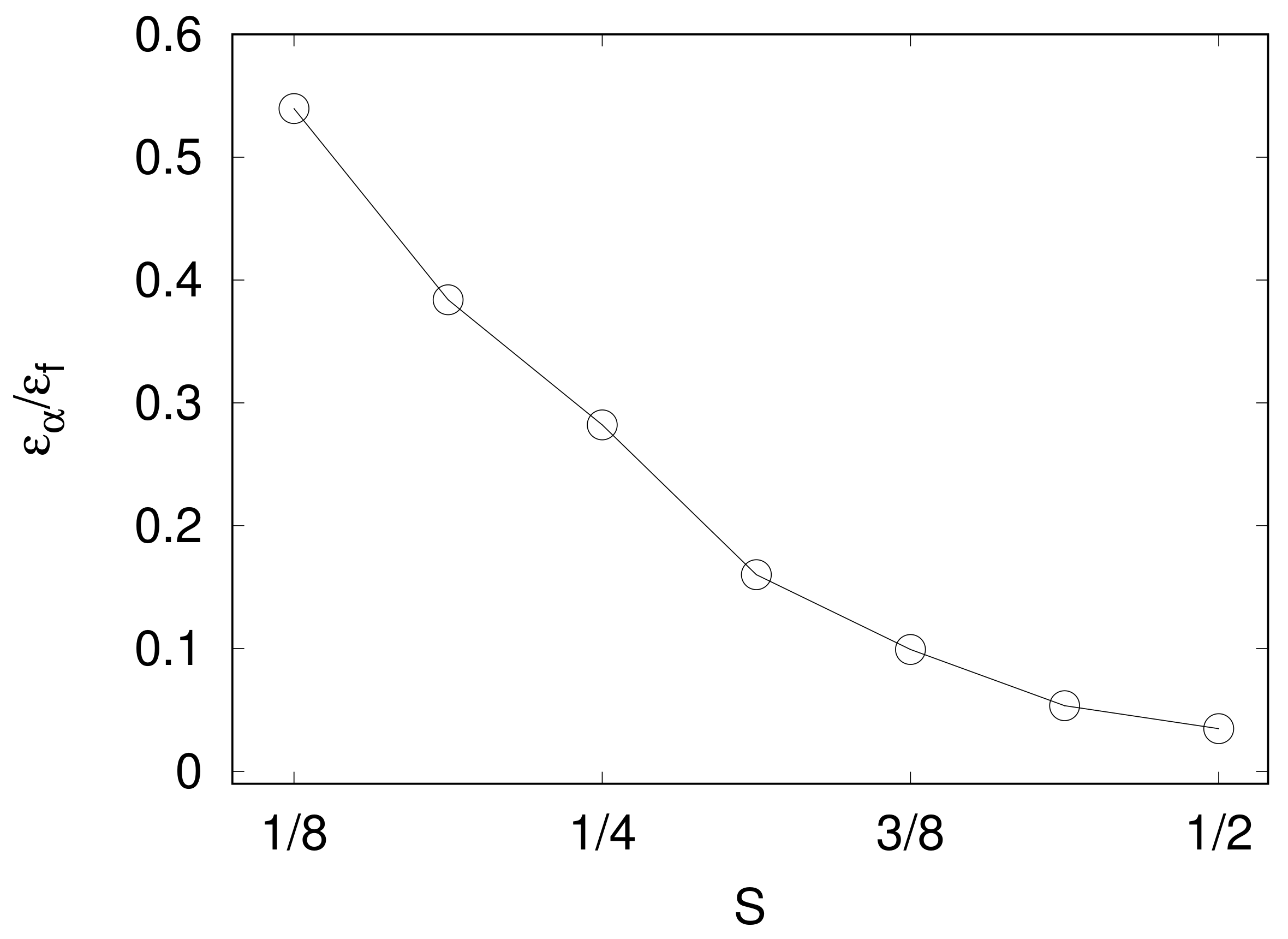
Figure 1 shows the fraction of energy transferred to large scales (i.e., the rate of kinetic energy growth), which quantifies the strength of the inverse cascade as a function of S from direct numerical simulations of a thin layer of fluid. As shown in similar works [4] for $S\ge S_c\simeq 1/2$, the inverse cascade disappears and all the energy flows to small scales where it is dissipated by viscosity. As shown by Figure 1, for $S=1/8$, about one-half of the kinetic energy is transferred to the large scales.

We remark that the threshold $S_c=1/2$ is not expected to be a universal value as it depends on the details of the forcing and also on the precise definition of $L_f$. Indeed, different forcing schemes lead to different values of $S_c$ at which the inverse flux vanishes [2,23].

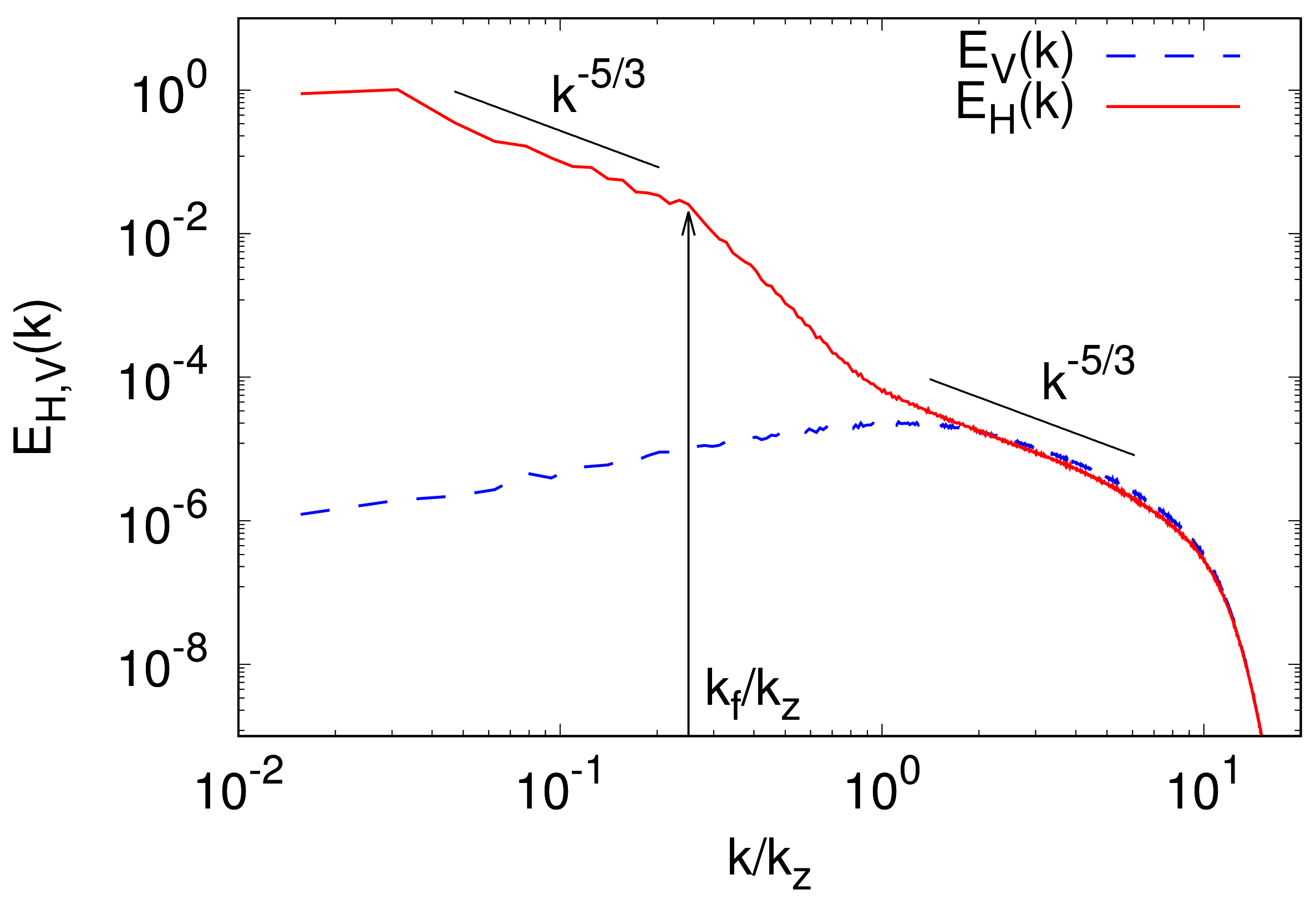
The kinetic energy spectrum in the split cascade regime at $S=1/4$ is shown in Figure 2. The spectrum is computed at a late time when the inverse cascade is well developed and we are able to observe the presence of three different scaling laws. Only the two horizontal components of the velocity are used to compute the spectrum, and the wavenumber is restricted to the horizontal wavenumber $k={(k_x^2+k_y^2)}^{1/2}$ on the plane $k_z=0$. This is equivalent to the spectrum of the velocity field averaged over the vertical direction z.

At large scales, $k<k_f$, we clearly see the inverse energy cascade with Kolmogorov scaling $k^{-5/3}$ [24]. At intermediate scales, $k_f<k<k_z$, we observe a steeper spectrum, compatible with a direct enstrophy cascade. Finally, for $k>k_f$, the flow becomes three-dimensional, and a direct energy cascade, again with Kolmogorov scaling, is observed. We remark that the intermediate, enstrophy cascade, spectrum is expected in a narrow range of wavenumbers with ratio $k_z/k_f=1/S$. Figure 2 also shows the spectrum of the vertical component of the velocity. This is strongly suppressed at large scales, but it reaches the horizontal spectrum at $k\ge k_z$, an indication of the recovery of isotropy at small scales.

In order to better understand the phenomenology of the split cascade, it is useful to consider the vorticity equation, obtained by taking the curl of (1):

$${\partial }_t\mathit{\omega }+\mathit{u}·\mathbf{\nabla }\mathit{\omega }=\mathit{\omega }·\mathbf{\nabla }\mathit{u}+\nu {\nabla }^2\mathit{\omega }{\mathit{f}}_{\omega }$$

(9)

where ${\mathit{f}}_{\omega }=\mathbf{\nabla }\times \mathit{f}$. As discussed in the Introduction, in two-dimensions the vortex stretching term in (9) identically vanishes, and therefore, in that case the enstrophy is a second inviscid invariant. This is the main difference with respect to 3D turbulence where the vortex stretching term is responsible for the increase in enstrophy which dissipates the energy flowing to small scales.

In the case considered here, the flow is three-dimensional, and therefore enstrophy is not expected to be conserved. Nonetheless, the appearance of a 2D-like phenomenology suggests that, at large scales, the vortex stretching terms are dynamically suppressed and therefore the “large scale enstrophy” is conserved. In order to quantify this effect, we compute the different contributions to the enstrophy flux. By taking the Fourier transform of (9) and multiplying by ${\widehat{\mathit{\omega }}}^{*}$ (the conjugate of the Fourier transform), we define

$${\mathrm{\Pi }}_Z\left(k\right)={\int }_{\left|\mathit{q}\right|\le k}{\widehat{\mathit{\omega }}}^{*}\left(\mathit{q}\right)\widehat{(\mathit{u}·\mathbf{\nabla }\mathit{\omega })}\left(\mathit{q}\right)d\mathit{q}$$

(10)

as the enstrophy flux and

$${\mathrm{\Sigma }}_Z\left(k\right)={\int }_{\left|\mathit{q}\right|\le k}{\widehat{\mathit{\omega }}}^{*}\left(\mathit{q}\right)\widehat{(\mathit{\omega }·\mathbf{\nabla }\mathit{u})}\left(\mathit{q}\right)d\mathit{q}$$

(11)

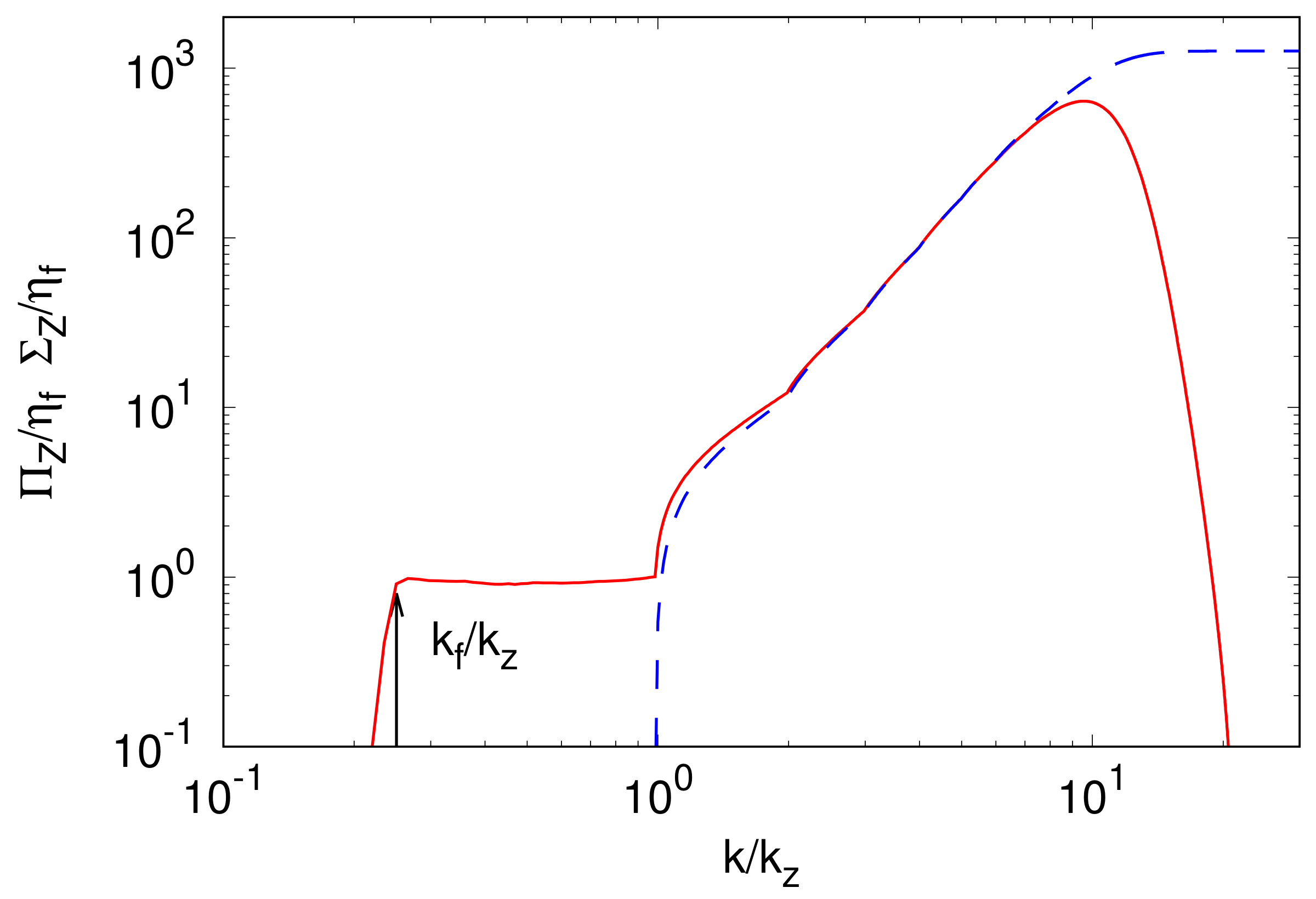
as the spectral enstrophy production. While ${\mathrm{\Pi }}_Z\left(k\right)$ represents the transport of enstrophy across the wavenumber k by the nonlinear (advection) term, ${\mathrm{\Sigma }}_Z\left(k\right)$ is the generation of enstrophy at wavenumbers smaller than k due to the vortex stretching mechanism. The results from the simulation are shown in Figure 3. For wavenumber $k<k_f$, in the region of the inverse energy cascade, both the enstrophy flux and production are close to zero, as in the 2D case. In the intermediate range of wavenumber $k_f<k<k_z$, the production of enstrophy (i.e., the vortex stretching term) is still negligible while the flux is constant, as in a 2D direct enstrophy cascade. At large wavenumbers $k>k_z$, the production of enstrophy becomes significant, and therefore the flux is not constant anymore but grows following the production term.

The fact that enstrophy behaves at large scales as a quasi-invariant is remarkable since it indicates that the development of the inverse energy cascade is not caused by the two-dimensionalization of the flow but by the presence of a second sign-definite conserved quantity at large scales. The development of an inverse energy cascade due to the presence of a second inviscid invariant has been observed also in other turbulent systems, e.g., in a homogeneous isotropic 3D flow with mirror symmetry broken such that helicity has a well-defined sign at all wave numbers [25].

3.2. Dimensional Transition in Rotating Turbulence

We now consider how the phenomenology described in the previous section changes in the presence of rotation. To this aim we consider the case of finite Rossby number $Ro$ in the limit of infinite Froude number $Fr$. This corresponds to integrating (9) with $N=0$ and $\mathrm{\Omega }>0$. The results of this section are to a large extent presented in [21].

It is well known that rotation in general favors the two-dimensionalization of the flow, and the Taylor–Proudman theorem supports this idea. In turbulent flows, the onset of an inverse cascade in the presence of rotation has been observed in laboratory experiments [26,27]. However, it is not obvious how, starting from a 3D turbulent flow, the actual two-dimensionalization would occur. Different mechanisms have been proposed, including (nearly) resonant triad interactions [28,29] and weak turbulence theory [30,31].

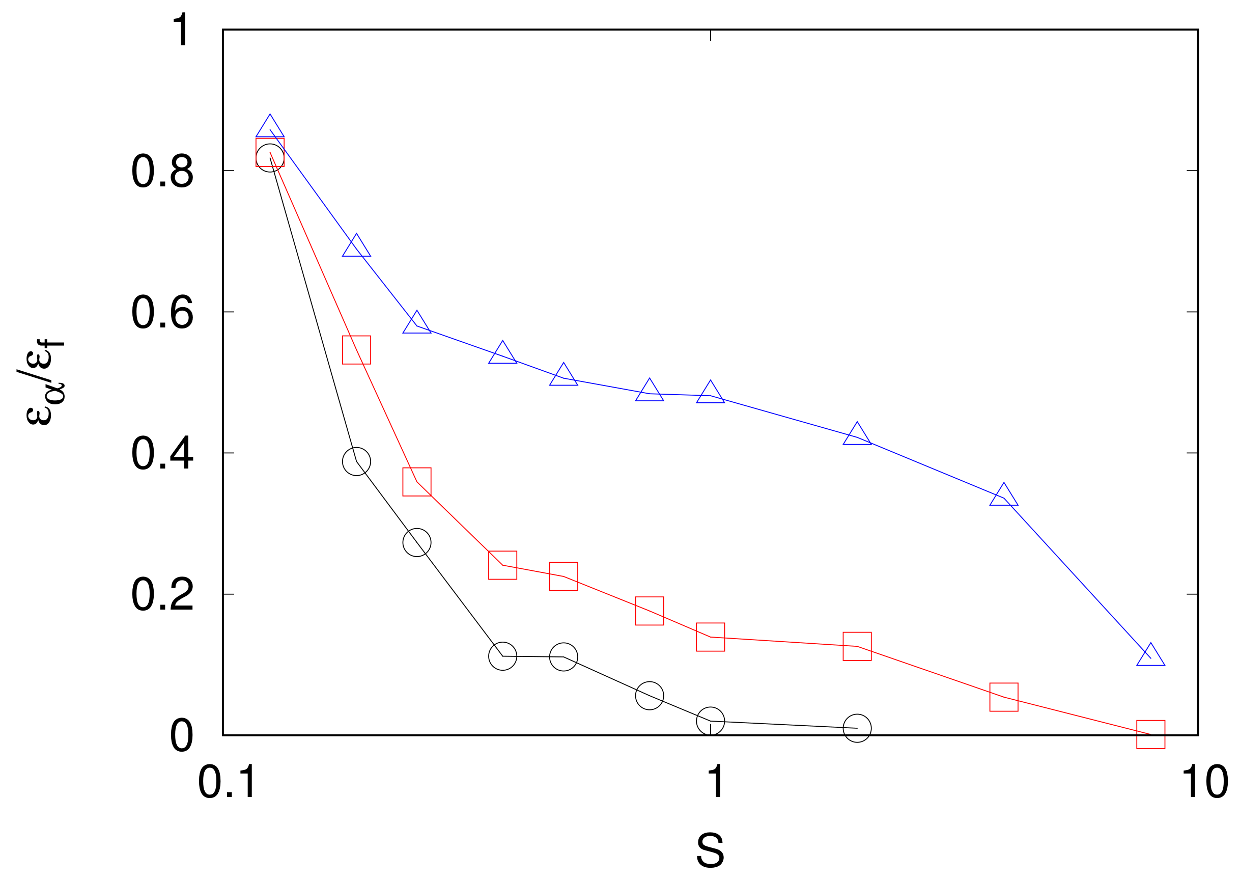
In the presence of confinement, it has been observed that a moderate rotation enhances the fraction of energy which is transferred to large scales and that the split cascade survives also for $S>1/2$ [21]. Figure 4 displays the fraction of energy transferred to large scale for different Rossby numbers. We observe that indeed ${\epsilon }_{\alpha }$ increases by decreasing $Ro$ and that, for the strongest rotation (smallest $Ro$), a residual inverse cascade is present even for $S=10$. We remark that this result is consistent with the observation, based on asymptotic techniques, that for sufficiently rapid rotation, the dimensional transition persists for large S [10]. Moreover, in the limit of strong rotation it can be shown that 2D turbulence is stable to vertically dependent perturbations [32,33]. In the case of fast rotation, it has been shown that the inverse cascade is also sustained by the interaction among triads with the same sign of helicity [34]. From the data in Figure 4, it is evident that $S_c$ is a decreasing function of $Ro$.

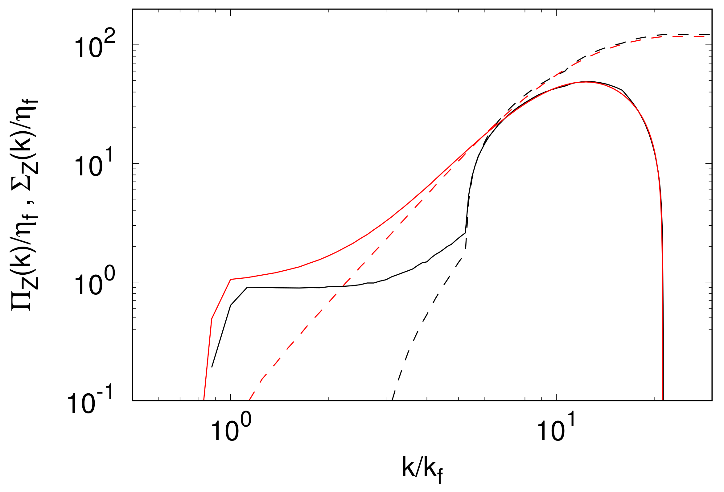
Figure 5 shows the spectral enstrophy flux and the enstrophy production for a non-rotating ($Ro\to \infty$) simulation at $S=0.188$ and a simulation with $Ro=2/3$ and $S=4$. By comparing Figure 1 and Figure 4, we see that the two flows have approximatively the same ratio between the inverse and direct energy fluxes, and therefore it is interesting to compare whether this is due to the same mechanism. Figure 5 shows that this is not the case. As discussed in the previous section, in the non-rotating case (black lines) the vortex stretching contribution to the flux is completely suppressed for $k<k_z$, and a direct cascade with an almost constant flux of enstrophy is observed for $k_f<k<k_z$. In the case of rotating turbulence (red lines), we observe that the suppression of the vortex stretching term is less sharp, and, consequently, there is no evidence of a direct cascade of enstrophy with a constant flux. This suggests that a different mechanism for the split cascade is at work in this case. In spite of these differences, it is interesting to observe that at small scales the enstrophy production and the enstrophy flux of the two cases become indistinguishable.

3.3. Cyclonic-Anticyclonic Asymmetry in a Thin Layer

One of the distinctive features of rotating turbulence is the breakdown of the symmetry between cyclonic (i.e., rotating in the direction of $\mathbf{\Omega }$) and anticyclonic vortices, i.e., an asymmetric distribution of the vorticity ${\omega }_z$ with a predominance of positive values. This feature has been observed in many experiments and numerical simulations [35,36,37,38,39,40], both in forced and decaying turbulence. Nonetheless, the origin of the asymmetry is still not fully understood, and different types of arguments have been proposed to explain the phenomenon [41,42]. A simple, natural way to quantify the asymmetry of ${\omega }_z$ is by computing the skewness of its distribution

$$Sk=\frac{\langle {\omega }_z^3\rangle }{{\langle {\omega }_z^2\rangle }^{3/2}}.$$

(12)

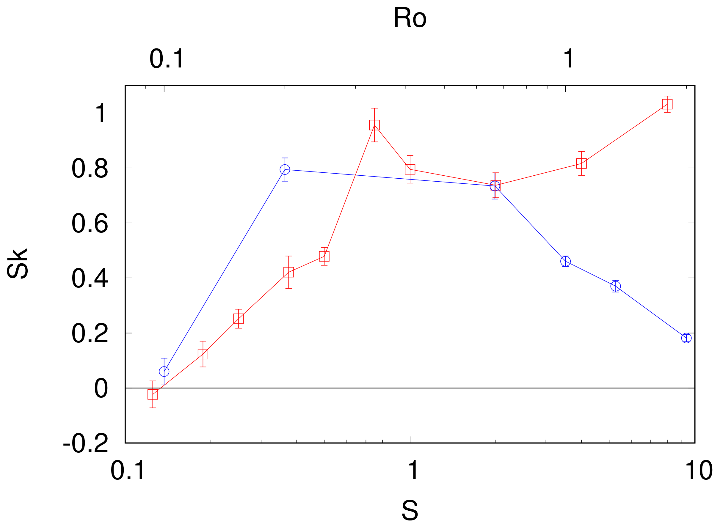
It is interesting to study how this asymmetry, due to the background rotation of the flow, is influenced by the confinement in the direction of rotation. Indeed, in the limit of a two-dimensional flow, $S\to 0$, rotation cannot induce an asymmetry in the distribution of ${\omega }_z$ since in this case the Coriolis term $\mathbf{\Omega }\times \mathit{u}$ disappears in the 2D version of (9). The dependence of $Sk$ on the confinement S for a turbulent flow rotating with $Ro=2/3$ is shown in Figure 6. We observe that indeed $Sk\to 0$ at small S, as expected for a purely 2D flow. For $S>1$, the numerical indication is that the skewness saturates at a value $Sk\simeq 1$, at least in the range of confinement studied. We remark that for all these values of S, an inverse cascade is present in the flows, as shown by Figure 4.

Figure 6 also shows the dependence of $Sk$ on the Rossby number. We observe that in this case, the behavior is non-monotonic with a maximum of asymmetry for intemediate values of $Ro$.

3.4. Dimensional Transition in Stably Stratified Flows

In this section, we consider the effect of a stable density stratification on the dimensional turbulent transition in a thin layer. We recall that stably stratified flows occur naturally in many instances of geophysical flows, both in the ocean and in the atmosphere. Therefore, many laboratory experiments and numerical simulations have been devoted to the study of stratified turbulence [43,44,45]. In particular, we remark that early numerical simulations of stratified turbulence reported the existence of an inverse cascade [14], while other simulations have observed a direct cascade [46,47], in particular in the limit of strong stratification [48,49].

From these considerations, it is therefore interesting to study how stratification affects the dimensional transition in a thin turbulent layer and in particular how critical thickness $S_c$ observed in non-stratified flows is affected. This problem has been addressed on the basis of extensive direct numerical simulations of the models (1) and (2) with $\mathbf{\Omega }=0$ and for different values of the Froude number $Fr$ and of the thickness number S. We remark that the two limits of thin layer $S\to 0$ and of strong stratification $Fr\to 0$ are not expected to commute. In particular, if the limit $Fr\to 0$ is taken first, one cannot expect that the 2D limit is recovered when $S\to 0$ [17].

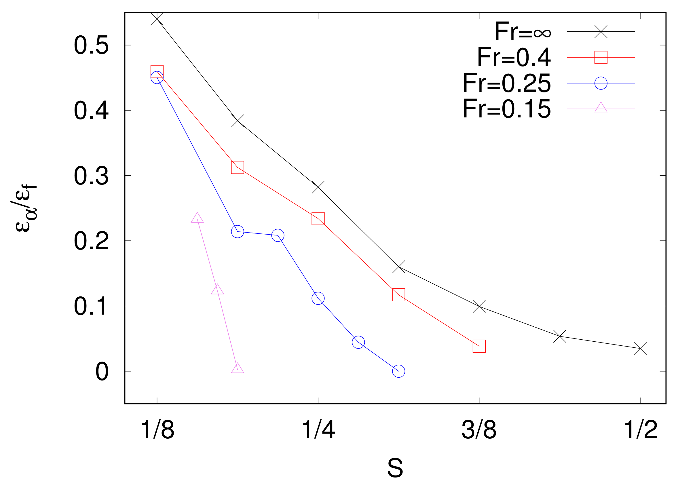
For each simulation at given values of the parameters $(Fr,S)$, the growth rate of kinetic energy is measured and used, according to (7), as a proxy for the inverse energy flux ${\epsilon }_{\alpha }$. As shown in Figure 7, for each value of the stratification parameter $Fr$, the ratio ${\epsilon }_{\alpha }/{\epsilon }_f$ is a decreasing function of the thickness number S. This indicates that the presence of a stable stratification in the flow reduces the intensity of the inverse cascade.

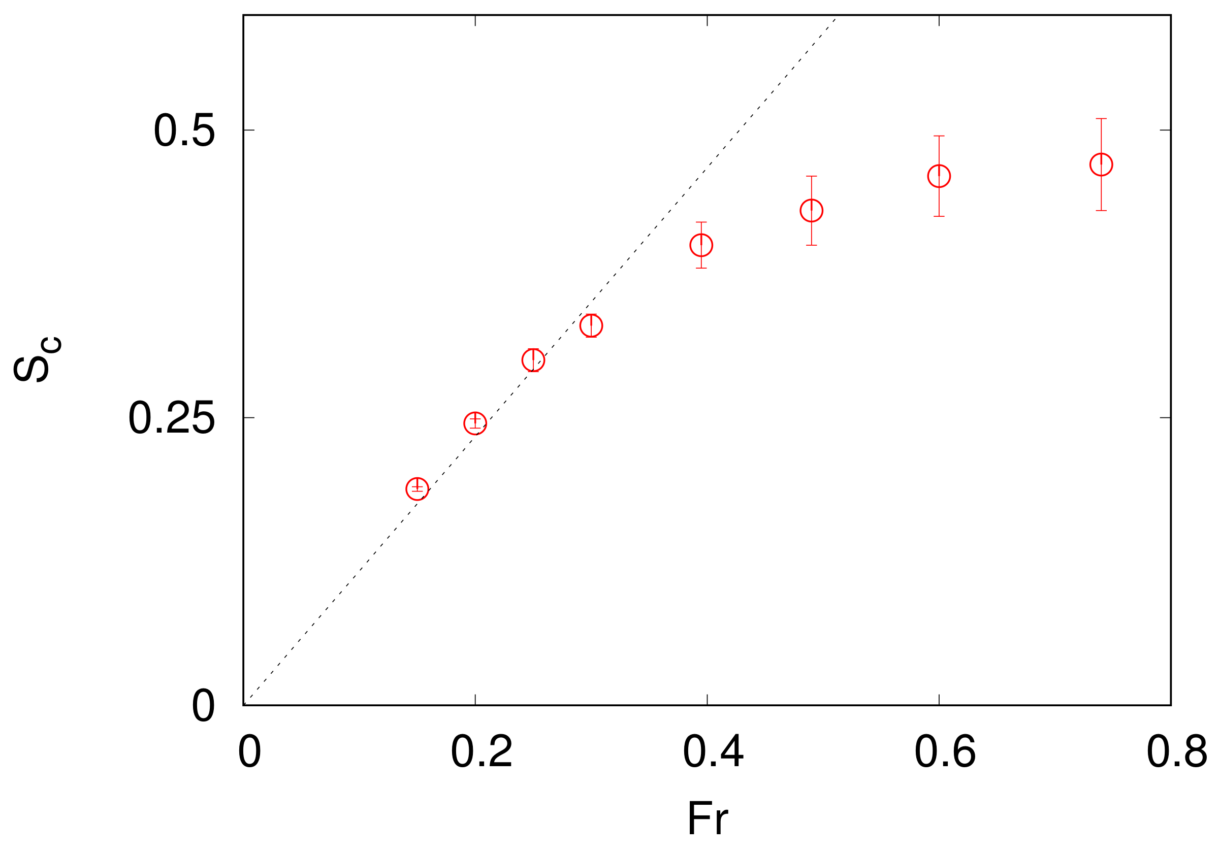
The inverse flux is found to vanish at the critical thickness $S_c\left(Fr\right)$, which becomes smaller as the stratification increases. The critical value is bounded by the value in the absence of stratification, $S_c\left(Fr\right)\le S_c(\infty )\simeq 1/2$. Figure 8 shows the critical value $S_c$ as a function of the Froude number. For strong stratification, we observe approximatively a linear behavior $S_c\sim Fr$. A geometrical interpretation of this behavior is the following [17]. By introducing the characteristic vertical scale of the layered structures which characterize a stratified flow $L_v\simeq {\epsilon }_f^{1/3}{L}_f^{1/3}/N$ [49], one has

$$Fr=\frac{{\epsilon }_f^{1/3}{L}_f^{-2/3}}{N}=\frac{L_v}{L_f}=\frac{L_v}{L_z}S$$

(13)

The behavior seen in Figure 8 $S_c\simeq Fr$ corresponds to $L_v\simeq L_z$ and therefore suggests that the inverse cascade is suppressed when the typical thickness of the layered structure becomes small enough to fit in the fluid layer. In this case, the kinetic energy injected at $L_f$ is converted into potential energy by the term ${\epsilon }_x$ in (7) and is eventually dissipated at small scales according to (8) [17].

The analysis of spectral fluxes of both kinetic and potential energy confirms this picture. Indeed, by increasing the stratification at fixed S, the inverse flux of kinetic energy is reduced (as shown in Figure 7), while the direct flux of energy is enhanced in the range of wavenumber $k_f<k<k_z$ (remember that, since $S<1$, $k_z>k_f$). For $k>k_z$, the analysis of fluxes shows the development of a cascade of potential energy which subtracts kinetic energy at large wavenumbers. This process is activated when the thickness of the vertical structures $L_v$ becomes smaller than $L_z$, and therefore the suppression of the inverse flux is expected to be proportional to $Fr$, as shown in Figure 8. It is interesting to observe that the scaling shown in Figure 8 for small $Fr$ can be extended to the fluctuations of the vertical velocity. Indeed, by incompressibility, one can write $u_z\simeq u_x{L}_v/L_x$, and therefore (13) implies that $u_z\propto Fr$ for small Froude numbers. This scaling was already observed in a remarkable paper by Herring on numerical simulations of stratified turbulence [14].

4. Conclusions

This paper briefly reviewed the recent studies on the transition between 2D and 3D turbulence in a confined thin fluid layer in the presence of rotation or a stable density stratification. It has been shown that confinement and rotation produce an inverse cascade of energy by a similar mechanism which suppresses enstrophy production at large scales. The presence of a density stratification, on the contrary, reduces the intensity of the inverse cascade and the critical thickness at which the inverse flux vanishes.

A natural extension of the studies reported here is to include both rotation and stratification in the fluid layer as it occurs in the oceans and in the atmosphere. Extensive studies in this direction have shown that stratification helps rotation to transfer energy to the two-dimensional modes [47,50] and, in particular conditions, can develop a Kolmogorov-like spectrum [51]. Moreover, numerical simulations of the 3D Boussinesq equation in the presence of both rotation and a stable stratification have shown that a small-scale energy flux can coexist with a large scale dynamics dominated by quasigeostrophic motion [52]. The key parameter which controls the ratio between large-scale and small-scale fluxes is the ratio $Ro/Fr$ [44,53], and this ratio is found to be close to that estimated for the ocean when using realistic values of the parameters [54]. These, together with other studies in recent years [55,56,57,58], have achieved at least a partial understanding of the complex phenomenology which emerges when turbulence is coupled with the fundamental physical ingredients of geophysical flows (confinement, rotation, and stratification). These results are therefore an important guide for the analysis of more complex models for the atmosphere and the oceans.

References

- Frisch, U. Turbulence: The Legacy of AN Kolmogorov; Cambridge University Press: Cambridge, UK, 1995. [Google Scholar]
- Smith, L.; Chasnov, J.; Waleffe, F. Crossover from Two- to Three-Dimensional Turbulence. Phys. Rev. Lett. 1996, 77, 2467–2470. [Google Scholar] [CrossRef] [PubMed]
- Ngan, K.; Straub, D.; Bartello, P. Aspect ratio effects in quasi-two-dimensional turbulence. Phys. Fluids 2005, 17, 125102. [Google Scholar] [CrossRef]
- Celani, A.; Musacchio, S.; Vincenzi, D. Turbulence in more than two and less than three dimensions. Phys. Rev. Lett. 2010, 104, 184506. [Google Scholar] [CrossRef] [PubMed]
- Xia, H.; Byrne, D.; Falkovich, G.; Shats, M. Upscale energy transfer in thick turbulent fluid layers. Nature Phys. 2011, 7, 321–324. [Google Scholar] [CrossRef]
- Byrne, D.; Xia, H.; Shats, M. Robust inverse energy cascade and turbulence structure in three-dimensional layers of fluid. Phys. Fluids 2011, 23, 95109. [Google Scholar] [CrossRef]
- De Wit, X.M.; Van Kan, A.; Alexakis, A. Bistability of the large-scale dynamics in quasi-two-dimensional turbulence. J. Fluid Mech. 2022, 939, R2. [Google Scholar] [CrossRef]
- van Kan, A.; Nemoto, T.; Alexakis, A. Rare transitions to thin-layer turbulent condensates. J. Fluid Mech. 2019, 878, 356–369. [Google Scholar] [CrossRef]
- Pestana, T.; Hickel, S. Regime transition in the energy cascade of rotating turbulence. Phys. Rev. E 2019, 99, 053103. [Google Scholar] [CrossRef]
- van Kan, A.; Alexakis, A. Critical transition in fast-rotating turbulence within highly elongated domains. J. Fluid Mech. 2020, 899, A33. [Google Scholar] [CrossRef]
- Alexakis, A.; Biferale, L. Cascades and transitions in turbulent flows. Phys. Rep. 2018, 767, 1–101. [Google Scholar]
- Herring, J.; Orszag, S.; Kraichnan, R.; Fox, D. Decay of two-dimensional homogeneous turbulence. J. Fluid Mech. 1974, 66, 417. [Google Scholar] [CrossRef]
- Herring, J.; McWilliams, J. Comparison of direct numerical simulation of two-dimensional turbulence with two-point closure: The effects of intermittency. J. Fluid Mech. 1985, 153, 229–242. [Google Scholar] [CrossRef]
- Herring, J.; Métais, O. Numerical experiments in forced stably stratified turbulence. J. Fluid Mech. 1989, 202, 97–115. [Google Scholar] [CrossRef]
- Lindborg, E.; Brethouwer, G. Stratified turbulence forced in rotational and divergent modes. J. Fluid Mech. 2007, 586, 83–108. [Google Scholar] [CrossRef]
- Boffetta, G.; Musacchio, S.; Mazzino, A.; Rosti, M. Transient inverse energy cascade in free surface turbulence. Phys. Rev. Fluids 2023, 8, 034601. [Google Scholar] [CrossRef]
- Sozza, A.; Boffetta, G.; Muratore-Ginanneschi, P.; Musacchio, S. Dimensional transition of energy cascades in stably stratified forced thin fluid layers. Phys. Fluids 2015, 27, 035112. [Google Scholar] [CrossRef]
- van Kan, A.; Alexakis, A. Condensates in thin-layer turbulence. J. Fluid Mech. 2019, 864, 490–518. [Google Scholar] [CrossRef]
- Musacchio, S.; Boffetta, G. Condensate in quasi-two-dimensional turbulence. Phys. Rev. Fluids 2019, 4, 022602. [Google Scholar] [CrossRef]
- Musacchio, S.; Boffetta, G. Split energy cascade in turbulent thin fluid layers. Phys. Fluids 2017, 29, 111106. [Google Scholar] [CrossRef]
- Deusebio, E.; Boffetta, G.; Lindborg, E.; Musacchio, S. Dimensional transition in rotating turbulence. Phys. Rev. E 2014, 90, 023005. [Google Scholar] [CrossRef] [PubMed]
- Benavides, S.J.; Alexakis, A. Critical transitions in thin layer turbulence. J. Fluid Mech. 2017, 822, 364–385. [Google Scholar] [CrossRef]
- Poujol, B.; van Kan, A.; Alexakis, A. Role of the forcing dimensionality in thin-layer turbulent energy cascades. Phys. Rev. Fluids 2020, 5, 064610. [Google Scholar] [CrossRef]
- Boffetta, G.; Ecke, R. Two-Dimensional Turbulence. Ann. Rev. Fluid Mech. 2012, 44, 427. [Google Scholar] [CrossRef]
- Biferale, L.; Musacchio, S.; Toschi, F. Inverse Energy Cascade in Three-Dimensional Isotropic Turbulence. Phys. Rev. Lett. 2012, 108, 164501. [Google Scholar] [CrossRef]
- Yarom, E.; Vardi, Y.; Sharon, E. Experimental quantification of inverse energy cascade in deep rotating turbulence. Phys. Fluids 2013, 25, 85105. [Google Scholar] [CrossRef]
- Campagne, A.; Gallet, B.; Moisy, F.; Cortet, P.P. Direct and inverse energy cascades in a forced rotating turbulence experiment. Phys. Fluids 2014, 26, 125112. [Google Scholar] [CrossRef]
- Smith, L.; Waleffe, F. Transfer of energy to two-dimensional large scales in forced, rotating three-dimensional turbulence. Phys. Fluids 1999, 11, 1608–1622. [Google Scholar] [CrossRef]
- Chen, Q.; Chen, S.; Eyink, G.; Holm, D. Resonant interactions in rotating homogeneous three-dimensional turbulence. J. Fluid Mech. 2005, 542, 139–164. [Google Scholar] [CrossRef]
- Cambon, C.; Rubinstein, R.; Godeferd, F.S. Advances in wave turbulence: Rapidly rotating flows. New J. Phys. 2004, 6, 73. [Google Scholar] [CrossRef]
- Scott, J.F. Wave turbulence in a rotating channel. J. Fluid Mech. 2014, 741, 316–349. [Google Scholar] [CrossRef]
- Gallet, B. Exact two-dimensionalization of rapidly rotating large-Reynolds-number flows. J. Fluid Mech. 2015, 783, 412–447. [Google Scholar] [CrossRef]
- Seshasayanan, K.; Gallet, B. Onset of three-dimensionality in rapidly rotating turbulent flows. J. Fluid Mech. 2020, 901, R5. [Google Scholar] [CrossRef]
- Buzzicotti, M.; Aluie, H.; Biferale, L.; Linkmann, M. Energy transfer in turbulence under rotation. Phys. Rev. Fluids 2018, 3, 034802. [Google Scholar] [CrossRef]
- Moisy, F.; Morize, C.; Rabaud, M.; Sommeria, J. Decay laws, anisotropy and cyclone–anticyclone asymmetry in decaying rotating turbulence. J. Fluid Mech. 2011, 666, 5–35. [Google Scholar] [CrossRef]
- Bourouiba, L.; Bartello, P. The intermediate Rossby number range and two-dimensional-three-dimensional transfers in rotating decaying homogeneous turbulence. J. Fluid Mech. 2007, 587, 139. [Google Scholar] [CrossRef]
- Praud, O.; Sommeria, J.; Fincham, A.M. Decaying grid turbulence in a rotating stratified fluid. J. Fluid Mech. 2006, 547, 389–412. [Google Scholar] [CrossRef]
- van Bokhoven, L.J.A.; Cambon, C.; Liechtenstein, L.; Godeferd, F.S.; Clercx, H.J.H. Refined vorticity statistics of decaying rotating three-dimensional turbulence. J. Turbul. 2008, 9, N6. [Google Scholar] [CrossRef]
- Gallet, B.; Campagne, A.; Cortet, P.P.; Moisy, F. Scale-dependent cyclone-anticyclone asymmetry in a forced rotating turbulence experiment. Phys. Fluids 2014, 26, 35108. [Google Scholar] [CrossRef]
- Boffetta, G.; Toselli, F.; Manfrin, M.; Musacchio, S. Cyclone–anticyclone asymmetry in rotating thin fluid layers. J. Turb. 2021, 22, 242–253. [Google Scholar] [CrossRef]
- Bartello, P.; Metais, O.; Lesieur, M. Coherent structures in rotating three-dimensional turbulence. J. Fluid Mech. 1994, 273, 1–30. [Google Scholar] [CrossRef]
- Sreenivasan, B.; Davidson, P.A. On the formation of cyclones and anticyclones in a rotating fluid. Phys. Fluids 2008, 20, 085104. [Google Scholar] [CrossRef]
- Métais, O.; Bartello, P.; Garnier, E.; Riley, J.; Lesieur, M. Inverse cascade in stably stratified rotating turbulence. Dyn. Atmos. Ocean. 1996, 23, 193–203. [Google Scholar] [CrossRef]
- Smith, L.M.; Waleffe, F. Generation of slow large scales in forced rotating stratified turbulence. J. Fluid Mech. 2002, 451, 145–168. [Google Scholar] [CrossRef]
- Billant, P.; Chomaz, J.M. Experimental evidence for a new instability of a vertical columnar vortex pair in a strongly stratified fluid. J. Fluid Mech. 2000, 418, 167–188. [Google Scholar] [CrossRef]
- Waite, M.L.; Bartello, P. Stratified turbulence dominated by vortical motion. J. Fluid Mech. 2004, 517, 281–308. [Google Scholar] [CrossRef]
- Marino, R.; Mininni, P.D.; Rosenberg, D.; Pouquet, A. Inverse cascades in rotating stratified turbulence: Fast growth of large scales. Europhys. Lett. 2013, 102, 44006. [Google Scholar] [CrossRef]
- Brethouwer, G.; Billant, P.; Lindborg, E.; Chomaz, J.M. Scaling analysis and simulation of strongly stratified turbulent flows. J. Fluid Mech. 2007, 585, 343–368. [Google Scholar] [CrossRef]
- Lindborg, E. The energy cascade in a strongly stratified fluid. J. Fluid Mech. 2006, 550, 207–242. [Google Scholar] [CrossRef]
- Brunet, M.; Gallet, B.; Cortet, P.P. Shortcut to geostrophy in wave-driven rotating turbulence: The quartetic instability. Phys. Rev. Lett. 2020, 124, 124501. [Google Scholar] [CrossRef]
- Marino, R.; Mininni, P.D.; Rosenberg, D.L.; Pouquet, A. Large-scale anisotropy in stably stratified rotating flows. Phys. Rev. E 2014, 90, 023018. [Google Scholar] [CrossRef]
- Pouquet, A.; Marino, R. Geophysical turbulence and the duality of the energy flow across scales. Phys. Rev. Lett. 2013, 111, 234501. [Google Scholar] [CrossRef] [PubMed]
- Waite, M.L.; Bartello, P. The transition from geostrophic to stratified turbulence. J. Fluid Mech. 2006, 568, 89–108. [Google Scholar] [CrossRef]
- Marino, R.; Pouquet, A.; Rosenberg, D. Resolving the paradox of oceanic large-scale balance and small-scale mixing. Phys. Rev. Lett. 2015, 114, 114504. [Google Scholar] [CrossRef] [PubMed]
- Bartello, P. Geostrophic adjustment and inverse cascades in rotating stratified turbulence. J. Atmos. Sci. 1995, 52, 4410–4428. [Google Scholar] [CrossRef]
- Herbert, C.; Marino, R.; Rosenberg, D.; Pouquet, A. Waves and vortices in the inverse cascade regime of stratified turbulence with or without rotation. J. Fluid Mech. 2016, 806, 165–204. [Google Scholar] [CrossRef]
- Pouquet, A.; Marino, R.; Mininni, P.D.; Rosenberg, D. Dual constant-flux energy cascades to both large scales and small scales. Phys. Fluids 2017, 29, 111108. [Google Scholar] [CrossRef]
- Van Kan, A.; Alexakis, A. Energy cascades in rapidly rotating and stratified turbulence within elongated domains. J. Fluid Mech. 2022, 933, A11. [Google Scholar] [CrossRef]
Figure 1.
Growth rate of kinetic energy normalized with the energy input as a function of the thickness number . Simulations at resolution , data from [17].
Figure 2.
Two-dimensional energy spectra of the vertically averaged horizontal velocity field (red, solid line) and of the vertically averaged vertical velocity field (blue, dashed line) for a simulation at . Resolution , . Data from [20].
Figure 3.
Spectral enstrophy flux (red, solid line) and spectral enstrophy production (blue, dashed line) for a simulation at . All quantities are normalized with the enstrophy input . Resolution , , data from [20].
Figure 4.
Relative strength of the inverse cascade as a function of the confinement number S for different values of the Rossby number. (blue triangles), (red squares), and (black circles). Simulations with and , data from [21].
Figure 5.
Spectral enstrophy fluxes (solid lines) and enstrophy productions (dashed lines) for two simulations: and (lower, black lines) and and (upper, red lines). All quantities are normalized with the enstrophy input. Simulations at , . Data from [21].
Figure 6.
Skewness of the distribution of the vertical vorticity as a function of the thickness number S for Rossby number (red squares) and as a function of the Rossby number for the thickness number (blue circles). The error bars represent the error on the mean over the duration of the simulation. Simulations at , . Data from [21].
Figure 7.
Relative inverse flux as a function of the thickness number for different values of the Froude number . Simulations at resolutions , . Data from [17].
Figure 8.
Critical thickness number for the suppression of the inverse cascade as a function of the Froude number . The line represents the fit over the first four points. Simulations at resolutions , . Data from [17].
Disclaimer/Publisher’s Note: The statements, opinions and data contained in all publications are solely those of the individual author(s) and contributor(s) and not of MDPI and/or the editor(s). MDPI and/or the editor(s) disclaim responsibility for any injury to people or property resulting from any ideas, methods, instructions or products referred to in the content. |
© 2023 by the author. Licensee MDPI, Basel, Switzerland. This article is an open access article distributed under the terms and conditions of the Creative Commons Attribution (CC BY) license (https://creativecommons.org/licenses/by/4.0/).
Share and Cite
MDPI and ACS Style
Boffetta, G. Dimensional Transitions in Turbulence: The Effects of Rotation and Stratification. Atmosphere 2023, 14, 1688. https://doi.org/10.3390/atmos14111688
AMA Style
Boffetta G. Dimensional Transitions in Turbulence: The Effects of Rotation and Stratification. Atmosphere. 2023; 14(11):1688. https://doi.org/10.3390/atmos14111688
Chicago/Turabian StyleBoffetta, Guido. 2023. "Dimensional Transitions in Turbulence: The Effects of Rotation and Stratification" Atmosphere 14, no. 11: 1688. https://doi.org/10.3390/atmos14111688
Note that from the first issue of 2016, this journal uses article numbers instead of page numbers. See further details here.